Financial dependence and intensive margin of trade

HAL Id: halshs-00575005

https://halshs.archives-ouvertes.fr/halshs-00575005

Preprint submitted on 9 Mar 2011

HAL is a multi-disciplinary open access

archive for the deposit and dissemination of sci-entific research documents, whether they are pub-lished or not. The documents may come from teaching and research institutions in France or abroad, or from public or private research centers.

L’archive ouverte pluridisciplinaire HAL, est destinée au dépôt et à la diffusion de documents scientifiques de niveau recherche, publiés ou non, émanant des établissements d’enseignement et de recherche français ou étrangers, des laboratoires publics ou privés.

Financial dependence and intensive margin of trade

Mélise Jaud, Madina Kukenova, Martin Strieborny

To cite this version:

Mélise Jaud, Madina Kukenova, Martin Strieborny. Financial dependence and intensive margin of trade. 2009. �halshs-00575005�

WORKING PAPER N° 2009 - 35

Financial dependence and intensive margin of trade

Mélise Jaud

Madina Kukenova

Martin Strieborny

JEL Codes: G1, F10, C41

Keywords: financial development, financial dependence,

trade duration

P

-

S

E

L

’E

A

-

48,BD JOURDAN –E.N.S.–75014PARIS TÉL. :33(0)143136300 – FAX :33(0)143136310

www.pse.ens.fr

CENTRE NATIONAL DE LA RECHERCHE SCIENTIFIQUE –ÉCOLE DES HAUTES ÉTUDES EN SCIENCES SOCIALES

Financial Dependence and Intensive Margin of Trade

Melise Jaud Madina Kukenovay Martin Striebornyz

Draft: September 2009

Abstract

This paper analyze the survival of developing countries exports using the method-ology developed by Rajan and Zingales (1998). An exporter faces multiple obstacles when entering new markets: imperfect information about the market, quality re-quirements of the importing countries, trade and marketing costs etc. Only …rms with su¢ cient …nancial resources and high productivity can enter the international market. Therefore, one can expect exporters from a country with a well function-ing …nancial markets to survive longer than exporters from a country where the …nancial markets are underdeveloped. In particular, we check if the exports of in-dustries heavily dependent on external …nance survive longer in foreign markets when produced in countries with developed …nancial system.

Keywords: Financial Development, Financial Dependence, Trade Duration JEL classi…cation: G1 F10 C41

Paris School of Economics, melise.jaud@pse.ens.fr

y_{University of Lausanne, madina.kukenova@unil.ch}

1

Introduction

Exporting …rms face multiple obstacles when entering new markets: imperfect infor-mation about the market, quality requirements of the importing countries, trade and marketing costs etc. Only …rms with su¢ cient …nancial resources and high produc-tivity can enter the international market. (Melitz 2003; Chaney 2005; Berman 2009). Therefore, one can expect exporters from a country with a well functioning …nancial markets to survive longer than exporters from a country where the …nancial markets are underdeveloped.

Since Besedes and Prusa …rst paper -(2006)- an increasing number of papers have looked into the dynamics of trade using survival analysis. Identifying the determinants of duration of trade relationships is at least as important as understanding the factors driving …rms’decision to export.

This is particularly relevant for developing countries for whom access to international market is a mean to achieve higher economic growth. At the product level developing countries export growth is driven primarily by the intensive margin (Besedes and Prusa 2007, Brenton and Newfarmer 2007). Brenton et al. (2009) show that higher export performance is to be expected from the securing (survival) and deepening of existing trade ‡ows rather than the creation of new ones.

Therefore, identifying the determinants of the survival of trade ‡ows is a key issue. This paper objective is to analyze the survival of developing countries exports using the methodology developed by Rajan and Zingales (1998). Building on the authors’ work we investigate whether …nancial development facilitates country-product survival on the international market. In particular, we check if the exports of products from industries heavily dependent on external …nance survive longer in foreign markets when produced in countries with developed …nancial system.

Our paper relates to two strand of the literature. The …rst examines the link between …nancial development and growth. This literature’s main drawback is the di¢ culty to establish a casual relationship between …nancial development and growth as they both might be driven by a common omitted variable. In addition, …nancial development is typically proxied by the level of credit or the size of the stock market, which may ex-pand due to anticipation of future growth opportunities. In their seminal paper, Rajan and Zingales (1998) propose a methodology to overcome these problems by looking at a speci…c channel through which …nancial development may trigger economic growth. They consider the di¤erentiated impact of …nancial development across industries char-acterized by di¤erent level of external …nance dependence.

This methodology has been applied intensively in …nance and trade literature. Krozner, Laeven and Klingebiel (2007) analyze the e¤ect of banking crises on industry growth. They show that industries dependent on external …nancing experience greater growth contraction of value added during the crisis. Levchenko, Ranciere and Thoening (2008) study the impact of …nancial liberalization on the industrial growth and volatility. They …nd that …nancial liberalization increases both growth and volatility of the sectors rely-ing on external …nance. Pang and Wu (2009) study the e¤ect of …nancial development on capital allocation across industries. E¢ ciency improvement in capital allocation is more prominent in the industries that depend on external …nance. Manova (2008) ap-plies Ralan Zingales methodology to international trade, studying the impact of equity market liberalization on export growth, she …nds that equity market liberalization a¤ect disproportionately more sectors intensive in external …nance.

This paper also relates to the survival trade literature. Besedes and Prusa (2006a) show that prevalence of short spells in the US import is consistent with a matching model of trade formation. In a subsequent paper, Besedes and Prusa (2006b, 2007) show that survival rate of product level exports varies across types of goods (di¤erentiated, referenced and homogeneous) and across countries (developed and developing countries). These empirical …ndings …nd theoretical foundation in the work of Rauch and Watson (2003). The authors develop a model where developed country buyers look for the suppliers from developing countries. The search is costly and there is uncertainty about the ability of suppliers from developing countries to deliver large orders according to buyers’ speci…cation. The buyer learns about the quality of suppliers before making costly investment in their training, by making small orders which do not generate pro…t. The model predicts that the chances to start a relationship small increase with the search costs. More recently, Araujo and Ornelas (2007) propose a model highlighting the importance of partners reputation in the environment with low contract enforcement. In their model, producers from developed countries look for a partnership with distributors in overseas markets where contracting institutions are weak. Incomplete information about distributors type and imperfect contract enforcement in the host country allows for opportunistic behavior of some distributors, thus depressing trade. The more producer trade with his partners, the more he learns about its level of commitment. This allows in turn to increase the volume of trade substituting for adequate contract enforcement. Improvement in contract enforcement in the importing country rises the expected pro…t of foreign exporters by boosting the volume within existing partnership. On the other hand, it also reduces the frequency of defaults, slowing down the process of reputation building. The net e¤ect on trade volume within existing partnerships depends on both

horizon of the analysis and the initial level of enforcement.

Our paper di¤ers from existing empirical papers as it focuses on a particular channel through which …nance may help trade relationship to survive. Financial markets and institutions help …rms overcome moral hazard and adverse selection problem by reducing their costs of raising money from outsiders. Therefore, …nancial development can bene…t the …rms or industries that rely on external funding to support their operations. It can also improve …rms’ perspective in the promotion of their goods in the international market and increases the chance of surviving after trade is initiated.

The paper is organized as follows. Section (2) presents the empirical strategy and the estimation issues. In section (3) we present the country-product data used and show some descriptive statistics on country-product trade relationships survival. Section (4) presents the results and section (5) concludes.

2

Empirical strategy

The duration of a country’export for a given product is de…ned as the time (measured in years) that a trade relationship has been in existence without interruption. We de…ne a trade relationship, the unit of observation, as a exporting-country*product*importing-country triplet. Duration analysis rely on conditional probabilities. The hazard rate of a trade relationship is the probability it dies after t periods given it has survived up to

that point. Formally, let T 0, denote the survival time ( length of a spell) of a given

triplet with covariates x. Our trade ‡ow data being reported annually, we consider the discrete-time hazard rate h(t), given by:

h(t) = P (T = tjT t; x) t = 1; 2; :::

To establish whether …nancial development increases the survival of trade ‡ows we model the determinants of product-country survival and check whether the …nancial development interacted with the degree of external …nance dependence of the industry is a statistically signi…cant determinant of the exporting country’s hazard of exiting a trade relationship. We examine the role of potential factors a¤ecting trade duration estimating

a strati…ed Cox proportional hazard model 1_{. The model is semi-parametric, i.e. no}

assumptions are made about the nature or shape of the underlying failure distribution. The underlying assumption of the proportional hazard model is that the hazard

1

The proportional hazards (PH) model was developed in order to estimate the e¤ects of di¤erent covariates in‡uencing the times-to-failure of a system. The model has been widely used in the biomedical …eld and more recently has received incresing attention from trade economists.

rate of trade relationships only depends on time at risk, and on explanatory variables a¤ecting trade independently of time. The hazard function is parametrized as:

h(t; x; ) = h₀(t) exp (x: )

the product of an arbitrary and unspeci…ed baseline hazard rate, h0(t), which is

a function of time only and positive function, exp(x0 ) independent of time, which

incorporates a vector of explanatory variables x: are the parameters to be estimated.

The baseline hazard, hs0(t); characterizes how hazard changes as a function of time and is allowed to di¤er across stratas, unlike the vector of parameters which is restricted to be the same for all stratas. The model is estimated by maximizing a partial likelihood

function with respect to the vector of parameters without specifying the form of the

baseline hazard function h0(t): Since baseline hazard function is not speci…ed, only the order of duration provides information about the unknown parameters. The estimated coe¢ cients indicate the relationship between the explanatory variables and the hazard function (i.e. the risk for a trade relationship to end).

There are several issues which we need to keep in mind when analyzing the duration of export ‡ows. First, observations may be right-censored. This is the case when trade relationships are still in progress in the …nal year of the sample period. One third of our observations are right censored. The Cox proportional hazard model can take care of right censoring of the data. Second, spells may be left-censored, which means that we cannot determine the date when they were initiated. In this situation, the actual length of the spells cannot be determined. To mitigate this problem, we estimate the model dropping left censored observations, that is the observations for which trade ‡ows were recorded already in 1995. Such observations represent around 10% of all observations. Third, some trade relationships re-occur, exhibiting what is referred to as multiple spells of service. A country will service a the market for a speci…c good, exit and re-enter the market. Such consecutive exits may be interdependent. The …rst exit may make the second one more likely to occur or inversely exporters might learn from their initial failure and manage to stay in a relationship afterwards. To account for this issue in the main estimation, we treat multiple spells as independent but use a dummy variable for higher order spells

2.1 The empirical model

Because entering and trading on international markets is costly, exporters must have su¢ cient …nancial resources to sustain. This is particularly true for industries that

rely intensively on external …nancing 2. Considering a trade relationship as a country

i export to country j of product k from industry s, our main assumption is that

exporting country level of …nancial development has a positive impact on the duration of trade relationships involving products from industries highly dependent on external …nance. The external …nance intensive industries are identi…ed by Rajan and Zingales (1998) using US …rm level data. This measure of external …nance dependence captures technological demand for …nancing and is equal across countries. In their paper, the authors interact the level of …nancial development with the external …nance dependence of the industry controlling for industry and country e¤ects. This allows them to identify di¤erentiated e¤ect of …nancial development across industries within countries.

Following this methodology, our baseline hazard model writes:

h(t; x; ) = h₀(t) exp ( ₁:F in_Dev_jt 0 Ext_F in_Deps+ X l 2 l:xlt0+ m+"ijst0) (1) where

F in_Devjt0 is the exporting country j level of …nancial development at time

t0;initiation of the spell. We proxy the level of …nancial development by the ratio of private bank credit to GDP.We expect the coe¢ cient to be negative and signi…cant, meaning that …nancial development helps exports survival for external …nance dependent industries.

Ext_F in_Depsis the Rajan and Zingales measure of external …nance dependence

of ISIC-level industry s. The measure is time invariant.

m are various …xed e¤ects (importer, industry, year, importer-time,

industry-time).

We estimate a strati…ed Cox model, we use the interaction between exporter and time as a strati…cation variable. Strati…cation is a way to accommodate …xed e¤ects. It enables a ‡exible estimation of the model, allowing the baseline hazard rate to vary across exporters and time. Following this methodology we are not able to identify the overall e¤ect of the …nancial development since it is absorbed by exporting country …xed e¤ects (strata).

2

These industries do not generate su¢ cient cash ‡ow to ensure their investment. In order to ensure …rm’s production meet international quality standard …rms need to do big investment in production plant and machinery.

In our baseline speci…cation we include a set of variables, xlt0; that may help describe

the bilateral trade relationship apart from features captured by a comprehensive set of country industry time …xed e¤ects:

log initial_exportijkt0 : the (log) initial trade relationship value, export of product

k by country j to country i at time t0(initiation of the spell) in dollars. This stands

as a proxy for the level of con…dence trading partners have in the pro…tability of their trade relationship;

log bilateral_tradeijt0 : the (log) value of aggregate bilateral trade to capture the

exporter’s knowledge of the import market;

log total_exportjkt0 : the (log) value of total country j export of product k;

captures the experience of country j in exporting product k abroad;

Gravity variables are highly successful in explaining patterns of trade; they may also be relevant for the duration of trade. Transport costs are measured with the

(log) bilateral distance between both partners (log distij). These distances are

extracted from the CEPII database and are calculated as the sum of the distances in kilometers between the biggest cities of both countries, weighted by the share of the population living in each city. We also include a dummy variable “Com-mon border” (cbord) that equals one if both countries share a border. Bilateral trade can be fostered by countries’ cultural proximity. Similarity in culture can indeed increase the quality of the match between varieties produced in country i and tastes of consumers in country j. We therefore control for this proximity by introducing two dummies, respectively equal to one if both countries share a language (comlang_of f ) or if both partners have had a colonial relationship in the past (col). Data come from the previously mentioned CEPII database.

log GDPit0: the (log) value of GDP of the importing country i at initiation of

the spell, t0. A larger destination market may allow exporters to accommodate

demand shocks more easily;

log GDP pcit0 : the (log) value of per capita GDP of the destination market i at

initiation of the spell, t0; The variation in level of wealth may capture changes

in preferences and tastes of the importing country, i.e. demand shocks that may reduce the probability to survive.

N _suppliersikt0 : the number of countries supplying product k to country i at

multiple_spell : the dummy variable is de…ned for an ijk triplet. It takes value one if the trade relationship was initiated, stopped and started again. The existence of previous attempts for a given trade relationship may re‡ect either the ability (inability) of an exporting country to account for previous failures and learn from its mistakes. Both possible e¤ects …nd support in the literature. In Besedes (2006) multiple spells are an indicator of exporting country low reliability, while Brenton and al (2009) support the hypothesis that previous experience in exporting helps maintaining trade relationships.

2.2 Estimation issues

2.2.1 Endogeneity problem

Our speci…cation allows us to examine a speci…c channel through which …nancial devel-opment may a¤ect survival of trade relationships. However we may still face possible endogeneity problem. Using the level of credit to GDP as a proxy for …nancial de-velopment introduces a potential endogeneity bias, as quantity of credits in economy expands in anticipation of future growth opportunities. Furthermore we may face a reverse causality issue. As shown by Do and Levchenko (2007), countries with compara-tive advantage in …nancially intensive goods have a higher demand for external …nance, and therefore, higher …nancial development. Finally unobservable shocks may a¤ect si-multaneously the level of …nancial development and the duration of trade relationships. For a given exporting country j, using the level of …nancial development at time t0, i.e. at the initiation of the spell, is likely to mitigate the endogeneity problem, but does not eliminate it completely. Therefore

(i) we estimate our model using the level of …nancial development in 1996.

(ii) we estimate our model instrumenting the level of …nancial development with legal origin, following a two-step procedure:

1st Step: We regress cross countries the level of …nancial development over a

dum-mies for legal origin and the latitude (see La Porta et al., 1998; Beck and al 2002).

F in_Dev_j= ₁:LO_f r_j+ ₂:LO_uk_j+ ₃:LO_de_j+ ₄:LO_sc_j+ ₅:LO_so_j+lattj+"j

(2) where LO_f r (_uk; _de; _sc; _so) is a dummy variable that takes value one whether country j legal system is based on French civil law ( British, German, Scandinavian or

2nd Step: We retrieve the predicted value of …nancial development from step one and incorporate it in our Cox PH model. To account for measurement errors we estimate equation (1) bootstrapping the standard errors.

h(t; x; ) = h₀(t) exp ( ₁:F in_Dev^ _jt0 Ext_F in_Dep_s+X

l 2

l:xlt0+ m+ "ijst0) (3)

2.2.2 Omitted variables

In our speci…cation we control for the omitted variable bias: (i) we stratify by ex-porting country-time to account for any omitted country (country-time) characteristics (economic development, infrastructure, road, etc. . . ) that bias selection of countries into exporting. (ii) we include various …xed e¤ects. Technical constraints forced us to limit the number of …xed e¤ect variables. We therefore include only industry-speci…c, importer-speci…c e¤ects to account for unobserved time invariant characteristics. We do

not interact importer …xed e¤ects or industry …xed e¤ects with time dummies 3.

2.2.3 Estimation procedure

All in all, the estimation procedure goes as follow:

(i) We begin estimating equation (1) including importer and industry e¤ects (strata by esporter-time):

a- using the level of …nancial development at the initiation of the spell b- using the level of …nancial development in 1996

c- instrumenting the level of …nancial development using legal origin and the latitude of the country

In these speci…cations we should control for importer-time and industry-time e¤ects. However this would result in including 29*10 and 28*10 additional dummies, which is not technically possible given the size of our sample. Therefore we might still have omitted variable bias. To address this issue and obtain an unbiased coe¢ cient on our variable of interest we then :

(ii) estimate our baseline speci…cation for each year of the sample period including

importer and industry …xed e¤ects (strata by exporter). In this case all …xed e¤ects

dimensions are accounted for. Nevertheless slicing the dataset by year might not be

3_{Generally the use of …xed e¤ects is not recommmended for duration models due to incidental}

para-meters problem. In our case true …xed e¤ect would be exporter-importer-product-time e¤ects. Including country-speci…c and industry-speci…c e¤ects we can estimate consistently our equations using Cox pro-portional hazard model.

optimal use of the rich structure of our database. First, we cannot estimate the model for the last year, 2005, since all observations are right censored for that year. Second, the length of the spell decreases over time, i.e., the maximum length for a spell initiated in 1995 is ten years while a spell initiated in 2003 can at maximum lasts two years. It may not be a problem since we focus on the di¤erentiated e¤ect of our variable of interest across industries.

Results for speci…cations detailed in (i) are reported in section 4.2. Results for speci…cation detailed in (ii) are reported in section 4.3.

3

Data and descriptive statistics

3.1 Sources

To assess the empirical relevance of our hypothesis, we use data on detailed product level trade ‡ows from the BACI database, developed by the CEPII (see Gaulier and Zignago 2008). Our dataset consists of highly disaggregated export data at the country-product level. The data covers export for 5010 products from 143 countries ( 114 developing countries ) to 30 OECD countries over the period 1995-2005. Each record includes the exporting country, the product code (6-digit HS), the country of destination and the export value in thousands US dollars.

One disadvantage of using this database is the relatively short time coverage, however this disadvantage is compensated by the fact that we use very detailed product level trade data. This is crucial for survival analysis as Besedes and Prusa showed that aggregation of data may introduce considerable bias since it may hide failures.

All bilateral gravity variables are taken from the CEPII database, GDP data comes from the WDI database. We use GDP reported in constant 2000 US dollars. The data for …nancial development is taken from Beck, Demirguc-Kunt, and Levine (2000) database which contains various indicators of …nancial development across countries and over time. We use the private credit to GDP as a proxy for country’s …nancial development in our main speci…cation. As a robustness check we use the stock market capitalization divided by the GDP. This ration measures the organized trading of …rm equity as a share of national output and therefore should positively re‡ect liquidity on an economy-wide basis. Finally we use a dummy for equity liberalization constructed by Bekaert, Harvey and Lundblad (2005) using detailed chronology of important …nancial, economic and political events in a broad range of developing and developed countries. Rather than using the external …nance dependence measure developed by Rajan and Zingales (1998) which is calculated for a mix of three-digit and four-digit ISIC industries, we adopt the

measure of external …nance dependence used by Klingebiel, Kroszner and Laeven (2002). They recompute Rajan and Zingales measure for 3 digit ISIC level. Using concordance between ISIC and hs6, we are able to include this variable into the set of our regressors. Given that hs6 product classi…cation is more disaggregated than the ISIC one, several hs6 product categories share the same value for external …nance dependence. The data on legal origin used in the …rst step of the instrumental regression procedure, comes from La Porta et al.(1998).

3.2 Descriptive statistics

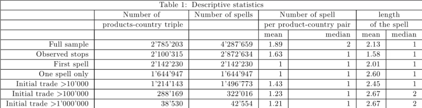
Table 1 presents summary statistics on duration of exports for our data. After correcting

for left censoring, the full sample data consists of 20₇₈₅0_{203 trade relationships}

(exporter-product-importer triplets) corresponding to 402870659 spells over the sample period

1996-2005. The average spell duration is only about two years and the median duration is one year, con…rming previous …ndings of Besedes and Prusa (2006). About one third of the spells are right censored. When considering single spell trade relationships the average duration increases. In a similar manner dropping all spells with initial trade value inferior to 10’000 dollars (100’000, or 1’000’000 dollars) increase the average and median duration. 65% of spells start with trade values lower to 10’000 dollars, 7,5% are initiated with trade values higher than 100’000 dollars and only 0,9% start with initial trade values greater than 1’000’000 dollars.

[Table 1: Descriptive Statistics]

Approximately 62% of trade relationships experience multiple spells. About 38% experience just two spells. Less than 20% have more than three spells (Table 2).

[Table 2: Description of exports duration data, 1996-2005]

4

Estimation results

4.1 Kaplan-Meier survival function

Before exploring the Cox estimations results, we begin characterizing duration of trade relationships non parametrically by estimating survival functions using the Kaplan-Meier estimator. In discrete time, the survivor function is de…ned as the probability that an individual survives at least to time t:

The Kaplan-Meier estimator of the survivor function at time t is de…ned as: ^

S(t) = ti t

[ni di=ni]

where ti, i = 1; 2::: is the ordered failure times, ni denotes the number of spells alive

(at risk) just before time ti, including those who will die at time ti. Let di denote the

number of failures (deaths) at time ti4.

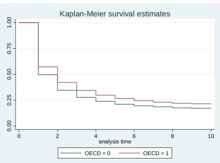
Figure 1 presents the Kaplan Meier estimator of the survival function for OECD and non OECD countries. Di¤erences in duration of exporting in the OECD and non OECD sample are important and signi…cant. In line with previous studies we observe that OECD exports survive signi…cantly longer than non OECD exports. The equality of the survival functions being rejected at a 1% level of signi…cance for all tests (Logrank, Cox, Wilcoxon, and Tarone Ware). Therefore in the remainder of the paper, we analyze separately OECD and non OECD samples’exports duration.

[Figure1: Kaplan Meier Survival Estimates]

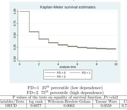
We identify industries according to their external …nance dependence (using Rajan and Zingales measure). We rank industries by increasing order. We then, estimate the survival function of the …rst and last quartile of the industries distribution. The

indus-try at the 25th percentile (low dependence) is beverages while the industry at the 75th

percentile (high dependence) is machinery. Duration of exports varies with the degree of external …nance dependence. Industries which are less dependent on external …nance have higher survival rate (Figure 2 and 3). This is to be expected as external …nance dependent sector are more vulnerable to liquidity shortages. This patterns is more ac-centuated for non OECD countries. We test for the equality of survival functions across industry types. The equality hypothesis is rejected for non OECD countries but we fail to reject it for OECD countries. Indeed, within the OECD sample, countries have similar level of …nancial development. Therefore, survival of …rms on the international market may not be limited by access to …nancial resources. While in the non OECD sample, variation in the level of …nancial development across countries allows for di¤erentiated survival of …rms based on their need for external …nance.

4_{The conditional probability that a spell dies in the time interval from t}

i to ti, given survival

up to time ti , is estimated as _ndi

i:The conditional probability that a spell survives beyond ti ,

given survival up to time ti , is estimated asni_ndi

i :In the limit as ! 0,

ni di

ni becomes an estimate

[Figure 2: Kaplan Meier Survival Estimates across di¤erent industries, non OECD sample]

[Figure 3:Kaplan Meier Survival Estimates across di¤erent industries, OECD sample]

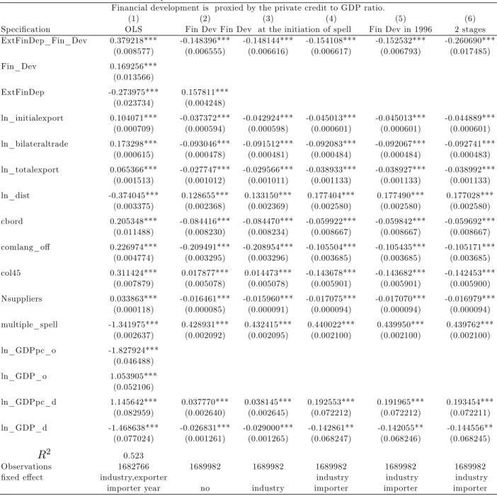
4.2 Baseline estimation

Table 3 details the estimation procedure to assess the e¤ect of …nancial development on duration of exports for non-OECD countries. In the …rst column we regress the length of trade relationships over a set of country and product speci…c covariates.

Lengthijkt0 = 0+ 1F in_Devjt0 Ext_F in_Deps+

X l 2

l:xlt0+ m+ "ijst0 (4)

where Lengthijkt0 is the duration of spell ijk initiated at t0. We include

exporter-time …xed e¤ects, importer and industry …xed e¤ects. We estimate equation (4) with conventional OLS. Results are reported in column (1). Although linear models are not appropriate for duration analysis, this gives us a …rst insight on the e¤ect of …nancial development on exports survival. The coe¢ cient on our intreaction term is positive and signi…cant; suggesting a positive e¤ect of …nancial development on the duration of exports.

Column (2) to (6) reports coe¢ cients obtained using a Cox semiparasitic propor-tional hazard model (equation(1)). We use exporter-time as the strati…cation variable. Column (2) reports results for the full sample (all trade relationships between 1996-2005) using the level of …nancial development at the initiation of the spell. In column (3) and (4) we report results adding consecutively industry and importer …xed e¤ects. In the following speci…cations we always control for industry and importer speci…c char-acteristics. Column (5) reports results using the level of …nancial development in 1996. Finally,we estimate equation (1) instrumenting the level of …nancial development by legal origin and the latitude of the exporting country, results are shown in columns (6). In column (4) to (6) since the speci…cation controls for exporting country-speci…c char-acteristics and industry-speci…c charchar-acteristics the interaction between external …nance dependence and …nancial development captures the e¤ect that varies both across coun-tries and induscoun-tries. Through out all speci…cations, the coe¢ cient on the interaction term remains negative and signi…cant. Financial development helps exports survival, by reducing the costs of external …nance to …rms which rely on external funds to support their operations.

Regarding traditional gravity covariates, all variables have expected sign and are highly signi…cant, suggesting that they successfully explain patterns and duration of trade. Distance as a proxy for trade costs increases exports hazard rate. A common border decreases the hazard rate , everything else held constant. Cultural proximity variables, colonial ties and sharing a common language both increase the likelihood of sustaining bilateral trade ‡ows over time.

The GDP of the importing country have expected negative sign. Interestingly, results suggests that holding GDP constant, exports to richer countries are on average shorter-lived. As changes in the level of GDPpc capture changing tastes and preferences in the importing country, GDPpc negatively in‡uences the probability of exports to survive over time.

Interestingly the hazard rate decreases with the number of competitors. A possible explanation for this …nding is as proposed by Nitsch (2007), that the number of com-petitors may just be a proxy for the size of the market. The multiple spells dummy variable increases the hazard rate. Suggesting as hypothesized by Besedes (2006), that multispell acts as an indicator of exporters poor reliability.

The initial export value plays a signi…cant role as implied by Rauch and Watson (2003). Duration increases with the transaction size, that is spell that start with higher initial value remain in existence for longer periods of time. The aggregate bilateral trade variable enters the regression negatively capturing the exporter’s knowledge of the import market. An increase in total exports of a product irrespective of the destination market favours duration, suggesting exporting experience is product speci…c.

[Table 3: Exports survival estimation results for nonOECD countries]

Results for OECD countries are shown in Table 4. Qualitatively results are similar for all speci…cations.

[Table 4: Exports survival estimation results for OECD countries]

4.3 Estimation for each cohort

We now estimate our baseline speci…cation for each cohort in the sample. we de…ne a cohort as the group of spells initiated the same year, we therefore have eight cohorts. Unlike in the baseline speci…cation, we are able to control for all dimensions including importer and industry …xed e¤ects. We use exporting country as the strati…cation variable. Results for non OECD (OECD) countries are reported in Table 5 (Table 6). Results for both non OECD and OECD countries are qualitatively similar to our baseline

results. The coe¢ cient on our main interaction term is negative and signi…cant but the e¤ect is three times smaller than in the baseline speci…cation (column (5) Tables 3 and 4). This is not surprising as we estimate our model for each cohort . This suggests that we may overestimate our coe¢ cients in our baseline speci…cation when considering full sample due to the fact we do not control for all …xed e¤ects dimensions.

[Table 5: Cox proportional hazard estimates, nonOECD countries] [Table 6: Cox proportional hazard estimates, OECD countries]

Table 7 and Table 8 show results where the level of …nancial development is instru-mented by legal origin and the latitude of the exporting country. Since we use estimated variable as a regressor we bootstrap standard errors. Results are qualitatively the same as in Table 5 and Table 6. All variables have expected sign and are all statistically signi…cant except for the interaction term coe¢ cient in the year 1997 for the OECD countries (column (2) Table 7) .

[Table 7: Cox proportional hazard estimates, non OECD countries Financial development instrumented]

[Table 8: Cox proportional hazard estimates, OECD countries Financial development instrumented]

5

Robustness checks

5.1 Using stock market capitalization

In order to test whether our results are driven by the choice of the …nancial development variable, we re-estimate all speci…cations using an alternative proxy for …nancial devel-opment, the ratio of stock market capitalization to GDP. Results are shown in Table (A) to (D).

Results are robust to the change in the …nancial development variable.

[Table A: Cox proportional hazard estimates, non OECD countries, using Stock market Capitalisation as a proxy for Financial development]

[Table B: Cox proportional hazard estimates, OECD countries, Financial development instrumented]

[Table C: Cox proportional hazard estimates, non OECD countries, using Stock market Capitalisation as a proxy for Financial development ]

[Table D: Cox proportional hazard estimates, OECD countries, Financial development instrumented]

6

Concluding Remarks

In this paper we examine empirically the duration of 121 developing countries’exports to OECD countries at the product level (6-digit level) from 1995 to 2005. We focus on the duration of trade relationships, that is the intensive margin of trade, using semi parametric model.

While …nancial development implication in …rms’ decision to export, has been es-tablished both theoretically and empirically (Melitz, 2003; Chaney 2005; Berman 2009), our purpose is to assess the distinct e¤ect of …nancial development on the duration of exports. Following seminal work of Rajan and Zingales we propose a distinctive method-ology to investigate a particular channel through which …nancial development may help exports survive longer, therefore, the causality is clearly identi…ed. By looking at the in-teraction term (between …nancial development and external …nance dependence) rather than the direct e¤ect of …nancial development and controlling for adequate country and industry …xed e¤ects, we reduce the number of variables that we rely on as well as possible omitted variable bias. Finally we control for possible endogeneity problem instrumenting the level of …nancial development following an two step procedure.

The main result of the paper is that …nancial development helps exports survival by reducing the costs of external …nance to …rms. Firms with facilitated access to external …nance can easily accommodate shocks and survive longer on the international market. This results is robust to a variety of robustness checks.

References

[1] References

[2] Álvarez, R. and López, R., 2008. Entry and exit in international markets: Evidence from Chilean

data. Review of International Economics

[3] Albornoz, F., H. Calvo Pardo and G. Corcos, “Sequential Exporting,” London School of Economics. Araujo, L. and E. Ornelas (2007), “Trust Based Trade,”CEP Discussion Paper 0820, London School of Economics.

[4] Alvarez, R. (2002), “Determinants of Firm Export Performance in a Less Developed Country,” mimeo, University of California at Los Angeles.

[5] Amurgo-Pacheco, A. and D. Pierola (2007), “Patterns of Export Diversi…cation in Developing Countries: Intensive and Extensive Margins,” mimeo, GIIS.

[6] Baldwin, R. and Harrigan, J. (2007), "Zeros, Quality, and Space: Trade Theory and Trade Evidence", NBER Working Paper Series 13214.

[7] Beck,Thorsten, Asli Demirgüç-Kunt and Ross Levine, 2000, "A New Database on Financial Development and Structure," World Bank Economic Review 14, pp. 597-605.

[8] Bekaert, Geert, Harvey, Campbell R. and Lundblad, Christian T.,Does Financial Liberalization Spur Growth?(September 2004). AFA 2002 Atlanta Meetings. [9] Bernard, A. and Jensen, B., 2004. Why some …rms export? Review of Economics

and Statistics, 86, 2.

[10] Bernard, A.; Redding, S.; and Schott, P., 2006. Multi-product …rms and product switching, NBER Working Paper 12293.

[11] Bernard, A. and Jensen, B., 2007. Firm structure, multinationals and manufactur-ing plant deaths.

Review of Economics and Statistics, 79, 2.

[12] Bernard, A., B. Jensen, S. Redding and P. Schott (2007), “Firms in International Trade,” NBER Working Paper Series 13054.

[13] Besedes, T. and Prusa T., 2006a,”Ins, Outs and the Duration of Trade,”Canadian Journal of Economics, 104, pp. 635-54.

[14] Besedes, T. and Prusa, T., 2006b. Production di¤erentiation and duration of U.S. import trade.

Journal of International Economics, 70, 2.

[15] Besedes, T. and Prusa, T., 2007. The role of extensive and intensive margins and export growth.

Paper prepared for INT-IDB, mimeo.

[16] Besedes, T. "A Search Cost Perspective on Duration of Trade," Departmental Working Papers 2006-12.

[17] Brenton P. & Newfarmer R. 2007. "Watching more than the Discovery channel to diversify export", in BREAKING INTO NEW MARKETS: Emerging Lessons for Export Diversi…cation, The World Bank.

[18] Brenton, P., Pierola M.D. and von Uexkull E. 2007. "The life and death of trade ‡ows understanding the survival rates of developing countries exporters "

[19] Brenton, P & Saborowski C. & von Uexkull E. 2009., "What explains the low survival rate of developing country export ‡ows ?," Policy Research Working Paper Series 4951, The World Bank

[20] Chaney, T. (2005). “Liquidity constrained exporters.”University of Chicago mimeo. [21] Cleves M, Goud W., Gutierrez R. An Introduction to Survival Analysis Using Stata,

StataPress.

[22] Do, Q.-T., Levchenko, A., 2007. "Comparative advantage, demand for external …nance, and …nancial development", Journal of Financial Economics 86, 796–834. [23] Gaulier, G. et al. (2008), "BACI: A World Database of International Trade Analysis

at the Product-level", CEPII Working Paper, 2008

[24] Manova K.,2008, Credit Constraints, "Equity Market Liberalizations and Interna-tional Trade", Journal of InternaInterna-tional Economics 76 p.33-47.

[25] Rajan, R., Zingales, L., 1998. Financial dependence and growth. American Eco-nomic Review 88, 559–586.

[26] Romalis, J., 2004. Factor proportions and the structure of commodity trade. Amer-ican Economic Review 94, 67–97.

[27] Svaleryd, H., Vlachos, J., 2005. Financial markets, the pattern of industrial spe-cialization and comparative advantage: evidence from OECD countries. European Economic Review 49, 113–144.

[28] Rauch, J., 1999, “Networks versus Markets in International Trade,” Journal of International Economics, 48, pp. 7-35. Rauch, J. (2007), “Development through Synergistic Reform,” NBER Working Paper Series 13170.

[29] Rauch, J. and Watson, J., 2003. Starting small in an unfamiliar environment. In-ternational Journal of Industrial Organization, 21.

[30] Roberts, M. and Tybout, J., 1997. An empirical model of sunk costs and the decision to export, American Economic Review, 87, 4.

[31] Volpe C and Carballo Jeronimo, 2008."Survival of New Exporters in Developing Countries:Does it Matter How They Diversify?", Int Working paper 04, IDB.

7

Figures and Tables

Figure1: Kaplan Meier Survival Estimates OECD vs nonOECD 0. 00 0. 25 0. 50 0. 75 1. 00 0 2 4 6 8 10 analysis time OECD = 0 OECD = 1

Kaplan-Meier survival estimates

Figure 2: Kaplan Meier Survival Estimates across di¤erent industries, non OECD sample

0. 00 0. 25 0. 50 0. 75 1. 00 0 2 4 6 8 10 analysis time FD = 0 FD = 1 FD = 2

Kaplan-Meier survival estimates

FD=1 25th percentile (low dependence)

FD=2 75th percentile (high dependence)

P values of the tests on equality of survival function ,Pr>chi2 Variables/Tests log rank Wilcoxon-Breslow-Gehan Tarone Ware Cox

Figure 3: Kaplan Meier Survival Estimates across di¤erent industries, OECD sample 0. 00 0. 25 0. 50 0. 75 1. 00 0 2 4 6 8 10 analysis time FD = 0 FD = 1 FD = 2

Kaplan-Meier survival estimates

FD=1 25th percentile (low dependence)

FD=2 75th percentile (high dependence)

P values of the tests on equality of survival function ,Pr>chi2 Variables/Tests log rank Wilcoxon-Breslow-Gehan Tarone Ware Cox

Table 1: Descriptive statistics

Number of Number of spells Number of spell length products-country triple per product-country pair of the spell

mean median mean median

Full sample 2’785’203 4’287’659 1.89 2 2.13 1

Observed stops 2’100’315 2’872’634 1.63 1 1.58 1

First spell 2’142’230 2’142’230 1 1 2.01 1

One spell only 1’644’947 1’644’947 1 1 2.60 1

Initial trade >10’000 1’214’143 1’496’773 1.43 1 2.45 1 Initial trade >100’000 288’169 322’016 1.23 1 2.67 2 Initial trade >1’000’000 38’530 42’554 1.21 1 2.67 2

Table 2: Description of exports duration data, 1996-2005 number of spells Freq. Percent Cum. 1 1,644,947 38.36 38.36 2 1,641,066 38.27 76.64 3 836,001 19.5 96.14 4 158,540 3.7 99.83 5 7,105 0.17 100 Total 4,287,659 100

Table 3: Exports survival estimation results for nonOECD countries Financial development is proxied by the private credit to GDP ratio.

(1) (2) (3) (4) (5) (6)

Speci…cation OLS Fin Dev Fin Dev at the initiation of spell Fin Dev in 1996 2 stages ExtFinDep_Fin_Dev 0.379218*** -0.148396*** -0.148144*** -0.154108*** -0.152532*** -0.260690*** (0.008577) (0.006555) (0.006616) (0.006617) (0.006793) (0.017485) Fin_Dev 0.169256*** (0.013566) ExtFinDep -0.273975*** 0.157811*** (0.023734) (0.004248) ln_initialexport 0.104071*** -0.037372*** -0.042924*** -0.045013*** -0.045013*** -0.044889*** (0.000709) (0.000594) (0.000598) (0.000601) (0.000601) (0.000601) ln_bilateraltrade 0.173298*** -0.093046*** -0.091512*** -0.092083*** -0.092067*** -0.092741*** (0.000615) (0.000478) (0.000481) (0.000484) (0.000484) (0.000483) ln_totalexport 0.065366*** -0.027747*** -0.029566*** -0.038933*** -0.038927*** -0.038992*** (0.001513) (0.001012) (0.001011) (0.001133) (0.001133) (0.001133) ln_dist -0.374045*** 0.128655*** 0.133150*** 0.177404*** 0.177490*** 0.177028*** (0.003375) (0.002368) (0.002369) (0.002580) (0.002580) (0.002580) cbord 0.205348*** -0.084416*** -0.084470*** -0.059922*** -0.059842*** -0.059692*** (0.011488) (0.008230) (0.008234) (0.008667) (0.008667) (0.008667) comlang_o¤ 0.226974*** -0.209491*** -0.208954*** -0.105504*** -0.105435*** -0.105171*** (0.004774) (0.003295) (0.003296) (0.003685) (0.003685) (0.003685) col45 0.311424*** 0.017877*** 0.014473*** -0.143678*** -0.143682*** -0.142453*** (0.007879) (0.005078) (0.005078) (0.005901) (0.005901) (0.005900) Nsuppliers 0.033863*** -0.016461*** -0.015960*** -0.017075*** -0.017070*** -0.016979*** (0.000118) (0.000085) (0.000091) (0.000094) (0.000094) (0.000094) multiple_spell -1.341975*** 0.428931*** 0.432415*** 0.440022*** 0.439950*** 0.439762*** (0.002637) (0.002092) (0.002095) (0.002100) (0.002100) (0.002100) ln_GDPpc_o -1.827924*** (0.046488) ln_GDP_o 1.053905*** (0.052106) ln_GDPpc_d 1.145642*** 0.037770*** 0.038145*** 0.192553*** 0.191965*** 0.193454*** (0.082959) (0.002640) (0.002645) (0.072212) (0.072212) (0.072211) ln_GDP_d -1.468638*** -0.026831*** -0.029000*** -0.142861** -0.142055** -0.144556** (0.077024) (0.001261) (0.001265) (0.068247) (0.068246) (0.068245) R2 0.523 Observations 1682766 1689982 1689982 1689982 1689982 1689982

…xed e¤ect industry,exporter industry industry industry

importer year no industry importer importer importer Standard errors in parentheses

T a b le 4 : E x p o rt s su rv iv a l e st im a ti o n re su lt s fo r n o n O E C D c o u n tr ie s F in a n c ia l d e v e lo p m e n t is p ro x ie d b y th e p ri v a te c re d it to G D P ra ti o . (1 ) (2 ) (3 ) (4 ) (5 ) (6 ) S p e c i… c a ti o n e O L S F in D e v F in D e v a t th e in it ia ti o n o f sp e ll F in D e v in 1 9 9 6 2 st a g e s E x tF in D e p * F in _ D e v 0 .1 5 3 4 9 4 8 * * * -0 .1 2 8 1 8 3 * * * -0 .1 1 1 6 3 5 * * * -0 .1 1 1 1 8 4 * * * -0 .1 6 0 4 4 2 * * * -0 .1 9 7 1 9 6 * * * 0 .0 0 6 7 3 3 (0 .0 0 5 7 6 0 ) (0 .0 0 5 8 0 1 ) (0 .0 0 5 8 0 5 ) (0 .0 0 5 6 7 8 ) (0 .0 0 8 2 7 8 ) F in _ D e v 0 .0 7 0 0 9 1 4 * * * 0 .0 0 6 1 0 2 7 E x tF in D e p 0 .2 6 7 2 1 2 9 * * * -0 .0 3 1 7 3 3 * * * 0 .0 2 3 1 2 0 9 (0 .0 0 5 1 2 0 ) ln _ in it ia le x p o rt 0 .1 1 1 5 9 7 9 * * * -0 .0 7 9 1 9 3 * * * -0 .0 8 2 5 3 4 * * * -0 .0 8 3 3 0 3 * * * -0 .0 8 3 2 1 0 * * * -0 .0 8 3 2 8 7 * * * 0 .0 0 0 5 4 9 4 (0 .0 0 0 4 8 7 ) (0 .0 0 0 4 9 1 ) (0 .0 0 0 4 9 1 ) (0 .0 0 0 4 9 1 ) (0 .0 0 0 4 9 1 ) ln _ b il a te ra lt ra d e .1 9 9 6 0 2 2 * * * -0 .1 0 4 0 1 8 * * * -0 .1 0 9 9 3 8 * * * -0 .1 1 0 9 9 3 * * * -0 .1 1 0 7 2 7 * * * -0 .1 1 0 7 4 5 * * * 0 0 0 5 8 3 2 (0 .0 0 0 4 4 0 ) (0 .0 0 0 4 4 8 ) (0 .0 0 0 4 5 1 ) (0 .0 0 0 4 5 1 ) (0 .0 0 0 4 5 2 ) ln _ to ta le x p o rt 0 .3 4 9 1 2 0 6 * * * -0 .1 7 7 6 1 2 * * * -0 .1 7 9 3 3 0 * * * -0 .1 7 8 8 3 7 * * * -0 .1 7 8 7 9 1 * * * -0 .1 7 8 2 8 0 * * * 0 .0 0 1 7 8 7 (0 .0 0 1 2 3 7 ) (0 .0 0 1 2 3 8 ) (0 .0 0 1 4 3 4 ) (0 .0 0 1 4 3 4 ) (0 .0 0 1 4 3 4 ) ln _ d is t -0 .1 9 3 4 6 8 4 * * * 0 .0 2 5 2 5 1 * * * 0 .0 2 9 3 4 2 * * * 0 .1 4 3 3 8 5 * * * 0 .1 4 3 5 1 2 * * * 0 .1 4 3 2 7 4 * * * 0 .0 0 2 6 5 0 8 (0 .0 0 1 4 1 3 ) (0 .0 0 1 4 1 3 ) (0 .0 0 2 2 2 6 ) (0 .0 0 2 2 2 5 ) (0 .0 0 2 2 2 6 ) c b o rd 0 .1 6 5 5 4 4 8 * * * -0 .3 3 0 4 2 3 * * * -0 .3 2 9 2 8 8 * * * -0 .2 1 3 9 6 8 * * * -0 .2 1 4 0 1 5 * * * -0 .2 1 5 8 4 5 * * * 0 .0 0 4 8 1 2 (0 .0 0 4 0 8 7 ) (0 .0 0 4 0 8 7 ) (0 .0 0 4 3 0 8 ) (0 .0 0 4 3 0 8 ) (0 .0 0 4 3 0 8 ) c o m la n g _ o ¤ 0 .1 9 1 1 6 7 * * * -0 .1 9 8 5 1 4 * * * -0 .1 9 8 1 5 4 * * * -0 .1 4 7 9 1 2 * * * -0 .1 4 8 1 2 1 * * * -0 .1 4 6 8 6 2 * * * 0 .0 0 4 4 4 8 2 (0 .0 0 3 5 3 1 ) (0 .0 0 3 5 3 1 ) (0 .0 0 3 7 5 8 ) (0 .0 0 3 7 5 8 ) (0 .0 0 3 7 5 8 ) c o l4 5 0 .2 6 4 1 3 4 5 * * * -0 .5 6 1 6 8 6 * * * -0 .5 4 5 9 3 1 * * * -0 .2 0 1 2 3 0 * * * -0 .2 0 3 1 2 6 * * * -0 .2 0 8 6 6 7 * * * 0 .0 0 4 4 4 8 2 (0 .0 1 8 2 3 4 ) (0 .0 1 8 2 3 7 ) (0 .0 1 9 1 2 3 ) (0 .0 1 9 1 2 2 ) (0 .0 1 9 1 2 8 ) N su p p li e rs 0 .0 5 0 0 3 6 6 * * * -0 .0 3 7 2 5 8 * * * -0 .0 3 4 3 5 3 * * * -0 .0 3 6 1 0 4 * * * -0 .0 3 6 2 0 4 * * * -0 .0 3 6 1 6 5 * * * 0 .0 0 0 1 2 6 5 (0 .0 0 0 1 0 4 ) (0 .0 0 0 1 1 2 ) (0 .0 0 0 1 1 5 ) (0 .0 0 0 1 1 5 ) (0 .0 0 0 1 1 5 ) m u lt ip le _ sp e ll -2 .1 7 8 3 1 9 * * * 0 .9 8 0 2 2 1 * * * 0 .9 8 5 8 6 7 * * * 0 .9 8 7 8 5 2 * * * 0 .9 8 7 6 2 0 * * * 0 .9 8 7 6 1 7 * * * 0 .0 0 2 2 1 9 7 (0 .0 0 2 0 3 9 ) (0 .0 0 2 0 4 1 ) (0 .0 0 2 0 4 0 ) (0 .0 0 2 0 4 0 ) (0 .0 0 2 0 4 0 ) ln _ G D P p c _ d -2 .1 2 8 0 6 2 * * * 0 .1 3 2 4 7 7 * * * 0 .1 2 2 6 5 8 * * * 0 .0 3 4 9 4 6 0 .0 3 6 9 1 7 0 .0 3 7 0 5 4 0 .0 0 2 2 1 9 7 (0 .0 0 2 1 2 8 ) (0 .0 0 2 1 3 2 ) (0 .0 5 6 6 4 5 ) (0 .0 5 6 6 4 4 ) (0 .0 5 6 6 4 4 ) ln _ G D P _ d 2 .8 5 8 5 2 5 * * * 0 .1 4 0 6 7 6 * * * 0 .1 3 2 6 6 4 * * * 0 .3 7 8 4 6 1 * * * 0 .3 7 5 8 6 7 * * * 0 .3 7 5 6 2 3 * * * 0 .0 5 8 2 5 0 6 (0 .0 0 1 1 9 0 ) (0 .0 0 1 1 9 6 ) (0 .0 5 4 7 5 1 ) (0 .0 5 4 7 5 1 ) (0 .0 5 4 7 5 1 ) ln _ G D P p c _ o -0 .8 0 6 1 9 9 8 * * * 5 9 7 8 4 2 ln _ G D P _ o -0 .3 5 6 0 6 6 1 * * * 0 .0 5 6 6 7 6 8 R 2 0 .7 2 . . . . . . O b se rv a ti o n s 2 9 0 4 2 8 2 2 9 0 4 2 8 2 2 9 0 4 2 8 2 2 9 0 4 2 8 2 2 9 0 4 2 8 2 2 9 0 4 2 8 2 F ix e d e ¤ e c t n o fe . in d u st ry ,i m p o rt e r. .i n d u st ry ,i m p o rt e r in d u st ry ,i m p o rt e r. in d u st ry ,i m p o rt e r. in d u st ry ,i m p o rt e r. S ta n d a rd e rr o rs in p a re n th e se s * * * p < 0 .0 1 , * * p < 0 .0 5 , * p < 0 .1

T a b le 5 : C o x p ro p o rt io n a l h a z a rd e st im a te s, n o n O E C D c o u n tr ie s O u r m e a su re o f … n a n c ia l d e v e lo p m e n t is th e p ri v a te c re d it to G D P ra ti o . (1 ) (2 ) (3 ) (4 ) (5 ) (6 ) (7 ) (8 ) (9 ) Y e a r 1 9 9 6 1 9 9 7 1 9 9 8 1 9 9 9 2 0 0 0 2 0 0 1 2 0 0 2 2 0 0 3 2 0 0 4 E x t_ F in _ D e p * F in _ D e v -0 .0 9 1 6 8 0 * * * -0 .0 9 5 9 1 6 * * * -0 .0 8 7 9 2 3 * * * -0 .1 8 6 1 1 7 * * * -0 .1 4 5 1 4 4 * * * -0 .1 1 9 1 7 0 * * * -0 .1 5 7 7 3 8 * * * -0 .1 4 3 7 0 0 * * * -0 .0 8 7 1 6 0 * * * (0 .0 1 5 3 0 4 ) (0 .0 1 8 3 9 4 ) (0 .0 1 6 6 8 2 ) (0 .0 1 8 3 4 4 ) (0 .0 2 0 6 6 3 ) (0 .0 2 1 4 8 4 ) (0 .0 2 2 4 0 9 ) (0 .0 2 4 7 3 6 ) (0 .0 2 9 1 9 7 ) lo g in it ia l_ e x p o rt -0 .0 8 1 2 9 0 * * * -0 .0 1 9 7 8 0 * * * -0 .0 1 7 7 4 9 * * * -0 .0 2 2 6 9 9 * * * -0 .0 2 6 0 3 3 * * * -0 .0 2 7 8 1 5 * * * -0 .0 3 3 4 0 8 * * * -0 .0 3 1 1 5 6 * * * -0 .0 2 5 0 2 3 * * * (0 .0 0 1 5 3 4 ) (0 .0 0 1 9 2 7 ) (0 .0 0 1 9 4 2 ) (0 .0 0 1 9 1 3 ) (0 .0 0 1 7 0 9 ) (0 .0 0 1 7 5 7 ) (0 .0 0 1 7 7 4 ) (0 .0 0 1 7 2 2 ) (0 .0 0 1 8 6 6 ) lo g d is t 0 .2 2 6 9 5 2 * * * 0 .1 5 7 9 3 8 * * * 0 .1 5 5 7 9 7 * * * 0 .1 5 0 6 7 3 * * * 0 .1 4 5 0 5 8 * * * 0 .1 3 0 9 1 6 * * * 0 .1 1 4 5 4 5 * * * 0 .1 2 9 6 3 6 * * * 0 .1 1 7 4 2 1 * * * (0 .0 0 6 6 9 2 ) (0 .0 0 7 6 2 4 ) (0 .0 0 7 8 2 9 ) (0 .0 0 7 5 4 0 ) (0 .0 0 7 3 7 3 ) (0 .0 0 7 5 0 0 ) (0 .0 0 7 4 8 9 ) (0 .0 0 7 7 6 7 ) (0 .0 0 8 6 6 6 ) c b o rd -0 .1 3 4 5 0 7 * * * -0 .0 9 6 8 8 5 * * * -0 .0 9 0 0 3 4 * * * -0 .0 6 2 2 0 7 * * * -0 .0 3 0 6 1 7 -0 .0 5 6 4 7 8 * * -0 .0 5 4 4 7 8 * * -0 .0 6 8 2 5 5 * * 0 .0 2 3 7 8 6 (0 .0 2 0 1 5 0 ) (0 .0 2 3 5 6 7 ) (0 .0 2 4 1 7 5 ) (0 .0 2 3 9 2 1 ) (0 .0 2 3 4 7 0 ) (0 .0 2 4 6 9 7 ) (0 .0 2 5 9 1 4 ) (0 .0 2 6 7 9 8 ) (0 .0 2 9 2 6 6 ) c o m la n g _ o ¤ -0 .1 3 5 9 0 3 * * * -0 .0 7 8 8 8 4 * * * -0 .0 7 4 1 6 7 * * * -0 .0 8 5 6 6 8 * * * -0 .0 8 3 4 8 7 * * * -0 .0 9 3 3 5 0 * * * -0 .1 0 5 6 8 4 * * * -0 .0 8 2 0 8 1 * * * -0 .0 7 2 1 2 4 * * * (0 .0 0 9 3 8 1 ) (0 .0 1 1 1 1 6 ) (0 .0 1 1 3 0 5 ) (0 .0 1 0 9 5 9 ) (0 .0 1 0 7 5 4 ) (0 .0 1 1 1 2 5 ) (0 .0 1 1 0 3 9 ) (0 .0 1 1 3 6 5 ) (0 .0 1 2 9 0 7 ) c o l -0 .2 1 0 3 3 6 * * * -0 .1 2 3 6 4 1 * * * -0 .0 9 4 8 5 1 * * * -0 .1 1 4 2 1 2 * * * -0 .1 1 7 6 9 3 * * * -0 .1 1 2 8 2 0 * * * -0 .0 7 4 9 3 7 * * * -0 .0 7 5 7 1 2 * * * -0 .0 4 8 0 7 2 * * (0 .0 1 4 6 5 0 ) (0 .0 1 7 8 3 3 ) (0 .0 1 7 4 4 5 ) (0 .0 1 7 1 9 8 ) (0 .0 1 7 1 5 6 ) (0 .0 1 7 3 9 8 ) (0 .0 1 7 4 4 5 ) (0 .0 1 8 8 1 2 ) (0 .0 2 0 9 0 8 ) lo g b il a te ra l_ tr a d e -0 .1 2 5 1 7 4 * * * -0 .0 9 0 3 4 3 * * * -0 .0 8 8 0 4 0 * * * -0 .0 8 7 5 9 0 * * * -0 .0 7 7 7 7 6 * * * -0 .0 7 1 5 0 8 * * * -0 .0 7 1 8 7 0 * * * -0 .0 6 5 1 4 4 * * * -0 .0 5 3 9 1 9 * * * (0 .0 0 1 2 8 6 ) (0 .0 0 1 4 6 9 ) (0 .0 0 1 4 8 7 ) (0 .0 0 1 4 5 4 ) (0 .0 0 1 3 8 2 ) (0 .0 0 1 4 1 0 ) (0 .0 0 1 4 2 5 ) (0 .0 0 1 4 1 8 ) (0 .0 0 1 5 4 2 ) lo g to ta l_ e x p o rt -0 .0 6 8 9 3 8 * * * -0 .0 4 5 7 0 3 * * * -0 .0 4 5 5 2 1 * * * -0 .0 4 2 8 7 6 * * * -0 .0 3 2 1 0 7 * * * -0 .0 2 8 0 2 5 * * * -0 .0 3 4 1 9 9 * * * -0 .0 2 0 6 8 9 * * * -0 .0 1 7 1 3 5 * * * (0 .0 0 3 0 9 0 ) (0 .0 0 3 5 7 2 ) (0 .0 0 3 6 2 0 ) (0 .0 0 3 4 5 9 ) (0 .0 0 3 2 4 2 ) (0 .0 0 3 2 5 0 ) (0 .0 0 3 2 8 3 ) (0 .0 0 3 2 8 2 ) (0 .0 0 3 5 6 6 ) N _ su p p li e rs -0 .0 2 5 6 5 2 * * * -0 .0 1 5 3 8 6 * * * -0 .0 1 4 6 0 3 * * * -0 .0 1 3 9 4 3 * * * -0 .0 1 3 5 1 7 * * * -0 .0 1 2 1 8 2 * * * -0 .0 1 2 4 7 5 * * * -0 .0 1 1 3 7 4 * * * -0 .0 1 1 5 5 6 * * * (0 .0 0 0 2 4 5 ) (0 .0 0 0 2 9 4 ) (0 .0 0 0 2 9 1 ) (0 .0 0 0 2 8 2 ) (0 .0 0 0 2 7 2 ) (0 .0 0 0 2 7 4 ) (0 .0 0 0 2 7 6 ) (0 .0 0 0 2 7 7 ) (0 .0 0 0 3 0 7 ) m u lt ip le _ sp e ll 1 .5 4 2 4 5 1 * * * 0 .6 7 8 8 8 9 * * * 0 .4 1 3 6 6 0 * * * 0 .2 8 4 1 2 8 * * * 0 .2 0 5 9 4 9 * * * 0 .1 1 8 6 1 4 * * * 0 .0 5 0 6 9 0 * * * -0 .0 3 4 7 2 2 * * * -0 .2 3 3 4 2 9 * * * (0 .0 0 5 9 8 0 ) (0 .0 0 6 4 0 4 ) (0 .0 0 6 3 6 2 ) (0 .0 0 6 2 4 3 ) (0 .0 0 6 1 3 6 ) (0 .0 0 6 2 3 2 ) (0 .0 0 6 2 1 1 ) (0 .0 0 6 2 9 7 ) (0 .0 0 7 2 1 1 ) O b se rv a ti o n s 2 8 6 2 8 7 1 4 0 4 6 0 1 4 1 4 3 5 1 5 1 9 5 7 1 5 7 7 2 2 1 5 4 2 2 3 1 6 2 9 8 0 1 7 2 8 8 2 1 8 0 6 9 8 S ta n d a rd e rr o rs in p a re n th e se s * * * p < 0 .0 1 , * * p < 0 .0 5 , * p < 0 .1

T a b le 6 : C o x p ro p o rt io n a l h a z a rd e st im a te s, O E C D c o u n tr ie s O u r m e a su re o f … n a n c ia l d e v e lo p m e n t is th e p ri v a te c re d it to G D P ra ti o . (1 ) (2 ) (3 ) (4 ) (5 ) (6 ) (7 ) (8 ) (9 ) Y e a r 1 9 9 6 1 9 9 7 1 9 9 8 1 9 9 9 2 0 0 0 2 0 0 1 2 0 0 2 2 0 0 3 2 0 0 4 E x t_ F in _ D e p * F in _ D e v _ h a t -0 .0 5 5 3 9 7 * * -0 .0 3 6 1 9 5 -0 .0 7 1 1 1 4 * * * -0 .0 8 8 4 8 4 * * * -0 .0 8 1 1 4 2 * * * -0 .0 6 4 2 8 0 * * -0 .0 6 6 8 4 9 * * -0 .0 4 7 2 1 5 -0 .0 8 8 9 9 1 * * * (0 .0 2 4 0 7 4 ) (0 .0 2 4 0 0 2 ) (0 .0 2 4 3 9 8 ) (0 .0 2 4 9 0 1 ) (0 .0 2 5 2 6 0 ) (0 .0 2 6 3 1 8 ) (0 .0 2 7 0 5 6 ) (0 .0 2 8 8 4 4 ) (0 .0 3 3 9 2 3 ) lo g in it ia l_ e x p o rt -0 .0 2 8 8 9 5 * * * -0 .0 2 9 2 3 4 * * * -0 .0 3 0 7 6 1 * * * -0 .0 3 7 3 7 3 * * * -0 .0 3 5 7 8 6 * * * -0 .0 3 9 2 1 0 * * * -0 .0 4 3 4 9 8 * * * -0 .0 4 1 5 6 3 * * * -0 .0 3 9 4 0 8 * * * (0 .0 0 1 4 5 1 ) (0 .0 0 1 4 5 6 ) (0 .0 0 1 5 0 9 ) (0 .0 0 1 5 3 5 ) (0 .0 0 1 4 8 6 ) (0 .0 0 1 5 7 0 ) (0 .0 0 1 5 8 8 ) (0 .0 0 1 6 1 0 ) (0 .0 0 1 8 3 3 ) lo g d is t 0 .0 7 9 0 6 8 * * * 0 .0 8 4 0 1 2 * * * 0 .0 9 5 7 2 1 * * * 0 .0 8 9 5 5 8 * * * 0 .0 9 7 7 8 4 * * * 0 .0 9 8 4 4 4 * * * 0 .1 0 8 1 4 4 * * * 0 .0 9 6 6 0 5 * * * 0 .1 2 2 5 5 4 * * * (0 .0 0 6 4 4 8 ) (0 .0 0 6 4 3 3 ) (0 .0 0 6 6 5 8 ) (0 .0 0 6 6 7 7 ) (0 .0 0 6 8 0 6 ) (0 .0 0 7 1 2 9 ) (0 .0 0 7 2 2 5 ) (0 .0 0 7 8 0 6 ) (0 .0 0 9 2 5 9 ) c b o rd -0 .1 0 3 7 3 7 * * * -0 .0 8 4 1 7 9 * * * -0 .0 7 7 5 3 3 * * * -0 .1 2 0 0 0 9 * * * -0 .1 0 1 4 7 1 * * * -0 .1 1 5 3 9 0 * * * -0 .1 3 7 6 4 5 * * * -0 .1 8 0 9 0 2 * * * -0 .1 9 1 3 7 4 * * * (0 .0 1 2 1 7 6 ) (0 .0 1 2 2 9 0 ) (0 .0 1 2 7 6 8 ) (0 .0 1 2 8 4 2 ) (0 .0 1 3 1 4 8 ) (0 .0 1 3 6 5 8 ) (0 .0 1 4 3 5 7 ) (0 .0 1 5 6 0 1 ) (0 .0 1 8 3 3 4 ) c o m la n g _ o ¤ -0 .0 9 9 9 0 4 * * * -0 .1 1 1 9 1 3 * * * -0 .0 9 9 3 2 9 * * * -0 .0 9 9 0 2 7 * * * -0 .1 1 3 9 5 6 * * * -0 .1 0 2 7 7 4 * * * -0 .0 8 9 4 3 8 * * * -0 .0 7 0 4 8 6 * * * -0 .1 0 4 4 2 1 * * * (0 .0 1 0 5 9 0 ) (0 .0 1 0 7 3 7 ) (0 .0 1 0 9 8 4 ) (0 .0 1 1 1 3 8 ) (0 .0 1 1 3 4 7 ) (0 .0 1 1 8 3 8 ) (0 .0 1 1 9 2 9 ) (0 .0 1 3 2 9 9 ) (0 .0 1 6 0 0 5 ) c o l -0 .1 0 5 3 7 3 * -0 .1 5 3 7 5 8 * * * -0 .2 0 3 5 4 0 * * * -0 .2 3 4 4 4 8 * * * -0 .1 4 5 6 1 9 * * -0 .1 2 1 1 4 2 * -0 .1 5 7 1 2 1 * * -0 .1 0 4 3 3 5 -0 .2 2 5 6 6 1 * * (0 .0 5 6 1 9 6 ) (0 .0 5 6 9 2 5 ) (0 .0 6 2 1 7 0 ) (0 .0 5 3 8 4 3 ) (0 .0 5 8 6 3 7 ) (0 .0 6 3 4 6 3 ) (0 .0 6 8 1 3 7 ) (0 .0 7 2 4 9 2 ) (0 .0 9 1 5 8 8 ) lo g b il a te ra l_ tr a d e -0 .0 9 8 0 3 6 * * * -0 .0 9 0 6 2 0 * * * -0 .0 9 3 0 3 0 * * * -0 .0 9 0 4 6 3 * * * -0 .0 8 6 1 3 0 * * * -0 .0 8 4 9 8 4 * * * -0 .0 8 3 5 3 6 * * * -0 .0 7 6 7 5 4 * * * -0 .0 6 5 7 4 7 * * * (0 .0 0 1 3 2 5 ) (0 .0 0 1 3 1 1 ) (0 .0 0 1 3 4 5 ) (0 .0 0 1 3 4 9 ) (0 .0 0 1 3 4 8 ) (0 .0 0 1 3 9 8 ) (0 .0 0 1 4 1 6 ) (0 .0 0 1 4 7 7 ) (0 .0 0 1 6 9 8 ) lo g to ta l_ e x p o rt -0 .1 6 0 2 7 5 * * * -0 .1 5 0 2 7 5 * * * -0 .1 4 3 7 8 4 * * * -0 .1 3 6 8 3 8 * * * -0 .1 2 7 7 4 4 * * * -0 .1 3 2 3 0 3 * * * -0 .1 2 0 7 5 8 * * * -0 .1 1 9 8 3 8 * * * -0 .0 8 9 8 5 1 * * * (0 .0 0 4 2 0 9 ) (0 .0 0 4 2 7 7 ) (0 .0 0 4 4 6 1 ) (0 .0 0 4 3 9 4 ) (0 .0 0 4 4 0 9 ) (0 .0 0 4 6 5 7 ) (0 .0 0 4 6 8 8 ) (0 .0 0 5 1 3 0 ) (0 .0 0 5 8 6 9 ) N _ su p p li e rs -0 .0 2 6 3 8 6 * * * -0 .0 2 5 3 3 0 * * * -0 .0 2 4 7 9 4 * * * -0 .0 2 5 6 6 2 * * * -0 .0 2 4 8 8 7 * * * -0 .0 2 5 3 2 6 * * * -0 .0 2 5 0 4 3 * * * -0 .0 2 4 8 9 9 * * * -0 .0 2 7 0 0 8 * * * (0 .0 0 0 3 5 9 ) (0 .0 0 0 3 5 2 ) (0 .0 0 0 3 5 6 ) (0 .0 0 0 3 5 2 ) (0 .0 0 0 3 5 0 ) (0 .0 0 0 3 6 4 ) (0 .0 0 0 3 6 6 ) (0 .0 0 0 3 8 5 ) (0 .0 0 0 4 4 6 ) m u lt ip le _ sp e ll 1 .2 1 5 7 0 6 * * * 1 .1 2 6 2 9 3 * * * 0 .8 6 0 3 7 7 * * * 0 .6 8 6 3 3 7 * * * 0 .5 3 3 2 9 7 * * * 0 .4 1 8 7 6 6 * * * 0 .3 1 1 9 4 2 * * * 0 .1 5 3 0 8 5 * * * -0 .1 1 7 0 0 7 * * * (0 .0 0 6 1 2 7 ) (0 .0 0 5 8 3 5 ) (0 .0 0 5 6 7 1 ) (0 .0 0 5 5 8 0 ) (0 .0 0 5 5 8 6 ) (0 .0 0 5 7 2 7 ) (0 .0 0 5 7 3 8 ) (0 .0 0 5 9 4 8 ) (0 .0 0 6 7 7 8 ) O b se rv a ti o n s 2 2 7 6 1 5 2 2 6 8 5 6 2 1 4 6 2 2 2 1 7 7 2 8 2 1 6 9 8 6 2 0 8 9 9 3 2 2 0 9 2 6 2 1 9 1 2 8 2 3 6 5 8 5 S ta n d a rd e rr o rs in p a re n th e se s * * * p < 0 .0 1 , * * p < 0 .0 5 , * p < 0 .1

T a b le 7 : C o x p ro p o rt io n a l h a z a rd e st im a te s, n o n O E C D c o u n tr ie s O u r m e a su re o f … n a n c ia l d e v e lo p m e n t is th e p ri v a te c re d it to G D P ra ti o , in st ru m e n te d . (1 ) (2 ) (3 ) (4 ) (5 ) (6 ) (7 ) (8 ) Y e a r 1 9 9 6 1 9 9 7 1 9 9 8 1 9 9 9 2 0 0 0 2 0 0 1 2 0 0 2 2 0 0 3 E x t_ F in _ D e p * F in _ D e v _ h a t -0 .0 5 6 1 9 3 * -0 .1 1 6 8 3 5 * * * -0 .1 6 5 7 9 7 * * * -0 .1 0 7 0 7 7 * * * -0 .1 5 3 6 0 9 * * * -0 .1 6 8 4 6 3 * * * -0 .0 9 9 7 2 4 * * * -0 .0 6 6 7 7 6 * (0 .0 3 2 7 3 0 ) (0 .0 3 0 1 1 1 ) (0 .0 3 3 9 9 7 ) (0 .0 3 3 3 5 8 ) (0 .0 2 8 3 9 1 ) (0 .0 3 5 4 7 8 ) (0 .0 2 8 4 8 2 ) (0 .0 3 4 1 9 6 ) lo g in it ia l_ e x p o rt -0 .0 2 1 2 3 4 * * * -0 .0 1 4 7 5 3 * * * -0 .0 1 9 8 9 4 * * * -0 .0 2 4 4 0 6 * * * -0 .0 2 6 5 1 2 * * * -0 .0 3 1 8 7 1 * * * -0 .0 3 1 3 2 8 * * * -0 .0 2 5 6 4 1 * * * (0 .0 0 1 1 7 1 ) (0 .0 0 1 1 7 4 ) (0 .0 0 1 1 9 1 ) (0 .0 0 1 0 0 8 ) (0 .0 0 1 3 5 7 ) (0 .0 0 1 1 7 7 ) (0 .0 0 1 1 3 4 ) (0 .0 0 1 3 1 2 ) lo g d is t 0 .1 5 3 7 3 4 * * * 0 .1 5 5 3 7 5 * * * 0 .1 5 3 3 8 1 * * * 0 .1 4 7 2 6 8 * * * 0 .1 3 0 9 4 1 * * * 0 .1 1 4 2 3 6 * * * 0 .1 3 4 2 6 1 * * * 0 .1 1 5 1 4 1 * * * (0 .0 0 4 7 8 8 ) (0 .0 0 5 2 4 9 ) (0 .0 0 4 6 9 5 ) (0 .0 0 4 5 9 7 ) (0 .0 0 5 3 3 4 ) (0 .0 0 4 1 6 9 ) (0 .0 0 4 8 0 9 ) (0 .0 0 5 2 3 4 ) c b o rd -0 .1 2 1 6 0 0 * * * -0 .0 8 0 7 3 7 * * * -0 .0 5 7 0 7 7 * * * -0 .0 2 0 9 2 0 -0 .0 5 3 0 1 4 * * * -0 .0 3 7 5 7 6 * * -0 .0 5 6 2 8 4 * * * 0 .0 1 2 9 6 0 (0 .0 1 4 9 5 3 ) (0 .0 1 6 3 1 2 ) (0 .0 1 5 3 2 5 ) (0 .0 1 8 2 0 9 ) (0 .0 1 2 5 3 6 ) (0 .0 1 7 2 7 5 ) (0 .0 1 7 9 3 2 ) (0 .0 1 7 7 0 9 ) c o m la n g _ o ¤ -0 .0 8 2 8 2 7 * * * -0 .0 7 2 0 0 0 * * * -0 .0 7 9 8 5 0 * * * -0 .0 7 8 8 2 6 * * * -0 .0 8 9 9 9 2 * * * -0 .0 9 6 8 2 6 * * * -0 .0 8 0 7 0 4 * * * -0 .0 6 1 0 7 7 * * * (0 .0 0 7 9 8 9 ) (0 .0 0 7 6 8 2 ) (0 .0 0 5 8 3 8 ) (0 .0 0 6 6 5 0 ) (0 .0 0 7 2 6 8 ) (0 .0 0 5 6 9 1 ) (0 .0 0 7 1 5 1 ) (0 .0 0 8 5 5 6 ) c o l -0 .1 3 5 2 9 6 * * * -0 .0 9 6 5 8 1 * * * -0 .1 1 8 0 2 6 * * * -0 .1 2 9 1 1 3 * * * -0 .1 2 4 9 4 8 * * * -0 .0 8 5 4 0 7 * * * -0 .0 8 0 4 9 4 * * * -0 .0 5 7 3 5 5 * * * (0 .0 1 1 8 2 6 ) (0 .0 1 2 2 7 3 ) (0 .0 0 9 3 9 8 ) (0 .0 0 9 8 6 5 ) (0 .0 1 0 4 4 8 ) (0 .0 1 0 0 3 8 ) (0 .0 1 0 7 7 5 ) (0 .0 1 0 8 3 2 ) lo g b il a te ra l_ tr a d e -0 .0 9 3 9 4 2 * * * -0 .0 9 0 1 4 6 * * * -0 .0 9 1 2 0 4 * * * -0 .0 8 0 8 5 5 * * * -0 .0 7 4 7 8 4 * * * -0 .0 7 4 4 5 7 * * * -0 .0 6 7 3 2 2 * * * -0 .0 5 5 5 7 4 * * * (0 .0 0 1 0 4 9 ) (0 .0 0 0 9 7 3 ) (0 .0 0 0 8 4 9 ) (0 .0 0 0 7 8 0 ) (0 .0 0 0 9 9 3 ) (0 .0 0 1 0 6 4 ) (0 .0 0 0 8 2 4 ) (0 .0 0 0 9 6 4 ) lo g to ta l_ e x p o rt -0 .0 4 8 0 5 4 * * * -0 .0 4 9 3 2 5 * * * -0 .0 4 5 7 2 5 * * * -0 .0 3 4 5 6 7 * * * -0 .0 2 9 7 4 9 * * * -0 .0 3 5 2 7 9 * * * -0 .0 1 8 5 9 3 * * * -0 .0 1 7 0 4 4 * * * (0 .0 0 1 8 9 3 ) (0 .0 0 1 9 6 1 ) (0 .0 0 2 1 2 7 ) (0 .0 0 1 5 6 4 ) (0 .0 0 1 8 1 4 ) (0 .0 0 1 9 7 8 ) (0 .0 0 1 5 8 3 ) (0 .0 0 1 8 0 0 ) N _ su p p li e rs -0 .0 1 6 5 4 4 * * * -0 .0 1 4 9 8 9 * * * -0 .0 1 4 4 1 8 * * * -0 .0 1 3 8 9 8 * * * -0 .0 1 2 5 7 5 * * * -0 .0 1 2 5 2 6 * * * -0 .0 1 1 5 9 1 * * * -0 .0 1 1 2 1 7 * * * (0 .0 0 0 1 7 8 ) (0 .0 0 0 1 8 9 ) (0 .0 0 0 1 8 5 ) (0 .0 0 0 1 8 1 ) (0 .0 0 0 1 4 9 ) (0 .0 0 0 1 8 0 ) (0 .0 0 0 1 8 7 ) (0 .0 0 0 2 0 6 ) m u lt ip le _ sp e ll 0 .7 6 4 1 4 3 * * * 0 .5 6 5 4 8 3 * * * 0 .4 4 3 6 1 5 * * * 0 .3 2 6 5 9 1 * * * 0 .2 0 8 9 0 7 * * * 0 .1 1 9 2 8 5 * * * 0 .0 0 8 9 4 1 * * -0 .2 0 6 2 0 0 * * * (0 .0 0 3 6 8 5 ) (0 .0 0 3 3 1 6 ) (0 .0 0 3 2 4 0 ) (0 .0 0 3 2 1 9 ) (0 .0 0 4 0 7 2 ) (0 .0 0 3 8 3 4 ) (0 .0 0 3 5 2 3 ) (0 .0 0 4 6 0 2 ) O b se rv a ti o n s 1 5 8 0 2 9 1 5 9 0 9 3 1 7 0 2 7 6 1 7 6 4 9 6 1 7 3 1 7 5 1 8 4 2 4 3 1 9 6 8 1 6 2 0 6 0 9 8 B o o ts tr a p p e d S ta n d a rd e rr o rs in p a re n th e se s * * * p < 0 .0 1 , * * p < 0 .0 5 , * p < 0 .1

T a b le 8 : C o x p ro p o rt io n a l h a z a rd e st im a te s, O E C D c o u n tr ie s O u r m e a su re o f … n a n c ia l d e v e lo p m e n t is th e p ri v a te c re d it to G D P ra ti o , in st ru m e n te d . (1 ) (2 ) (3 ) (4 ) (5 ) (6 ) (7 ) (8 ) (9 ) Y e a r 1 9 9 6 1 9 9 7 1 9 9 8 1 9 9 9 2 0 0 0 2 0 0 1 2 0 0 2 2 0 0 3 2 0 0 4 E x t_ F in _ D e p * F in _ D e v _ h a t -0 .0 5 5 3 9 7 * * * -0 .0 3 6 1 9 5 * -0 .0 7 1 1 1 4 * * * -0 .0 8 8 4 8 4 * * * -0 .0 8 1 1 4 2 * * * -0 .0 6 4 2 8 0 * * * -0 .0 6 6 8 4 9 * * * -0 .0 4 7 2 1 5 * * -0 .0 8 8 9 9 1 * * * (0 .0 1 5 9 5 8 ) (0 .0 1 9 0 1 6 ) (0 .0 1 6 9 2 4 ) (0 .0 1 4 5 4 2 ) (0 .0 2 0 6 5 3 ) (0 .0 1 7 8 0 6 ) (0 .0 1 8 2 5 7 ) (0 .0 1 9 1 0 5 ) (0 .0 2 4 7 5 1 ) lo g in it ia l_ e x p o rt -0 .0 2 8 8 9 5 * * * -0 .0 2 9 2 3 4 * * * -0 .0 3 0 7 6 1 * * * -0 .0 3 7 3 7 3 * * * -0 .0 3 5 7 8 6 * * * -0 .0 3 9 2 1 0 * * * -0 .0 4 3 4 9 8 * * * -0 .0 4 1 5 6 3 * * * -0 .0 3 9 4 0 8 * * * (0 .0 0 0 9 9 3 ) (0 .0 0 1 1 2 9 ) (0 .0 0 1 0 1 7 ) (0 .0 0 1 1 1 9 ) (0 .0 0 1 1 2 0 ) (0 .0 0 1 3 1 5 ) (0 .0 0 1 1 4 2 ) (0 .0 0 1 0 7 7 ) (0 .0 0 1 4 4 7 ) lo g d is t 0 .0 7 9 0 6 8 * * * 0 .0 8 4 0 1 2 * * * 0 .0 9 5 7 2 1 * * * 0 .0 8 9 5 5 8 * * * 0 .0 9 7 7 8 4 * * * 0 .0 9 8 4 4 4 * * * 0 .1 0 8 1 4 4 * * * 0 .0 9 6 6 0 5 * * * 0 .1 2 2 5 5 4 * * * (0 .0 0 4 4 5 4 ) (0 .0 0 4 3 7 9 ) (0 .0 0 5 3 0 1 ) (0 .0 0 5 6 0 6 ) (0 .0 0 4 1 2 3 ) (0 .0 0 5 4 3 8 ) (0 .0 0 5 3 5 7 ) (0 .0 0 6 1 7 5 ) (0 .0 0 8 9 5 0 ) c b o rd -0 .1 0 3 7 3 7 * * * -0 .0 8 4 1 7 9 * * * -0 .0 7 7 5 3 3 * * * -0 .1 2 0 0 0 9 * * * -0 .1 0 1 4 7 1 * * * -0 .1 1 5 3 9 0 * * * -0 .1 3 7 6 4 5 * * * -0 .1 8 0 9 0 2 * * * -0 .1 9 1 3 7 4 * * * (0 .0 0 8 2 7 2 ) (0 .0 0 7 6 4 2 ) (0 .0 0 9 8 2 0 ) (0 .0 0 8 5 2 2 ) (0 .0 0 8 0 6 1 ) (0 .0 1 3 5 7 9 ) (0 .0 1 0 9 8 0 ) (0 .0 1 2 4 7 6 ) (0 .0 1 5 4 9 2 ) c o m la n g _ o ¤ -0 .0 9 9 9 0 4 * * * -0 .1 1 1 9 1 3 * * * -0 .0 9 9 3 2 9 * * * -0 .0 9 9 0 2 7 * * * -0 .1 1 3 9 5 6 * * * -0 .1 0 2 7 7 4 * * * -0 .0 8 9 4 3 8 * * * -0 .0 7 0 4 8 6 * * * -0 .1 0 4 4 2 1 * * * (0 .0 0 7 7 7 4 ) (0 .0 0 7 2 5 3 ) (0 .0 0 8 7 0 7 ) (0 .0 0 9 1 1 9 ) (0 .0 0 8 5 6 9 ) (0 .0 0 9 2 3 9 ) (0 .0 0 9 1 3 1 ) (0 .0 1 2 6 3 8 ) (0 .0 1 1 9 9 0 ) c o l -0 .1 0 5 3 7 3 * * * -0 .1 5 3 7 5 8 * * * -0 .2 0 3 5 4 0 * * * -0 .2 3 4 4 4 8 * * * -0 .1 4 5 6 1 9 * * * -0 .1 2 1 1 4 2 * * -0 .1 5 7 1 2 1 * * * -0 .1 0 4 3 3 5 -0 .2 2 5 6 6 1 * * (0 .0 2 9 4 4 5 ) (0 .0 3 9 9 8 9 ) (0 .0 5 1 3 4 5 ) (0 .0 4 3 1 8 3 ) (0 .0 4 6 2 9 1 ) (0 .0 4 8 8 4 2 ) (0 .0 5 5 4 1 3 ) (0 .0 6 3 4 3 3 ) (0 .0 9 0 2 5 5 ) lo g b il a te ra l_ tr a d e -0 .0 9 8 0 3 6 * * * -0 .0 9 0 6 2 0 * * * -0 .0 9 3 0 3 0 * * * -0 .0 9 0 4 6 3 * * * -0 .0 8 6 1 3 0 * * * -0 .0 8 4 9 8 4 * * * -0 .0 8 3 5 3 6 * * * -0 .0 7 6 7 5 4 * * * -0 .0 6 5 7 4 7 * * * (0 .0 0 0 9 5 4 ) (0 .0 0 0 8 8 8 ) (0 .0 0 0 9 2 0 ) (0 .0 0 0 9 1 0 ) (0 .0 0 1 0 4 0 ) (0 .0 0 1 1 9 6 ) (0 .0 0 0 8 6 7 ) (0 .0 0 0 9 9 7 ) (0 .0 0 1 3 7 0 ) lo g to ta l_ e x p o rt -0 .1 6 0 2 7 5 * * * -0 .1 5 0 2 7 5 * * * -0 .1 4 3 7 8 4 * * * -0 .1 3 6 8 3 8 * * * -0 .1 2 7 7 4 4 * * * -0 .1 3 2 3 0 3 * * * -0 .1 2 0 7 5 8 * * * -0 .1 1 9 8 3 8 * * * -0 .0 8 9 8 5 1 * * * (0 .0 0 3 2 7 0 ) (0 .0 0 2 3 9 5 ) (0 .0 0 3 8 4 4 ) (0 .0 0 3 7 4 4 ) (0 .0 0 2 7 2 7 ) (0 .0 0 3 0 3 9 ) (0 .0 0 3 1 5 0 ) (0 .0 0 4 1 7 8 ) (0 .0 0 5 0 9 5 ) N _ su p p li e rs -0 .0 2 6 3 8 6 * * * -0 .0 2 5 3 3 0 * * * -0 .0 2 4 7 9 4 * * * -0 .0 2 5 6 6 2 * * * -0 .0 2 4 8 8 7 * * * -0 .0 2 5 3 2 6 * * * -0 .0 2 5 0 4 3 * * * -0 .0 2 4 8 9 9 * * * -0 .0 2 7 0 0 8 * * * (0 .0 0 0 2 6 2 ) (0 .0 0 0 2 3 9 ) (0 .0 0 0 2 7 4 ) (0 .0 0 0 2 6 7 ) (0 .0 0 0 2 5 0 ) (0 .0 0 0 2 5 1 ) (0 .0 0 0 2 6 2 ) (0 .0 0 0 2 7 0 ) (0 .0 0 0 3 8 7 ) m u lt ip le _ sp e ll 1 .2 1 5 7 0 6 * * * 1 .1 2 6 2 9 3 * * * 0 .8 6 0 3 7 7 * * * 0 .6 8 6 3 3 7 * * * 0 .5 3 3 2 9 7 * * * 0 .4 1 8 7 6 6 * * * 0 .3 1 1 9 4 2 * * * 0 .1 5 3 0 8 5 * * * -0 .1 1 7 0 0 7 * * * (0 .0 0 5 9 4 8 ) (0 .0 0 4 1 3 0 ) (0 .0 0 4 9 8 5 ) (0 .0 0 5 0 1 1 ) (0 .0 0 3 9 3 3 ) (0 .0 0 4 2 6 9 ) (0 .0 0 4 8 4 0 ) (0 .0 0 3 5 9 2 ) (0 .0 0 4 1 7 0 ) O b se rv a ti o n s 2 2 7 6 1 5 2 2 6 8 5 6 2 1 4 6 2 2 2 1 7 7 2 8 2 1 6 9 8 6 2 0 8 9 9 3 2 2 0 9 2 6 2 1 9 1 2 8 2 3 6 5 8 5 S ta n d a rd e rr o rs in p a re n th e se s, b o o ts tr a p p e d * * * p < 0 .0 1 , * * p < 0 .0 5 , * p < 0 .1

T a b le A : C o x p ro p o rt io n a l h a z a rd e st im a te s, n o n O E C D c o u n tr ie s O u r m e a su re o f … n a n c ia l d e v e lo p m e n t is th e st o ck m a rk e t c a p it a li sa ti o n to G D P ra ti o . (1 ) (2 ) (3 ) (4 ) (5 ) (6 ) (7 ) (8 ) (9 ) Y e a r 1 9 9 6 1 9 9 7 1 9 9 8 1 9 9 9 2 0 0 0 2 0 0 1 2 0 0 2 2 0 0 3 2 0 0 4 E x t_ F in _ D e p _ st m k tc a p _ h a t -0 .0 1 3 8 1 0 -0 .0 2 0 8 7 9 -0 .0 6 3 4 2 0 * -0 .1 1 4 1 5 4 * * * -0 .0 6 3 6 1 8 * -0 .0 7 4 5 7 7 * * -0 .0 7 0 3 7 5 * -0 .0 3 9 0 5 3 -0 .0 1 2 0 9 9 (0 .0 3 7 5 0 1 ) (0 .0 3 7 5 6 6 ) (0 .0 3 7 8 6 2 ) (0 .0 3 7 4 1 4 ) (0 .0 3 6 6 5 2 ) (0 .0 3 7 6 2 0 ) (0 .0 3 8 0 4 4 ) (0 .0 3 8 0 6 9 ) (0 .0 4 2 9 3 5 ) lo g in it ia l_ e x p o rt -0 .0 2 1 2 3 8 * * * -0 .0 2 0 1 8 8 * * * -0 .0 1 4 7 5 7 * * * -0 .0 1 9 8 9 0 * * * -0 .0 2 4 4 0 3 * * * -0 .0 2 6 5 1 3 * * * -0 .0 3 1 8 6 8 * * * -0 .0 3 1 2 9 4 * * * -0 .0 2 5 6 2 8 * * * (0 .0 0 1 8 2 5 ) (0 .0 0 1 8 2 0 ) (0 .0 0 1 8 4 4 ) (0 .0 0 1 8 1 9 ) (0 .0 0 1 6 1 9 ) (0 .0 0 1 6 6 2 ) (0 .0 0 1 6 7 8 ) (0 .0 0 1 6 3 3 ) (0 .0 0 1 7 6 8 ) lo g d is t 0 .1 5 3 7 6 3 * * * 0 .1 5 0 3 2 9 * * * 0 .1 5 5 4 1 1 * * * 0 .1 5 3 4 1 7 * * * 0 .1 4 7 2 9 2 * * * 0 .1 3 0 9 9 5 * * * 0 .1 1 4 3 4 5 * * * 0 .1 3 4 2 7 0 * * * 0 .1 1 5 1 8 8 * * * (0 .0 0 7 3 1 7 ) (0 .0 0 7 0 9 5 ) (0 .0 0 7 4 2 4 ) (0 .0 0 6 9 9 1 ) (0 .0 0 6 9 0 9 ) (0 .0 0 7 0 8 4 ) (0 .0 0 7 0 6 9 ) (0 .0 0 7 3 2 3 ) (0 .0 0 8 0 2 2 ) c b o rd -0 .1 2 1 6 4 4 * * * -0 .0 9 7 2 7 2 * * * -0 .0 8 0 6 6 4 * * * -0 .0 5 7 0 8 7 * * -0 .0 2 0 9 6 1 -0 .0 5 3 0 2 1 * * -0 .0 3 7 5 8 7 -0 .0 5 6 4 0 9 * * 0 .0 1 2 8 1 1 (0 .0 2 1 5 3 7 ) (0 .0 2 3 2 3 7 ) (0 .0 2 3 8 2 3 ) (0 .0 2 3 3 5 5 ) (0 .0 2 3 0 7 7 ) (0 .0 2 4 3 1 3 ) (0 .0 2 5 3 1 9 ) (0 .0 2 5 2 9 9 ) (0 .0 2 7 5 7 7 ) c o m la n g _ o ¤ -0 .0 8 2 8 2 2 * * * -0 .0 7 2 3 7 3 * * * -0 .0 7 1 9 7 5 * * * -0 .0 7 9 8 5 2 * * * -0 .0 7 8 8 6 3 * * * -0 .0 9 0 0 1 0 * * * -0 .0 9 6 7 8 2 * * * -0 .0 8 0 7 3 0 * * * -0 .0 6 1 1 0 7 * * * (0 .0 1 0 9 6 5 ) (0 .0 1 0 5 0 6 ) (0 .0 1 0 7 6 7 ) (0 .0 1 0 4 3 1 ) (0 .0 1 0 2 9 7 ) (0 .0 1 0 6 4 7 ) (0 .0 1 0 4 3 3 ) (0 .0 1 0 8 2 2 ) (0 .0 1 2 0 9 7 ) c o l -0 .1 3 5 3 6 6 * * * -0 .1 2 8 0 7 8 * * * -0 .0 9 6 5 4 0 * * * -0 .1 1 7 8 6 8 * * * -0 .1 2 8 9 7 9 * * * -0 .1 2 4 8 8 5 * * * -0 .0 8 5 3 2 4 * * * -0 .0 8 0 4 1 7 * * * -0 .0 5 7 3 2 5 * * * (0 .0 1 6 8 9 8 ) (0 .0 1 6 8 1 1 ) (0 .0 1 6 5 8 5 ) (0 .0 1 6 3 0 0 ) (0 .0 1 6 3 6 1 ) (0 .0 1 6 5 6 8 ) (0 .0 1 6 3 5 1 ) (0 .0 1 7 5 8 6 ) (0 .0 1 9 4 3 6 ) lo g b il a te ra l_ tr a d e -0 .0 9 3 9 8 4 * * * -0 .0 9 1 2 6 5 * * * -0 .0 9 0 1 6 9 * * * -0 .0 9 1 2 1 3 * * * -0 .0 8 0 8 6 3 * * * -0 .0 7 4 8 0 6 * * * -0 .0 7 4 4 8 9 * * * -0 .0 6 7 3 4 2 * * * -0 .0 5 5 5 9 7 * * * (0 .0 0 1 4 1 8 ) (0 .0 0 1 3 9 5 ) (0 .0 0 1 4 1 5 ) (0 .0 0 1 3 8 4 ) (0 .0 0 1 3 1 6 ) (0 .0 0 1 3 4 0 ) (0 .0 0 1 3 5 4 ) (0 .0 0 1 3 4 2 ) (0 .0 0 1 4 5 5 ) lo g to ta l_ e x p o rt -0 .0 4 8 0 3 3 * * * -0 .0 4 7 5 7 5 * * * -0 .0 4 9 3 1 9 * * * -0 .0 4 5 7 2 9 * * * -0 .0 3 4 5 7 4 * * * -0 .0 2 9 7 3 8 * * * -0 .0 3 5 2 7 1 * * * -0 .0 1 8 5 8 4 * * * -0 .0 1 7 0 2 9 * * * (0 .0 0 3 2 6 7 ) (0 .0 0 3 1 8 7 ) (0 .0 0 3 3 2 4 ) (0 .0 0 3 1 0 9 ) (0 .0 0 2 9 6 4 ) (0 .0 0 2 9 8 0 ) (0 .0 0 3 0 1 1 ) (0 .0 0 2 9 6 2 ) (0 .0 0 3 1 3 1 ) N _ su p p li e rs -0 .0 1 6 5 3 8 * * * -0 .0 1 5 6 3 5 * * * -0 .0 1 4 9 8 3 * * * -0 .0 1 4 4 1 4 * * * -0 .0 1 3 8 9 5 * * * -0 .0 1 2 5 6 8 * * * -0 .0 1 2 5 2 0 * * * -0 .0 1 1 5 8 8 * * * -0 .0 1 1 2 1 2 * * * (0 .0 0 0 2 8 8 ) (0 .0 0 0 2 7 9 ) (0 .0 0 0 2 7 7 ) (0 .0 0 0 2 6 9 ) (0 .0 0 0 2 5 8 ) (0 .0 0 0 2 6 0 ) (0 .0 0 0 2 6 0 ) (0 .0 0 0 2 6 0 ) (0 .0 0 0 2 8 6 ) m u lt ip le _ sp e ll 0 .7 6 4 1 5 3 * * * 0 .7 1 8 7 5 2 * * * 0 .5 6 5 4 6 9 * * * 0 .4 4 3 6 0 9 * * * 0 .3 2 6 5 7 5 * * * 0 .2 0 8 8 7 7 * * * 0 .1 1 9 2 4 3 * * * 0 .0 0 8 9 7 3 -0 .2 0 6 2 0 5 * * * (0 .0 0 6 2 7 2 ) (0 .0 0 6 0 7 8 ) (0 .0 0 5 9 6 0 ) (0 .0 0 5 7 8 1 ) (0 .0 0 5 6 7 5 ) (0 .0 0 5 7 6 2 ) (0 .0 0 5 7 4 0 ) (0 .0 0 5 8 0 8 ) (0 .0 0 6 6 8 7 ) O b se rv a ti o n s 1 5 8 0 2 9 1 5 9 2 4 7 1 5 9 0 9 3 1 7 0 2 7 6 1 7 6 4 9 6 1 7 3 1 7 5 1 8 4 2 4 3 1 9 6 8 1 6 2 0 6 0 9 8 S ta n d a rd e rr o rs in p a re n th e se s * * * p < 0 .0 1 , * * p < 0 .0 5 , * p < 0 .1