HAL Id: hal-02540280
https://hal.archives-ouvertes.fr/hal-02540280
Preprint submitted on 10 Apr 2020HAL is a multi-disciplinary open access archive for the deposit and dissemination of sci-entific research documents, whether they are pub-lished or not. The documents may come from teaching and research institutions in France or abroad, or from public or private research centers.
L’archive ouverte pluridisciplinaire HAL, est destinée au dépôt et à la diffusion de documents scientifiques de niveau recherche, publiés ou non, émanant des établissements d’enseignement et de recherche français ou étrangers, des laboratoires publics ou privés.
Contagion with Unknown Spreaders, Constrained
Cleaning Capacities and Costless Measures
Louis-Marie Harpedanne de Belleville
To cite this version:
Louis-Marie Harpedanne de Belleville. Act Now or Forever Hold Your Peace: Slowing Contagion with Unknown Spreaders, Constrained Cleaning Capacities and Costless Measures. 2020. �hal-02540280�
Louis-Marie Harpedanne de Belleville1
Paris School of Economics, Université Paris 1 Panthéon-Sorbonne and Banque de France
April 10th, 2020 Abstract
What can be done to slow contagion when unidentified healthy carriers are contagious, total isolation is impossible, cleaning capacities are constrained, contamination parameters and even contamination channels are uncertain? Short answer: reduce variance.
I study mathematical properties of contagion when many people share successively a limited number of devices (e.g. restrooms, which have been identified as a potential contamination channel for COVID19) and may get contaminated if the device has been used by an unidentified already contaminated person. I show that the number of exposures is a convex function of the number n of people using the device between two cleanings. As a direct application of Jensen inequality, contamination can be reduced at no cost by limiting the variance of n. These results are qualitatively robust to large changes in parameters, which is relevant in contexts of high uncertainty.
The gains from an optimal use and cleaning of the devices can be substantial in this baseline framework: with a 1% proportion of (unknown) contaminated people, cleaning one device after 5 uses and the other after 15 uses increases contamination by 26 % with respect to the optimal organization (cleaning each device after 10 uses).
The relative gains decrease when the proportion of spreaders increases. The absolute gains reach a peak for a low proportion of contaminated people, especially when the cleaning capacities are highly constrained. Thus, optimal organization is more beneficial at the beginning of an epidemic, providing additional reason for early action during an epidemic (the traditional reason, which is first-order, is that contamination is approximately exponential over the expansion phase of an epidemic).
These convexity results extend only partially to simultaneous use situations, since the exposure function becomes concave above a threshold which decreases with the proportion of spreaders. Still, reducing convexity is beneficial overall.
If the number of spreaders affects the probability of contamination, relative effects of better organization can be much larger than in the baseline framework.
Eventually, reducing variance makes it possible to slow contamination during an existing epidemic, not to reduce the probability of an outbreak when only a handful cases exist.
Keywords
Epidemic, Coronavirus, contagion, spreader, cleaning, restroom, successive use, healthy carrier, asymptomatic transmission, airborne transmission, fomite
geometric distribution, binomial distribution, convexity, Jensen inequality JEL Classification
I12, I18, L23, M50
1harpedanne at psemail dot eu. I thank L. Alvarez and M. Leduc for very useful comments. All remaining errors
1. Introduction
Even during deadly epidemics, the functioning of vital institutions (hospitals, systemic public administrations, private firms providing food or medicines and medical devices, NGOs…) require many people to work on-site together. Some of these people may be sick and likely to contaminate their healthy colleagues without presenting any noticeable symptom: they are unknown spreaders2. To what extent healthy carriers spread a disease is an epidemic-specific question (cf. § 2.1).
I contribute to analyzing the contamination issue from an organizational perspective: how to use limited resources (“devices”used by many people,and cleaning capacities) optimally? I focus on the case where people may be contaminated if they use successively the same device. Typical devices are restrooms, which have been identified as a potential contamination channel for COVID19 (cf. § 2.1). The optimization techniques identified here contribute to slow contamination with existing means, which is crucial since epidemics often induce a shortage of required equipment3. They rely on the convexity of exposures with respect to the number of successive users. This convexity stems from two simple facts. First, when more people use a device, the probability that at least one of them is a spreader increases4. Second, the expected number of healthy people exposed if a spreader has used the device also increases. Thus, Jensen inequality induces the simple and general recommendation of minimizing the variance of the number of users, when the average number cannot be reduced. This result does not depend upon the conditional contamination rate. Furthermore, the proportion of unknown spreaders in the asymptomatic population does not affect most of the qualitative results presented here. Still, in the baseline case, the proportion of unknown spreaders affects quantitatively the absolute and relative gains from better organization. I find that the effects of better organization can be substantial for proportions of spreaders below 2 to 5%, that is over the expansion phase of a major epidemic: the simple measures recommended here must be implemented accordingly.
For an alternative framework in which the number of spreaders affects the probability of contamination, relative effects of better organization are much larger. The proportion of spreaders obviously affects the number of contaminations but has less effect on the gains from organization. In many instances, people’s behavior may naturally implement these recommendations. For instance, subway users may avoid overcrowded coaches since they would be more likely to be infected there; which limits variance. But with successive use, individuals may lack the needed information. Also, quite surprisingly, major organizations seem to disregard the convexity issue and the resulting need to prevent crowding, as shown by many transportation industry examples during the COVID19 epidemic5. These convexity results cannot be generalized to simultaneous use situations in, which the contamination probability is a linear, or even sometimes locally concave, function of the number of users. Also, reducing variance makes it possible to slow contamination during an existing epidemic, not to reduce the probability of an outbreak when only a handful cases exist.
The rest of the paper is as follows. Section 2 reviews the literature. Section 3 describes the framework. Section 4 shows that the number of exposures is a convex function of the number of people using a device successively. Section 5 examines simultaneous use. Section 6 analyzes cumulative effects of multiple spreaders. Section 7 discusses uncertainty and robustness. Section 8 concludes.
2 Unknown spreaders are untested contaminated people who do not present and did not present symptoms
beforehand. Indeed, for SARS-CoV-2, Chang et al (March 27, 2020) find viral load 1 to 8 days after the end of symptoms. Rothe et al. (March 5, 2020) present similar observation on one patient.
3 World Health Organization (Feb. 27, 2020), Centers for Disease Control and Prevention (Feb. 29, 2020)
4 Note that the expected number of spreaders also increases (see sections 5.2 and 6).
5 In the United States, the borders closure was announced with short notice and arrivals limited to 13 airports.
In France, the repatriation of more than 240 000 nationals by the major airline in March 2020 was implemented with the objective of filling planes. The 70 % reduction in the number of trains in the Parisian subway by the end of March 2020 made it impossible to maintain the minimal distance between passengers (two meters).
2. Previous Literature
2.1 Medical literature
The relevance of the present analysis relates to the transmission of a disease by asymptomatic, presymptomatic, subclinical or only mildly sick patients6. In the rest of this article, I use “asymptomatic transmission” to cover all these particular cases. Lipsitch et al. (2003) underline that asymptomatic transmission hamper usual control measures. The measures proposed here may therefore be crucial. Asymptomatic transmission is epidemic-specific and may induce lasting scientific debates (Leung, N. H. L., C. Xu, D. K. M. Ip, and B. J. Cowlin, 2015). Asymptomatic forms of SARS-CoV-1 are documented by Wilders-Smith et al. (2005). The potential for asymptomatic transmission is documented for MERS (Omrani A. S. et al., 2013) and SARS-CoV-2 (Bai Y, L. Yao, T. Wei et al., February 21, 2020, Rothe et al., March 5, 2020, and Zou L, F. Ruan, M. Huang et al., March 19, 2020, Santarpia et al., March 26, 2020). If viruses survive long enough, people can get contaminated by using successively the same device. Doremalen, Bushmaker, Morris et al. (March 17, 2020) find that SARS-CoV-1 and SARS-CoV-2 can remain on plastic and steel up to days. The presence of SARS-CoV-2 in toilets (typically used successively) is found by Ong et al. (March 4, 2020) and Santarpia et al. (March 26, 2020).
Long-range airborne contamination, as opposed to short-range droplets contamination (Tellier et al. (2019) changes the meaning and scope of the convexity results presented here: the simultaneous case becomes very relevant and “cleaning” may correspond to a given period without use, such as night. The potential for airborne contamination is reviewed by Tellier et al. (2019) and has been found for MERS (Kim S. H., S. Y. Chang, M. Sung et al., 2016), SARS-CoV-1 (Booth T. F., B Kournikakis, N. Bastien, J. Ho, J Kobasa, L. Stadnyk et al., 2005) and SARS-CoV-2 (Doremalen et al. and Santarpia et al., op. cit.). 2.2 Public health and mathematical literature
Public health decisions have sometimes proven to be effective in slowing contamination, in combination with medical treatments and testing. For instance, during the COVID19 epidemic, the Chinese lockdown (World Health Organization, February 28, 2020, and Kupferschmidt and Cohen, March 2, 2020) and the South Korean test and trace policy (Normile, March 17, 2020) seem to have been successful at curbing COVID19 contamination by the end of March 2020.Non-phamaceutical interventions may have prevented 21 000 to 120 000 deaths in 11 European countries (Flaxman, S., S. Mishra, A. Gandy, S. Bhatt, N. M. Ferguson et al., March 30, 2020).
Mathematical tools have been used to analyze epidemics since the 18th century (Bernouilli, D., 1766), Dietz K. and J. Heesterbeek, 2002). A more specific mathematical literature on curbing epidemics focuses on the optimal use of limited equipment. For instance, sequential dynamic resource allocation can be used to allocate limited medical resources to identified patients and limit contagion under constrained information (Fekom, M., N. Vayatis and A. Kalogeratos, September 9, 2019). The present analysis considers a case where even less information is available since spreaders are unknown. Although the convexity results are rather robust to changes in the proportion of unknown contaminated people, this proportion is relevant to assess the quantitative effect of the organizational improvements proposed in the present paper, and is crucial to implement the optimal cleaning allocation over different types of devices. The literature has rather focused on forecasting the number of symptomatic patients, since this information is directly relevant for the health system in an epidemic (Alvarez, L., March 28, 2020, and Flaxman, S., S. Mishra, A. Gandy, S. Bhatt, N. M. Ferguson et al., March 30, 2020)7. Still, using basic assumptions, it is possible to derive the number of asymptomatic patients.
6 Human-to-human transmission of SARS-CoV-2 is identified by Q. Li, X. Guan, P. Wu, X. Wang, B. Cowling, B.
Yang, M. Leung, Z. Feng et al. (January 31, 2020).
7. Websites providing forecasts include Alvarez:
3. Framework
I consider all healthy people to be susceptible to infection. Extension to the SIR case where healed patients are immune is straightforward and is detailed in section 7.2.
Contamination happens through the successive use of a device (a “device” can be a restroom, a coffee machine, an access hatch…) by both unidentified sick and healthy people. A large number of people use a limited number of devices. This large number of people makes sampling with replacement offers a decent modelling approximation. n is the average number of people using a device between two full cleanings of the device. I neglect integer part problems. If n=1, the contamination risk is null, so I focus on cases with n>1. Cleaning constraints, measured by n, decrease with cleaning capacities and increase with the number of people using the device.
Full cleaning is the cleaning intervention that breaks with probability one any chain of contamination from a spreader to a healthy person. If the device can be fully cleaned between each use, no contamination happens. I focus on the realistic case where such systematic full cleaning is not possible. If full cleaning is impossible, many results remain relevant. For instance, if aerosol contamination happens in closed rooms, many institutions are unable to clean the air. Still, if the virus aerosol half-life is low enough, so that one night may constitute a natural full cleaning of the air, then my convexity results may apply to the number of people entering the room in one day8.
α is the exogenous proportion of unknown spreaders in the population using a device. α can vary over time, but I neglect dynamic aspects.
β is the conditional probability for a healthy person to get contaminated, provided that a contaminated person has used the device since the last cleaning:
[1] 𝛽 = 𝑃( 𝑥 𝑔𝑒𝑡𝑠 𝑐𝑜𝑛𝑡𝑎𝑚𝑖𝑛𝑎𝑡𝑒𝑑 ∣∣ 𝑥 𝑖𝑠 ℎ𝑒𝑎𝑙𝑡ℎ𝑦, 𝑎𝑡 𝑙𝑒𝑎𝑠𝑡 1 𝑠𝑝𝑟𝑒𝑎𝑑𝑒𝑟 ℎ𝑎𝑠 𝑢𝑠𝑒𝑑 𝑡ℎ𝑒 𝑑𝑒𝑣𝑖𝑐𝑒 ) In many cases, β can be reduced by individual and collective hygienic behaviors. However, in the case of aerosol contamination, reducing β is more difficult. In section 5.1, I analyze the simultaneous use of a room (office, production line…). Then the definition of β is modified accordingly:
[2] 𝛽 = 𝑃( 𝑥 𝑔𝑒𝑡𝑠 𝑐𝑜𝑛𝑡𝑎𝑚𝑖𝑛𝑎𝑡𝑒𝑑 ∣∣ 𝑥 𝑖𝑠 ℎ𝑒𝑎𝑙𝑡ℎ𝑦, 𝑎𝑡 𝑙𝑒𝑎𝑠𝑡 1 𝑠𝑝𝑟𝑒𝑎𝑑𝑒𝑟 𝑠ℎ𝑎𝑟𝑒𝑠 𝑡ℎ𝑒 𝑟𝑜𝑜𝑚 ) (§ 5.1) I assume static use; that is, each user uses the device only once. This assumption may be eliminated in later work. In most of this paper, I assume that the number of spreaders has not effect on the conditional probability of contamination. Still, in sections 4.4 and 5.2, I consider alternative processes in which each additional spreader increases linearly the probability of contamination. Then, β is : [3] 𝛽 = 𝑃( 𝑥 𝑔𝑒𝑡𝑠 𝑐𝑜𝑛𝑡𝑎𝑚𝑖𝑛𝑎𝑡𝑒𝑑 ∣∣ 𝑥 𝑖𝑠 ℎ𝑒𝑎𝑙𝑡ℎ𝑦, 1 𝑚𝑜𝑟𝑒 𝑠𝑝𝑟𝑒𝑎𝑑𝑒𝑟 ℎ𝑎𝑠 𝑢𝑠𝑒𝑑 𝑡ℎ𝑒 𝑑𝑒𝑣𝑖𝑐𝑒 ) (§6.1) [4] 𝛽 = 𝑃( 𝑥 𝑔𝑒𝑡𝑠 𝑐𝑜𝑛𝑡𝑎𝑚𝑖𝑛𝑎𝑡𝑒𝑑 ∣∣ 𝑥 𝑖𝑠 ℎ𝑒𝑎𝑙𝑡ℎ𝑦, 1 𝑚𝑜𝑟𝑒 𝑠𝑝𝑟𝑒𝑎𝑑𝑒𝑟 𝑠ℎ𝑎𝑟𝑒𝑠 𝑡ℎ𝑒 𝑟𝑜𝑜𝑚 ) (§ 6.2) I neglect the effect of time between users. In the real world, an increase in the time-span between the contamination of a device and its use by a healthy person is likely to affect the probability of contamination of this person. The different assumptions in my framework corresponds to intensive use of a device, so that this assumption is a decent approximation in the case of a long or infinitesimal half-life, but is unrealistic otherwise9.
8 Reminder: half-life on plastic or stainless steel is higher than aerosol half-life for SARS-CoV-2 so that a natural
cleaning of the air does not ensure a similar cleaning of these surfaces.
9 A simple example may clarify these points. Assume a device is used by many people so that the no-use time
between two people is 10 minutes. If the half-time is one minute, the number of viruses will have been divided by 1024 when the next person comes in. And if the half-time is very long, waiting a bit will make negligible difference. Conversely, if the half-time is similar to the no-use time, then waiting may make a big difference. According to Doremalen, Bushmaker, Morris et al. (op. cit.), the aerosol half-life of SARS-CoV-2 is 1.1 to 1.2 hours and the time between two users may matter. Whether in normal conditions, the virus will stay aerosol in a closed room or fall rapidly to the round is, to the best of my knowledge, an open question at the time of writing.
4. Results for successive use
4.1 The convexity of the exposure function
The first person who uses the device after a full cleaning cannot be contaminated. Provided that this person is sick, which happens with probability α, and the second user is healthy, which happens with probability (1-α), this second user can be contaminated with probability β. Thus the unconditional probability of contamination of the second user is β(1-α)α. Similarly, the probability that the third user is contaminated is β(1-α)(1-(1-α)²), and so on. The expected number of contaminated people when exactly n people use the same device between two full cleanings is:
[5] 𝐸[𝑐𝑛] = 𝛽(1 − 𝛼) ∑(1 − (1 − 𝛼)𝑖−1) 𝑛
𝑖=2
where β is defined by [1]. With 𝑟 = 1 − 𝛼, [5] simplifies to:
[6] 𝐸[𝑐𝑛] = 𝛽𝑟 (𝑛 − 1 + 𝑟
𝑟𝑛−1− 1
𝛼 ) which is clearly increasing in n10. For n>=2, [5] induces:
[7] 𝐸[𝑐𝑛] − 𝐸[𝑐𝑛−1] = 𝛽(1 − 𝛼)(1 − (1 − 𝛼)𝑛−1) which is also increasing in n so that 𝐸[𝑐𝑛] is a strictly convex function of n. We can write 𝑓(𝑛) = 𝐸[𝑐𝑛] so that Jensen inequality writes: 𝑓(𝐸(𝑛)) < 𝐸((𝑓(𝑛)). We define as n* the average number of people that use a device between two cleanings. We get:
[8] 𝑓(𝑛∗) < 𝐸[𝑓(𝑛)] = 𝐸[𝐸[𝑐
𝑛]] = 𝐸[𝑐𝑛] That is, we can minimize the expected number of contaminated people by ensuring that each device is used by exactly n* people between two cleanings (no more and no less), where n* is the average number of people using each device between two cleanings. Empirically, the effect of small deviations (e.g. +/- 1) is small except if n* is also very small. Conversely, larger deviations have substantial effects. In [5], the sum over n is the average number of people exposed to contamination because they use a device after at least one spreader. Graph 1 displays this component, which depends only on 𝛼 and n. 𝛽(1 − 𝛼) is merely a scaling constant determining the conditional probability that a person using a contaminated device gets contaminated indeed.
Convexity of exposures with respect to n is clear and reflects two facts: (1) if many people use the same device, the probability that at least one of them is contaminated increases, (2) additionally, the number of people exposed to contamination obviously increases with the number of people using the device. Convexity is clear for the lowest values of α (upper graph). It is less visible for higher values (lower graph), partially as an effect of the change in scale, but also and more fundamentally because for higher values of α, the probability that at least one user is a spreader increases very fast. As soon as it is close to one, the number of exposures increases almost one-to-one (and thus linearly) with the number of users, so that there is less to gain locally over convexity. For α=0.3, it takes only 5 first users for the probability of device contamination to exceed 0.8, and it takes only seven users for α=0.2.
10 I define static use as the single use of a device by each person. Given the assumptions, the fact that a spreader
uses a device repeatedly between two cleanings is not relevant. Conversely, if a healthy person uses a device between two cleanings, she may be contaminated the first time and thus cannot be “re-contaminated” afterwards. However, if 𝛼 and 𝛽 are small, the probability that the individual is contaminated the first time is small, especially because if she has time to use the device twice between two cleanings, then it is likely that the first time happens “at the beginning of the queue”, i.e. just after a cleaning, when the probability of contamination is low. Thus I can neglect this aspect by approximation.
Graph 1: expected number of exposures to a contaminated device, depending on the number of uses between two full cleanings and the proportion of unknown contaminated users (successive use)
0 0,5 1 1,5 2 2,5 3 1 2 3 4 5 6 7 8 9 10 11 12 13 14 15 16 17 18 19 20 21 22 23 24 25 26 27 28 29 30
alpha=0,001 alpha=0,002 alpha=0,005
0 3 6 9 12 15 1 2 3 4 5 6 7 8 9 10 11 12 13 14 15 16 17 18 19 20 21 22 23 24 25 26 27 28 29 30
alpha=0,01 apha=0,02 alpha=0,05
0 6 12 18 24 30 1 2 3 4 5 6 7 8 9 10 11 12 13 14 15 16 17 18 19 20 21 22 23 24 25 26 27 28 29 30
Thus, the gains from better organization of the use and cleaning of a device are greater when α is low, which is typically the case at the beginning of an epidemic.
4.2 Relative and absolute gains from optimal use and cleaning
Table 1: relative increase in exposure due to a mean-preserving deviation of n/2
α n 6 10 20 0.001 29,9% 27,6% 26,0% 0.002 29,8% 27,4% 25,6% 0.005 29,5% 26,9% 24,7% 0.01 28,9% 26,1% 23,1% 0.02 27,9% 24,4% 20,2% 0.05 24,8% 20,1% 13,4% 0.1 20,4% 14,2% 6,6% 0.2 13,2% 6,7% 1,4% 0.3 8,1% 2,9% 0,3%
Table 1 displays the relative increase in exposures due to suboptimal organization for different values of α for three examples. The idea is to get the increase in contamination for exogenously given number of people, number of devices, and cleaning capacities. I compare the optimal case (n users use the device between two cleanings) to a mean-preserving deviation in which one device is cleaned after n/2 and another device is cleaned after 3n/2 uses. I present the increase in exposures due to this deviation. The overall picture is that the decrease in exposure from better organization is high for small α. When α exceeds 2%, the relative effect decreases strongly.
Graph 2: absolute increase in exposure due to a mean-preserving deviation of n/2, depending on α Graph 2 displays the absolute additional exposures due to mean-preserving deviations. The effect of optimal organization reaches a peak for low values of α, especially if the cleaning capacity is limited (high n). For n=20, the mean-preserving deviation has maximal effect (0.964 exposure) for α=0.0511. These absolute results may look slightly less “emergency-oriented” than their relative counterparts. However, such threshold is well below any “collective immunity” threshold. Second, α can only be estimated with a large confidence interval, using for instance large-scale tests, or using the number of
11 At the time of completing this article, a study published by Imperial College (Flaxman, S., S. Mishra, A. Gandy,
S. Bhatt, N. M. Ferguson et al., March 30, 2020)) evaluates α=0.03 by end March 2020 in France.
0 0,1 0,2 0,3 0,4 0,5 0,6 0,7 0,8 0,9 1 0,0 1 0,0 2 0,0 3 0,0 4 0,0 5 0,0 6 0,0 7 0,0 8 0,0 9 0,1 0,11 0,12 0,13 0,14 0,15 0,16 0,17 0,18 0,19 0,2 0,21 0,22 0,23 0,24 50,2 0,26 0,27 0,28 0,29 0,3 n=6 n=10 n=20
deaths, severe cases or symptomatic cases combined with assumptions of the speed of propagation. Third, the rate of contamination during the expansion phase of an epidemic is approximately exponential. Fourth, the peak happens for lower values of α when n is higher. High n corresponds to stringent constraints on cleaning and may correspond to many realistic cases.
Finally, these results are encouraging and show the possibility of slowing contamination down at no cost (except administrative costs) over the first phase of an epidemic. Still, whenever possible, cleaning constraints must also be reduced, e.g. by reducing the number of workers, by increasing cleaning capacities12, or, if the cleaning calendar is fixed by nature (e.g. every night for aerosol contamination) by increasing the number of available devices13.
4.3 Optimal cleaning with two types of devices
In the successive use case, it is interesting to assess the optimal cleaning strategy when two (or more) types of devices are used, for instance, restrooms and coffee machines. I express the cleaning costs in terms of the change in the number of users of a device that can be obtained by allocating one marginal “unit” of cleaning capacity to this type of device. That is, the reallocation of a marginal unit of cleaning capacity from user 2 to user 1 decreases n1 by Δn1 and increases n2 by Δn214. An intuitive notation of the costs k1 and k2 of cleaning respectively devices of types 1 and 2 is:
𝑘1= 1
|∆𝑛1| and 𝑘2=
1 |∆𝑛2|
At the optimum, the gains from allocating a marginal unit of cleaning to a device of type 1 must equal the losses from deallocating a marginal unit of cleaning from a device of type 2. 𝐸[𝑐𝑛1] − 𝐸[𝑐𝑛1−1] and 𝐸[𝑐𝑛2] − 𝐸[𝑐𝑛2−1] provides decent approximation of the absolute value of changing respectively n1 and n2 by one unit. If α is small enough and if n1 and n2 are large enough, these differences can also represent decent approximation in the neighborhood of n1 and n2. Thus:
[9] |∆𝑛1|. {𝐸[𝑐𝑛1] − 𝐸[𝑐𝑛1−1] } = |∆𝑛2|. {𝐸[𝑐𝑛2] − 𝐸[𝑐𝑛2−1] } or: [10] 𝑘1 𝑘2 =𝐸[𝑐𝑛1] − 𝐸[𝑐𝑛1−1] 𝐸[𝑐𝑛2] − 𝐸[𝑐𝑛2−1] =𝛽1(1 − 𝛼)(1 − (1 − 𝛼) 𝑛1−1) 𝛽2(1 − 𝛼)(1 − (1 − 𝛼)𝑛2−1) First, note that given the assumption of initial exogenous contamination, and since I disregard the endogenous dynamics, α is the same for both types of devices. On the right-hand-side, what changes between both devices is the conditional probability of contamination β and the number of users n. Also, the numerator and the denominator are increasing functions of n, so that from [10], the optimal (constrained) ni increases with ki.
5. Simultaneous use
5.1 Single-spreader contamination
The baseline case (uniform exposure if at least one user is a spreader) can be extended to the case of simultaneous use. If n people work in the same office, the expected number of new contaminations is:
12 For instance, for α=0.05, the absolute gain due to the optimal organization is 0.96. but for the same value of
α, the gain from loosening the cleaning constraint and reducing n from 20 to 18 reduces absolute exposure by 1.23. Once again, it is not always possible to reduce cleaning constraints.
13 Unfortunately, the latter result is not trivial and is disregarded in many occasions. For instance, during the
COVID19 epidemic, many anecdotal examples in large organizations show a concentration of cleanings on a reduced number of still available restrooms (while many restrooms are closed). This organization is innocuous if contamination happens through fomites, but very detrimental in case of airborne contamination.
[14] 𝐸[𝑐𝑛] = 𝛽 ∑ 𝑖. 𝐶𝑛𝑖(1 − 𝛼)𝑖 𝑛−1
𝑖=1
𝛼𝑛−𝑖 where β is defined by equation [2], 𝐶𝑛𝑖 = 𝑛!
𝑖!(𝑛−𝑖)!, and for each piece of the sum, i is the number of healthy people susceptible to contamination, and n-i is the number of spreaders. Note that α is the same as before (proportion of unknown spreaders) while β is now the probability of contamination of a healthy person sharing a room, over a given time interval, as defined by equation [2].
The sum over i is, modulo the last missing term in n, the computation of the expected value of the binomial distribution Β(n,1-α), which is equal to n(1- α). Thus
[15] 𝐸[𝑐𝑛] = 𝛽[𝑛(1 − 𝛼) − 𝑛(1 − 𝛼)𝑛] 𝐸[𝑐𝑛] − 𝐸[𝑐𝑛−1] can be computed from [15]. Another method is to use direct combinatory reasoning. When an additional person n works in a room, additional contamination may happen either if person n is a spreader while none of the other users is, or if at least one of the other user is a spreader and person n is not. Thus:
[16] 𝐸[𝑐𝑛] − 𝐸[𝑐𝑛−1] = 𝛽. [∝ (𝑛 − 1). (1−∝)𝑛−1+ (1−∝). (1 − (1−∝)𝑛−1)] [16] is not always increasing in n and is actually decreasing for high values of α and n Thus, [14] is not convex. The intuition is the following, from equation [16]: when α is high enough, the probability that none of the first n-1 users is a spreader (i.e. (1-α)n-1) decreases exponentionally with the number of users, which eventually more than counteracts the increasing potential effect of an infected newcomer on n-1 incumbents. Mathematically, (𝑛 − 1). (1−∝)𝑛−1 decreases with respect to n when α and n are large enough. Since the other part of the bracket converge to 1-α (if 0<α<1), we get:
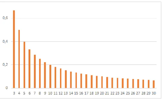
Theorem 1: 𝐹𝑜𝑟 𝑠𝑖𝑚𝑢𝑙𝑡𝑎𝑛𝑒𝑜𝑢𝑠 𝑢𝑠𝑒 , ∀𝛼, ∃𝑛 ̂ (𝛼) 𝑠𝑢𝑐ℎ 𝑡ℎ𝑎𝑡 ∀𝑛 ≥ 𝑛 ̂ (𝛼), 𝐸[𝑐𝑛] 𝑖𝑠 𝑐𝑜𝑛𝑣𝑒𝑥 𝑖𝑛 𝑛 Graph 3 displays the value of α as a function of 𝑛 ̂ (2 ≤ 𝑛 ̂ ≤ 30). When α is higher, E(cn) becomes concave for lower n. Note that E(cn) cannot be concave for n<3. Indeed, E(cn) is null for n=0 or 1, and strictly positive for n=2. For α=2/3, concavity of the number of exposure is verified for all n higher than 3. For α =0.1, concavity is verified for all n higher than 10.
Graphique 3: values of α determining the concavity threshold 𝒏 ̂
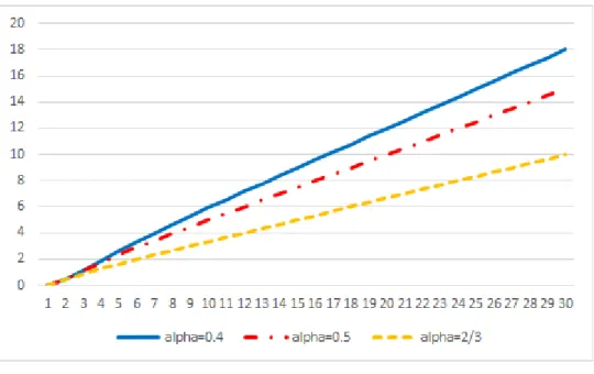
Thus, in this framework, reducing variance is only efficient for low values of α and n. Whether reducing variance can be detrimental (rather than only inefficient) depends on the degree of concavity. Graph 4 displays the exposure curves for the simultaneous case.
Graph 4: expected number of exposures to a contaminated device, depending on the number of users and the proportion of unknown contaminated users (simultaneous use)
0 5 10 15 20 25 1 2 3 4 5 6 7 8 9 10 11 12 13 14 15 16 17 18 19 20 21 22 23 24 25 26 27 28 29 30
alpha=0.01 alpha=0.02 alpha=0.05
0 5 10 15 20 25 30 1 2 3 4 5 6 7 8 9 10 11 12 13 14 15 16 17 18 19 20 21 22 23 24 25 26 27 28 29 30
Graph 4 (continued)
The curves crossing in the graph for α equal to 0.1, 0.2 and 0.5 reflects that as α increases, a higher proportion of people are already sick and thus cannot be contaminated.
For high values of α, concavity is only limited, and for large n, the curves converge to affine functions so that there is not much to lose or gain locally from concavity. This is why the negative values in Table 3 are low in absolute terms, especially for intermediate values of n (that is, for the same deviations as those presented in Table 1).
Table 3: relative increase in the number of expected exposures due to mean-preserving deviations
α
Small n Intermediate n global
3 +/- 1 3 +/- 2 4 +/- 1 4 +/- 2 6 +/- 3 10 +/- 5 20 +/- 10 10 +/- 9 0.001 16.6% 66.5% 8.3% 33.2% 29.8% 27.5% 25.8% 89.1% 0.002 16.6% 66.3% 8.3% 33.1% 29.7% 27.3% 25.3% 88.3% 0.005 16.5% 65.8% 8.2% 32.8% 29.2% 26.5% 23.8% 85.8% 0.01 16.3% 65.0% 8.0% 32.2% 28.4% 25.2% 21.5% 81.8% 0.02 15.8% 63.4% 7.8% 31.0% 26.8% 22.8% 17.4% 74.2% 0.05 14.6% 58.5% 6.9% 27.7% 22.4% 16.5% 8.1% 54.9% 0.1 12.6% 50.8% 5.6% 22.6% 15.9% 8.5% 0.3% 31.8% 0.2 8.9% 36.7% 3.3% 13.6% 6.2% -0.1% -2.1% 7.8% 0.3 5.5% 24.2% 1.4% 6.4% 0.3% -2.6% -0.9% -1.2% 0.4 2.5% 13.3% 0.0% 1.0% -2.7% -2.3% -0.2% -4.0% 0.5 0.0% 4.2% -0.9% -2.7% -3.5% -1.4% 0.0% -4.8% 2/3 -2.8% -7.4% -1.3% -5.1% -2.4% -0.3% 0.0% -5.0%
Closer examination of the exposures formulas and curves reveals two facts. First, for high α, concavity occurs mainly for very low n, since for higher n the exposure curves converge very fast toward affine functions. Second, for high α, the slope of the latter affine functions is rather flat. The combination of initial concavity and subsequent flat slope provides scope for global concavity.
As regards initial concavity, I compute small deviations for small n (left part of table 3). For very high α, local concavity can be meaningfull. For instance, having one person in a room and five in another reduces exposures by 7.4% with respect to the three/three organization. Still, the reverse holds, and with much larger difference, when α is lower than 0.4.
As regards global concavity, I compute large deviations presented in the last column of table 3. Concavity can be meaningful : having one person in a room and 19 in another reduces exposure by 5% if α=2/3. Note that this result only means that all people in the “big” room are exposed for sure, while the lonely one is not. Still, the reverse holds for α lower than 0.2, with larger benefits for equal distribution. Gains can be substantial for small n and small changes in n. Note that in the simultaneous use case, implementing precise small changes in n is realistic in many settings.
As a conclusion, although local and global concavity exists for simultaneous use with high values of α, this concavity is much less meaningful than the convexity observed for lower α. Overall, and except if α is known to be very high, reducing the variance of simultaneous occupation of offices and other rooms is beneficial. Still, concavity above a threshold which decreases with α provides further argument for early organizational action during an epidemic.
6. Additional effect of multiple spreaders
6.1 Successive use when the probability of contamination increases with the number of spreaders I have considered the case where the probability of contagion depends only on the fact that at least one previous user is already contaminated. But the number of users may also have an effect. If 𝛽 ≤ 1
𝑛 − 1
⁄ , the conditional contamination rate can be approximated with the linear probability model in which each spreader increases linearly the probability of contamination. In this case, for 1<=i<n, user i+1 is exposed to a number of previous spreaders which is:
[11] 𝐸[# 𝑠𝑝𝑟𝑒𝑎𝑑𝑒𝑟𝑠(𝑖)] = ∑ 𝑗. 𝐶𝑖𝑗𝛼𝑗(1 − 𝛼)𝑖−𝑗 𝑖
𝑗=1
Where 𝐶𝑖𝑗 =𝑗!(𝑖−𝑗)!𝑖! . Thus, the expected number of new contaminations when n users use successively a device is: [12] 𝐸[𝑐𝑛] = 𝛽(1 − 𝛼) ∑ ∑ 𝑗. 𝐶𝑖𝑗𝛼𝑗(1 − 𝛼)𝑖−𝑗 𝑖 𝑗=1 𝑛−1 𝑖=1 Where β is defined by equation [3]. The sum over j is the computation of the expected value of the binomial distribution В(i,α), which is equal to iα, so that:
[13] 𝐸[𝑐𝑛] = 𝛽(1 − 𝛼) ∑ 𝑖𝛼 𝑛−1 𝑖=1 = 𝛽𝛼(1 − 𝛼)(𝑛 − 1)(𝑛 − 2) 2
Thus [13] is a parabola, is convex and actually more convex than [5] for large realistic values of n. This provides additional argument to decrease the variance of n. Of course, decreasing the expected n remains a first best, whenever possible.
Table 2: relative increase in exposure due to a mean-preserving deviation of n/2
n 6 10 20
45.0% 34.7% 29.2%
Note that with linear probabilities, the relative gains do not depend upon α. However, linear probabilities are considered here for tractability. If α is high, the number of spreaders increases quickly with n so that, unless β is arbitrarily low, linear probabilities quickly sum above one. With logit or probit probabilities, which may be more realistic in many setups, the relative effects may be slightly lower, but are likely to depend on α, as in the baseline case presented above.
6.2 Simultaneous use when the probability of contamination increases with the number of spreaders The risk of contamination is likely to increase with the simultaneous number of spreaders in a room. If 𝛽 ≤ 1 𝑛 − 1⁄ , the risk of contamination can be approximated with the linear probability model in which each spreader increases linearly the probability of contamination:
[17] 𝐸[𝑐𝑛] = 𝛽 ∑ 𝑖. (𝑛 − 𝑖)𝐶𝑛𝑖(1 − 𝛼)𝑖 𝑛−1 𝑖=1 𝛼𝑛−𝑖 = 𝛽 ∑ 𝑖. (𝑛 − 𝑖)𝐶𝑛𝑖(1 − 𝛼)𝑖 𝑛 𝑖=1 𝛼𝑛−𝑖 = 𝛽𝑛 ∑ 𝑖. 𝐶𝑛𝑖(1 − 𝛼)𝑖𝛼𝑛−𝑖 𝑛 𝑖=1 − 𝛽 ∑ 𝑖2𝐶 𝑛𝑖(1 − 𝛼)𝑖𝛼𝑛−𝑖 𝑛 𝑖=1 where β is defined by equation [4]. The two sums correspond to the first and second moments of a binomial distribution Β(n, 1-α). Thus:
𝐸[𝑐𝑛] = 𝛽𝑛2(1 − 𝛼) − 𝛽[𝑛𝛼(1 − 𝛼) + 𝑛2(1 − 𝛼)2] which, after a series of simplifications, gives
[18] 𝐸[𝑐𝑛] = 𝛽𝛼(1 − 𝛼)𝑛(𝑛 − 1) and therefore:
[19] 𝐸[𝑐𝑛] − 𝐸[𝑐𝑛−1] = 2𝛽𝛼(1 − 𝛼)(𝑛 − 1) [19] is increasing in n so that [18] is convex (which is also directly noticeable). Note that [19] can be obtained by direct combinatory reasoning. Over a sample of n-1 users, on average there are (n-1)(1-α) healthy people, and the nth user is a spreader with probability α, so that with the linear probability model, the increase in contamination over the n-1 first users due to the arrival of user n is 𝛽𝛼(1 − 𝛼)(𝑛 − 1). Furthermore, over the first n-1 users, the expected number of spreaders is (n-1)α and the nth is healthy with probability (1-α) so that he gets contaminated with probability 𝛽𝛼(1 − 𝛼)(𝑛 − 1). The addition of both effects provides equation [19].
7. Robustness and limitations
7.1 Robustness and misspecification
The convexity results presented here are quite general. In particular, they must be taken into account in the dynamic case: even with repeated uses, at each time the cross-section variance of n must be kept low.
The framework used in the present paper assumes that all non-spreaders are susceptible to contamination. The extension to a SIR-like model where healed people are immune is straightforward: either immune people are known, and they must be excluded from computation, or only their proportion is known. In the latter case, let h be the proportion of immune (healed) people in the population of non-spreaders. Then [5] becomes:
[20] 𝐸[𝑐𝑛] = 𝛽(1 − 𝛼)(1 − ℎ) ∑(1 − (1 − 𝛼)𝑖−1)
𝑛
𝑖=2
Equations [5], [6] and [7] are modified accordingly, as well as equations [12] to [20]. Equations [9] and [10] are left unchanged. Note that for the sake of simplicity, I have defined h as a proportion of non-spreaders, not as a proportion of the total population. Conversely, if h affects the proportion of spreaders, all equations must be modified accordingly.
7.2 Variance of the contamination rate and probability of an outbreak
Reducing the variance of exposure in order to slow contagion is a new idea. Actually, in a slightly different context, Lipsitch et al. (2003) show that for a given average rate of contamination (number of people infected by each spreader), if the number of cases in the total population is limited to a handful, then a higher variance of the contamination rate reduces slightly the probability of an outbreak. Given this apparent contradiction, the difference between the present framework and the analysis of Lipsitch et al. must be explained.
First, the decrease in the probability of an outbreak identified by Lipsitch et al. is quantitatively limited, and relies on the fact that the number of cases in the total population is very limited: with ten spreaders, an outbreak is almost certain whatever the variance.
Second, and more importantly, a higher variance reduces the probability of an outbreak but not the expected number of contaminated people. Actually, Lipsitch et al. document that over the 201 first SARS cases in Singapore, 103 were contaminated by just 5 people. Thus, there is no real contradiction between the present analysis and that of Lipsitch et al., who do not assert that higher variance would be beneficial in any sense.
8. Conclusion and future research
The homogenous use and cleaning of a limited number of devices used successively by many people limits contamination when some users are unknown contagious carriers of a virus. That is, it is optimal that the same (or at least a very similar) number of people uses each device between two cleanings. This result is based on the fact that when many people use the same device, the probability that some of them are infected increase and the number of people they can infect also increases, so that the number of exposures to contamination is a convex function of the number of successive users. This result is robust to parameters such as the proportion of spreaders or the conditional probability of contamination. For realistic parameters values at the start of an epidemic, reducing heterogeneity in use and cleaning reduces substantially the speed of contamination. However, for this baseline framework, the effects tend to decrease when the proportion of contaminated people increase. Convexity results extend only partially to the simultaneous use framework, for which I evidence concavity above a number of users that decreases with the proportion of spreaders. This provides additional argument for early organizational action in times of epidemic.
I also consider the case where more spreaders increase the conditional probability of contamination. Convexity tends to increase, at least with the linear probability model. This model, which is used for tractability, may lack realism if the proportion of spreaders is high. Further work, using for instance logit or probit transforms, may be in order here.
Surprisingly enough, these variance considerations, as well as the simple need to reduce the average number of people using a device or sharing a space, are often disregarded even during deadly epidemics. Also, the previous literature points to the beneficial effects of higher variance on the risk of an outbreak, but to the best of my knowledge, not to its detrimental effects on the expected number of contaminations.
Although crucial, these variance considerations are second-order with respect to the need for decreasing the average number of users and more generally to the need for public health policies of social distancing, test and track, or others, in times of epidemic. Their advantage is to be implementable in times of high uncertainty with very scarce information. In later phases, they may help slow contamination and, for instance, make test and trace policies more efficient. Note that if the research question addressed here is the speed of contamination rather than the final steady state, these variance considerations could be embedded in a more general framework to assess their contribution to decreasing the contamination rate Rt below one during epidemics.
The meaning of the results presented here depends on the channels of contamination at work in a specific epidemic. Cleaning constraints may be imposed by the ratio of the number of people and uses to the cleaning capacity over a given period. In that case, and if the time span between two users does not matter, the number of devices is of minor relevance. Conversely, if cleaning constraints are time-related (e.g. natural cleaning happens over night as regards aerosol risk of contamination) or if the time-span between two users matters, then increasing the number of devices decreases exposure. These topics deserve consideration in future work.
Dynamic analysis (people using the devices or sharing the offices/production lines repeatedly) is required in future research and may include topics like constant nominal allocation of people to devices and constant running order. The case of different types of devices and the optimal organization with constant nominal allocation (e.g. the potential optimality of having the same and/or nested nominal allocations of a group of people to different types of devices) deserves consideration. 9. references
Alvarez, L. (March 28, 2020), “A model to forecast the evolution of the number of COVID-19 symptomatic patients after drastic isolation measures”, mimeo.
Bai Y, Yao L, Wei T, F. Tian, D.-Y. Jin, L .Chen and M. Wang (February 21, 2020), “Presumed asymptomatic carrier transmission of COVID-19”, JAMA. (Epub ahead of print)
Bernoulli, D. Essai d’une nouvelle analyse de la mortalité causée par la petite vérole. Mem. Math. Phys. Acad. R. Sci. Paris. 1766:1–45
Booth T. F., B. Kournikakis, N. Bastien, J. Ho, D. Kobasa,L. Stadnyk, Y. Li, M. Spence, S. Paton, B. Henry, B. Mederski, D. White, D. E. Low, A. McGeer, A. Simor, M. Vearncombe, J. Downey, F. B. Jamieson, P. Tang and F. Plummer (2005) “Detection of airborne severe acute respiratory syndrome (SARS) coronavirus and environmental contamination in SARS outbreak units”, J Infect Dis. Vol. 191, pp.1472– 1477.
Centers for Disease Control and Prevention (February 29, 2020), “Strategies for Optimizing the Supply of N95 Respirators”,
Chang, D. G. Mo, X. Yuan, Y. Tao, X. Peng, F.Wang, L. Xie, L. Sharma, C. S. Dela Cruz, E. Qin (March 27, 2020), “Time Kinetics of Viral Clearance and Resolution of Symptoms in Novel Coronavirus Infection,”, American Journal of Respiratory and Critical Care Medicine.
Dietz K. and J. Heesterbeek (2002), Daniel Bernoulli’s epidemiological model revisited. Math. Biosci.; vol.180, pp. 1–21.
Doremalen, N. van, T. Buskmaker, D. H. Morris, M. G. Holbrook, A. Gamble, J. L. Harcourt, N. J. Thornburg; S. I. Gerber, J. O. Lloiyd-Smith, E. de Wit and V. J. Munster (March 17, 2020), “Aerosol and Surface Stability of SARS-CoV-2 as Compared with SARS-CoV-1”, New England Journal of Medicine, DOI: 10.1056/NEJMc2004973
Fekom, M., N. Vayatis and A. Kalogeratos (September 9, 2019), “Sequential Dynamic Ressource Allocation for Epidemic Control”, arXiv
Flaxman, S., S. Mishra, A. Gandy, S. Bhatt, N. M. Ferguson, H. J. T. Unwin, H. Coupland, T. A. Mellan, H. Zhu, T. Berah, J. W. Eaton, P. N. P. Guzman, N. Schmit, L. Callizo, K. E. C. Ainslie, M. Baguelin, I. Blake, A. Boonvasiri, O. Boyd, L. Cattarino, C. Civarella, L. Cooper, Z. Cucunubá, G. Cuomo-Dannenburg, A. Dighe, B. Djaafara, L. Dorigatti, S. van Elsland, R. FitzJohn, H. Fu, K. Gaythorpe, L. Geidelberg, N. Grassly, W. Green, T. Hallett, A. Hamlet, W. Hinsley, B. Jeffrey, D. Jorgensen, E. Knock, D. Laydon, G. Nedjati-Gilani, P. Nouvellet, K. Parag, L. Siveroni, H. Thompson, R. Verity, E. Volz, P. G. T. Walker, C. Walters, H. Wang, Y. Wang, O. Watson, C. Whittaker, P. Winskill, X. Xi, A. Ghani, C. A. Donnely, S. Riley, L. C. Okell, M. A. C. Vollmer (March 30, 2020), “Report 13 - Estimating the number of infections and the impact of non-pharmaceutical interventions on COVID19 in 11 European countries”, MRC Centre for Global Infectious Disease Analysis.
Kim S. H., S. Y. Chang, M. Sung, J. H. Park, H. B. Kim, H. Lee, J.-P. Choi, W. S. Choi, and J.-Y. Min (2016), “Extensive viable Middle East respiratory syndrome (MERS) coronavirus contamination in air and surrounding environment in MERS isolation wards”, Clin Infect Dis. Vol. 63, pp.363–369.
Kupferschmidt, K. and J.Cohen (Mar. 2, 2020 ), “China’s aggressive measures have slowed the coronavirus. They may not work in other countries”, Science
Leung, N. H. L. C. Xu, D. K. M. Ip, and B. J. Cowlin (November 2015), “The fraction of influenza virus infections that are asymptomatic: a systematic review and meta-analysis”, Epidemiology; vol. 26, n°6, pp 862–872. doi:10.1097/EDE.0000000000000340
Li, Q., X. Guan, P. Wu, X. Wang, L. Zhou, Y. Tong, R. Ren, K. S. M. Leung, E. H. Y. Lau, J. Y. Wong, X. Xing, N. Xiang, Y. Wu, C. Li, Q. Chen, D. Li, T. Liu, J. Zhao, M. Liu, W. Tu, C. Chen, L. Jin, R.Yang, Q. Wang, S. Zhou, R. Wang, H. Liu, Y. Luo, Y. Liu, G. Shao, H. Li, Z. Tao, Y. Yang, Z. Deng, B. Liu, Z. Ma, Y. Zhang, G.Shi, T. T. Y. Lam, J. T. Wu, G. F. Gao, B. J. Cowling, B. Yang, G. M. Leung and Z. Feng (January 31, 2020), “Early Transmission Dynamics in Wuhan, China, of Novel Coronavirus–Infected Pneumonia”, New England Journal of Medicine, DOI: 10.1056/NEJMoa2001316
Lipsitch, M., T. Cohen, B. Cooper, J. M. Robins, S. Ma2, L. James, G. Gopalakrishna, S. K. Chew, C. C. Tan, M. H. Samore, D. Fisman and M. Murray (2003), “Transmission Dynamics and Control of Severe Acute Respiratory Syndrom”, Science, vol. 300(5627), pp. 1966–1970. doi:10.1126/science.1086616 Normile, D. (March 17, 2020) “Coronavirus cases have dropped sharply in South Korea. What’s the secret to its success?”, Science, doi:10.1126/science.abb7566
Omrani AS, Matin MA, Haddad Q, Al-Nakhli D, Memish ZA, Albarrak AM. (2013 ), “A family cluster of Middle East respiratory syndrome coronavirus infections related to a likely unrecognized asymptomatic or mild case”. Int J Infect Dis., vol. 17, pp. 668–72.
Ong, S. W. X.; Y. K. Tan, P. Y. Chia, T. H. Lee, O. T. Ng, M. S. Y. Wong and K. Marimuthu, (March 4, 2020), “Air, Surface Environmental, and Personal Protective Equipment Contamination by Severe Acute Respiratory Syndrome Coronavirus 2 (SARS-CoV-2) From a Symptomatic Patient”, JAMA, doi:10.1001/jama.2020.3227
Rothe, C., M. Schunk, P. Sothmann, G. Bretzel, G. Froeschl, C. Wallrauch,. T. Zimmer, V. Thiel, C. Janke, W. Guggemos, M. Seilmaier, C. Drosten, P. Vollmar, K. Zwirglmaier, S. Zange, R. Wölfel, M. Hoelscher, (March 5, 2020), “Transmission of 2019-nCoV Infection from an Asymptomatic Contact in Germany”, New England Journal of Medicine
Santarpia, J. L., D. N. Rivera, V. Herrera, M. J. Morwitzer, H. Creager, G. W. Santarpia, K. K. Crown, D. M. Brett-Major, E. Schnaubelt, M. J. Broadhurst, J. V. Lawler, St. P. Reid and J. J. Lowe (March 26, 2020), “Transmission Potential of SARS-CoV-2 in Viral Shedding Observed at the University of Nebraska Medical Center”, mimeo
Tellier, R., Y. Li, B. J. Cowling and J. W. Tang (2019), “Recognition of aerosol transmission of infectious agents: a commentary”BMC Infectious Diseases volume 19, Article number: 101
Wilder-Smith,A., M. D. Teleman,B. H. Heng,A. Earnest, A. E. Ling and Y. S. Leo, (2005), “Asymptomatic SARS Coronavirus Infection among Healthcare Workers, Singapore”, Emerging Infectious Disease, Vol. 11, n° 7.
World Health Organization (February 28, 2020), “Rational use of personal protective equipment for coronavirus disease 2019 (COVID-19) - Interim Guidance”
World Health Organization (February 28, 2020), “Report of the WHO-China Joint Mission on Coronavirus Disease 2019 (COVID-19)”.
Zou L., F. Ruan, M. Huang, L. Liang, H. Huang, Z. Hong, J. Yu, M. Kang, Y. Song, J. Xia, Q. Guo, T. Song, J. He, H. L. Yen, M. Peiris and J. Wu (Marc 19, 2020), “SARS-CoV-2 viral load in upper respiratory specimens of infected patients”, New England Journal of Medicine DOI: 10.1056/NEJMc2001737