Benefits of battery-uItracapacitor hybrid energy storage systems

Benefits of Battery-U Itracapacitor Hybrid Energy

Storage Systems

Ian C. Smith

Submitted to the Department of Electrical Engineering and Computer Science on May 17, 2012, in partial fulfillment of the requirements for

the degree of

Master of Science in Electrical Engineering at the

MASSACHUSETTS INSTITUTE OF TECHNOLOGY

June 2012

©

ARCHIVES

OF TE CNLOG7Y

JUL R

LOR17,A

I iS

All rights reserved.

Department of Electrical Engineering and

*--7 j

Computer Science

May 17, 2012 ii

Certified by

Thesis Supervisor: John G. Kassakian Professor of Electrical Engineering and Computer Science

Accepted by

Leslie A. Kolodziejski

Chair, Department Committee on Graduate Students Author

Benefits of Battery-Ultracapacitor Hybrid Energy

Storage Systems

by

Ian C. Smith

Submitted to the Department of Electrical Engineering and Computer Science on May 17, 2012, in partial fulfillment of the requirements for

the degree of

Master of Science in Electrical Engineering

Abstract

This thesis explores the benefits of battery and battery-ultracapacitor

hybrid energy storage systems (ESSs) in pulsed-load applications. It investigates and quantifies the benefits of the hybrid ESS over its battery-only counterparts. The metric for quantifying the benefits is charge efficiency - the amount of energy delivered to the load per unit charge supplied by the battery. The efficiency gain is defined as the difference in charge efficiency between the hybrid and the battery-only

ESS.

A custom experimental apparatus is designed and built to supply the

current control for charging and discharging the batteries, as well as the data acquisition for measuring energy and current output. Experiments are performed on both ESSs under four different pulsed

load profiles:

1. 436 ms pulse period, 10% duty cycle, 8 A pulse amplitude

2. 436 ms pulse period, 25% duty cycle, 8 A pulse amplitude

3. 436 ms pulse period, 10% duty cycle, 16 A pulse amplitude

4. 436 ms pulse period, 25% duty cycle, 16 A pulse amplitude

Circuit models are created to accurately represent the battery and ultracapacitors. These models are used in simulations of the same test cases from the physical experiments, and efficiency gains are compared. The circuit models differed from the experimentation by

less than 1%.

with demonstrated gains between 10% and 36%. These benefits were

greatest for the 16 A, 10% duty cycle test case because it combined

the highest pulse amplitude and the shortest duty cycle. It is concluded that high-amplitude, low duty cycle, and low period

pulsed-load profiles yield the highest efficiency gains.

Thesis Supervisor: John G. Kassakian

Acknowledgements

I have many people to thank for making my time at MIT an amazingly rich and rewarding experience.

I would like to first thank my thesis advisor - Professor John Kassakian - for his immense amount of knowledge, wisdom, and patience. Having access to such an outstanding and distinguished MIT professor

has been an amazingly educational experience, and has undoubtedly bolstered my growth as an engineer and as a person. I must also

extend thanks to Professor Joel Schindall for mentoring me throughout

the project. His cool-headed voice of reason and industry experience

has pulled me back onto the right path too many times to count.

I would also like to thank the other members of the LEES community. It takes a lab to raise an engineer and I feel incredibly fortunate to

have had 2 years in LEES. A special thanks, in particular, is due to the

following people for always being there to help me in a time of need

and to keep the mood light when it was getting too dark: Sam, Justin,

Richard, Andy, Minjie, Jackie, Wardah, and Juan. Thank you, Dave Otten, for being a levelheaded voice of reason during all of the chaos. And thank you to everybody else in 10-061 and 10-050 for some memorable moments and good times.

To my parents, I cannot thank you enough for always supporting me. Your advice and love have always kept me on the right course and I am proud to say that I am your son. May this thesis serve as a dedication to the values that I learned from both of you. Thank you Gordon and Alan for being wonderful brothers and always, always

having a joke ready to keep the laughter flowing.

And finally, I would like to thank Dan, Brian, Jose, Matt, Tony, and everybody else at Nest for giving me the opportunity to return for my

degree and for creating a wonderful place to call home after its completion. I could not be more excited for the future and what it

Contents

1

1.1 GENERAL CHARACTERISTICS OF ULTRACAPACITORS... 12

1.2 A BRIEF HISTORY OF ULTRACAPACITORS... 16

1.3 PRIOR RESEARCH AND APPLICATIONS ... 17

1.4 THESIS OVERVIEW ... 20

2 - EXPERIM ENTATION ... 23

2.1 HARDWARE DESIGN ... 26

2.2 CALIBRATION AND DATA PROCESSING... 35

2.3 ANALYSIS AND RESULTS ... 44

2.4

3 - SIMU LA TION... 51

3.1 ULTRACAPACITOR CIRCUIT MODEL ... 52

3.2 BATTERY CIRCUIT MODEL ... 58

3.3 HYBRID ESS CIRCUIT MODEL ... 65

3.4 SIMULATION PROCEDURE ... 67

3.5 SIMULATION RESULTS... 69

3.5

78

4 - CONCLUSIONS AND SUGGESTIONS FOR FUTURE WORK... 79

4.1 CONCLUSIONS ... 79

4.2 SUGGESTIONS FOR FUTURE W ORK ... 81

BIBLIOGRAPHY... 85

APPENDIX A ... 89

APPENDIX B... 123

APPENDIX C... 163

List of Figures

Figure 1. Ultracapacitor structure [6]... 14 Figure 2. The ultracapacitor and NiMH battery cell used in the ESS ....24

Figure 3. Test rig block diagram ... 27

Figure 4. High-current circuitry and control. Discharge circuitry is highlighted in blue, charge in orange, and the energy storage

system is highlighted in green... 29 Figure 5. ADC m easurement nodes... 31 Figure 6. Op amp scaling circuits and their scaling constants...31 Figure 7. Battery voltage and temperature during a constant-current

charge. The vertical line denotes the time at which charging

c e a se d ... 33

Figure 8. The test rig PCB layout. The red traces are on the top layer,

the large blue planes are the inner ground layer, and the small blue traces are on the bottom layer. The inner power layer is

h id d e n ... 34

Figure 9. Example calibration of pulse-high and pulse-low scenarios for an 8 A, 25% duty cycle pulse. The blue data points represent the test rig sampling points. The green line is data from the

o scillo sco pe ... . . 38 Figure 10. Data output stream structure ... 40 Figure 11. Plot of the sampling times, overlaid on top of a current

p u ls e ... 42

Figure 12. A single ultracapacitor circuit model...53 Figure 13. Comparing the original ultracapacitor model to experiment

during a long-term charge test... 55 Figure 14. Comparing the original ultracapacitor model with calculated

values to the experimental discharge pulses ... 56 Figure 15. Comparing the four-branch ultracapacitor model simulation

to experimental data in a 10A pulsed discharge test...58 Figure 16. Initial Panasonic Nickel-metal Hydride Battery circuit model

... 5 9

AV

Figure 17. Calculating battery ESR. rESR ~~ ... 60

AI

Figure 18. Battery setting voltage to find the transient branch

re sista nce s ... . 60 Figure 19. Comparing the two-branch battery model to experimental

d a ta ... 62

Figure 21. Comparing the three-branch battery model to experimental d a ta ... . . . 64 Figure 22. Hybrid ESS model with 1 battery pack in parallel with 3

ultracapacitors in series...65 Figure 23. Comparing the hybrid ESS model to experimental data.

Load voltage is on top, battery current on bottom. ... 66 Figure 24. Numerical Simulation Flowchart for a given time, t...68 Figure 25. Optimizing the pulse variables for efficiency gain. Figure

25a) Pulse duty cycle; Figure 25b) amplitude; Figure 25c) period.

74

... 7

s c rip ts ... 164 Figure 28. Hybrid circuit model during a discrete time step.

List of Tables

Table 1. Ultracapacitor and battery component specs [31]. [32]...24 Table 2. Example unaltered readings from a 16 A 25% duty cycle

current pulse, with the data comma-separated in Microsoft Excel.41

Table 3. 16 A 25% duty cycle pulse variable multipliers. The 6 rows represent a different sample during a 25% duty cycle pulse...42

Table 4. Same stream of data from Table 2 after multiplying by the

multipliers from Table 3. The values are displayed in volts...43 Table 5. Experimental data results for the short tests... 45 Table 6. 16 A, 10% duty cycle tests, comparing 'short' test results to

the depletion test results (note the difference in units of energy a nd cha rg e )... . . 47 Table 7. Original three-branch ultracapacitor model component

values, based upon the procedure in [34]...54

Table 8. The final component values used for the four-branch

ultracapacitor m odel in Figure 12... 57 Table 9. Component values for the two-branch battery model...62 Table 10. Battery model component values...64

Table 11. Simulation results for the same test cases that were run in

the experim ental chapter... 70 Table 12. Comparing simulated to experimental data outputs ... 72

1 -

Introduction

This thesis investigates the benefits that ultracapacitors bring to

batteries when combined in a hybrid energy storage system.

Specifically, the benefit that this investigation will focus on is the energy efficiency savings, also known as charge efficiency. Charge efficiency was defined as the amount of energy delivered to the load per unit charge supplied by the battery. The hybrid energy storage system (ESS) in this investigation is of the simplest type - shunting

the ultracapacitors across the battery without any power electronics between them. The complementary characteristics of each of these two devices - batteries achieving high energy density and

ultracapacitors achieving high power density - acting together could

enhance certain systems that rely on just one alone. The systems that benefit the most are ones with a low average power, but a very high peak load. Although this thesis does not focus on quantifying extra battery lifetime in hybrid energy storage systems, the efficiency boost

is very closely related to lifetime extension [1]. This thesis will focus

on quantifying that energy efficiency boost by adjusting the variables of pulse amplitude and duty cycle.

Before moving further, I would like to have a word on naming

conventions. The capacitive devices discussed in this thesis are going to be referred to as "ultracapacitors." This is exactly equivalent to

capacitors." The term "supercapacitor" is derived from the name of NEC's first attempt to commercialize the double-layer capacitor technology, in 1979. The product was dubbed the "Supercap" [2],

[3]. Ten years later, in 1989, the Pinnacle Research Institute of

Cupertino, CA developed a new double-layer capacitor with a more conductive substrate and surface coating, allowing for higher currents

and higher power densities than the Supercap. To distinguish their

new technology from the Japanese competition, Pinnacle applied the

next-highest modifier and marketed the new product under the term

"ultracapacitor" [4]. In modern technical papers, the names refer to

the same type of device with no distinction among them [3], [5]. It is

a matter of the author's preference which one he uses and mine is for

the term "ultracapacitor."

1.1 General Characteristics of Ultracapacitors

Ultracapacitors are structured differently from film and electrolytic

capacitors. Film capacitors, such as multi-layer ceramic capacitors, are the most basic type of capacitor - two conductive parallel plates, separated by an insulating dielectric material. The capacitance

function for this simple capacitor is given by (1), where E is the

dielectric constant, A is the plate area, and d is the distance between

the plates.

C=(1)

d

Electroytic capacitors utilize an electrolyte paste (typically applied to

the cathode) and an oxide layer (typically anodized onto the anode) to

as the dielectric, is much thinner than film capacitor dielectric barriers;

so electrolytic capacitor capacitances can be much higher than film

capacitors. Capacitance varies proportionally to E, and so a great amount of research and work has been placed into finding/creating new insulating dielectrics to increase the energy storage of traditional

capacitors.

Ultracapacitors, however, do not rely on dielectrics to increase their

capacitance. The common techniques are focused, instead, on

increasing A and decreasing d in (1). Figure 1 displays a typical ultracapacitor structure - two porous electrodes separated by a very

thin separator. The electrodes are not smooth, but are porous (activated) carbon. Activated carbon has on the order of 100,000 times the surface area of a smooth electrode, and this is applied to the

variable A in (1). The charge is stored in the thin charge separation

between the carbon electrode and the aqueous electrolyte. This surface between the electrode and electrolyte is known as the

layer. A typical ultracapacitor structure utilizes two of these

double-layers (one at each electrode) separated by thin porous separator,

rtga" charge cojector electrode separator v electrotyte

pos"

++e

eiecrde

Figure 1. Ultracapacitor structure [6]

The downside is that these devices cannot handle voltages as high as

electrolytic capacitors. The electrolyte breaks down at much lower

voltages than an electrolytic capacitor can withstand. Ultracapacitors

have a typical rated voltage of only 2.5 V, which can be 100 times

lower than an equally sized electrolytic capacitor. This voltage rating

can limit the versatility of ultracapacitors, and is a serious challenge

when trying to design them into systems.

The appeal of ultracapacitors is in their high specific power and

extremely high cycle life, when compared to batteries.

The

capacitance of an ultracapacitor can be extremely high, being

measured in the range of Farads, as opposed to microfarads, which is

more typical of an equally sized electrolytic capacitor. The energy

stored in a capacitor increases linearly with capacitance, so

ultracapacitors can be used for much higher energy applications than traditional capacitors could be considered for. An ultracapacitor's ESR is generally lower than that of an equally sized battery, which provides the opportunity for higher currents and very high power densities.

Ultracapacitors are also much more environmentally friendly than any

modern battery; they are typically made of activated carbon plates

with a thin separator, and are usually RoHS compliant, meaning they

have none or trace amounts of lead, mercury, cadmium, and other

toxic materials [7], [8]. They store charge in an electric field, instead of a chemical reaction, so they do not require hazardous materials like

strong acids. The downside of ultracapacitors comes with their relatively low energy density (compared to batteries). For many applications, they do not store enough energy to warrant use without a

main energy source, typically a battery [9]. In other words, they have

mostly been seen as a backup source of power rather than a main source of energy.

A quick comparison between two commercial devices will illustrate this point. Take, for example, a D-Cell-sized ultracapacitor with a

capacitance of 310 F and a safe operating voltage of 2.7 V. This ultracapacitor may nominally store up to 0.3 Wh of energy. Compare

this to an Energizer. Nickel-Metal Hydride (NiMH) D-cell battery of 1.2 V and 2500 mAh. The battery can store 3.0 Wh. This puts the

volumetric energy density of the ultracapacitor at 10% of that of a commercial NiMH battery. The two devices have roughly equal energy density by mass at 41 Wh/kg. However, the ultracapacitor's ESR is only 2.2 m92 and it has the capability of supplying 828 W to a matched

load. The battery's 11 mQ ESR limits its maximum power output to only 32 W [10], [11].

1.2 A brief history of ultracapacitors

Standard Oil first patented Ultracapacitors in 1966 after discovering the technology as a byproduct of their fuel-cell research. Both Standard Oil and GE discovered a highly increased capacitance in carbon electrodes for fuel cells and novel batteries. This occurred due to the storing of charge in what became known as the 'double layer.' They first reached the market in 1978, when Standard Oil licensed the technology to Tokyo-based NEC Corporation, who sold it under the name "Supercap." The first application of ultracapacitors was to provide backup power for computer memory

[2], [3].

The 1970s saw extra research in this field, which yielded sold-state electrolytes. These capacitors were marketed by Gould Ionics but were incredibly expensive and had a low operating voltage. A kind of 'pseudocapacitor' was developed in the 1980s, which stored charge in the 'double layer' in addition to faradaic reactions, much like a battery

[3]. The demand for high-power devices in the 1990s through today

has lead to the rise of high-voltage electrolytes and more advanced technologies [3]. Modern ultracapacitors are being considered more and more for tackling the problems presented by the growth of the hybrid and electric vehicle (HEV and EV) industry [12], [13]. Research is also being conducted into using ultracapacitors for the future electric

grid, where energy storage may become the key for incorporating distributed generation into the network [14].

1.3 Prior research and applications

Research into ultracapacitors for use in hybrid/electric vehicles has

been ongoing for decades [15], [16], [17]. This is because electric

vehicles are the model applications in which scientists and engineers

propose ultracapcitors are beneficial. Electric vehicles require high energy in order to run for a sufficient amount of time, but also high

power for acceleration and braking. One of the most unique

applications of ultracapacitors in vehicles is their use in capturing the

energy normally lost during braking - a practice termed 'regenerative

braking.' This entails using an electric motor that, when it slows down

the wheels, directs the energy into the ultracapacitors, where it would be stored to charge the battery or provide the power necessary for the next acceleration boost [18], [19]. Others have focused on extending

battery lifetime in HEVs with the use of ultracapacitors - a worthy

topic when you consider that batteries can be half the cost of an

electric car [20].

Many car-focused papers performed simulations by taking simplified models of ultracapacitors and batteries and running them through

programs of standard drive cycles [16], [12], [21]. Depending on the

assumptions made, some researchers fail to justify the current cost of

ultracapacitors while others see much promise in the technology [12],

[21], [22]. Other researchers have taken components and actually performed real experiments with the same drive cycles and measured

energy losses and efficiencies [17]. So far no experiment has

provided a conclusive answer to the question of how to efficiently and

economically incorporate ultracapacitors into HEVs and EVs. That is not to say batteries are the only devices with high energy density that is being investigated for use with ultracapacitors. Fuel

cell-ultracapacitor hybrids have also been under research for many years [23], [1].

Other research has been conducted on hybrid energy storage systems without a focus on vehicular applications. Many of these studies go

back to the fundamental principles of whether the combination of

ultracapacitors and batteries are indeed worthy of combining into a hybrid energy storage system. There are a number of researchers

focusing on improving battery lifetime with hybrid energy storage systems [24], [25]. More often than not, however, these experiments

are nothing more than simulations and do not use real components

-only simplified models [5], [26].

Many engineers have designed hybrid systems to utilize both the high power density of the ultracapacitors and the high energy density of the battery simultaneously. With the use of power electronics and active

switching between the two energy sources, it has been shown that adding an ultracapacitor to energy storage systems can indeed take

some of the stress off the battery by sharing the current load [27]. Few, however, have simulated or experimented with batteries that utilize ultracapacitors shunted across the terminals, without power electronics in between them [5], [24], [28].

Three sources - [5], [24], and [28] - have all performed research that is very similar to this investigation. They utilized pulsed loads and

direct-parallel connections between the battery pack and the

ultracapacitors to create hybrid ESSs. However, these works all displayed key differences with this investigation. Reference [5] reports similar pulse-load experiments, but only in simulation and with no physical experimentation. The battery and ultracapacitor models used were the idyllic 'ESR-only' models that gave a basic first-order

approximation of actual results. Reference [24] describes physical

tests with a lithium-ion laptop battery and ultracapacitors using a pulsed discharge load. The battery-only ESS runtime was compared to various hybrid ESS setups: 2 ultracapacitor branches in parallel with the battery; 4 ultracapacitor branches in parallel with the battery; 4 ultracapacitor branches in parallel with and an inductor in series with

the battery; and ultracapacitors separated from the battery by a

DC/DC converter. The pulsed load profile was the same among all of these experiments, which is in contrast to the investigation presented in this thesis.

Reference [28] focused on transient load suppression - maintaining steady voltage during short, heavy loads. The key metric being measured was the voltage droop as a result of a transient current load, as opposed to the charge efficiency and energy availability presented in this thesis. Battery runtime experiments were run on

Li-Ion batteries, which were charged to 4.2 V and then discharged by current pulses until the ESS reached 3 V. The current pulses had an

amplitude of 2 A with a pulse period of 4.61 ms and a duty cycle of 12.5%. The hybrid ESS lasted 2.53 hours while the battery-only ESS

[24], there was no attempt to correlate benefits with the load

characteristics.

1.4 Thesis Overview

This thesis will investigate the benefits that ultracapacitors bring to

batteries when combined in a hybrid energy storage system.

Specifically, the benefit that this investigation will focus on is the energy efficiency savings, also known as charge efficiency. Charge

efficiency is defined as the amount of energy delivered to the load per unit charge supplied by the battery. These savings can be linked to other performance enhancements of batteries, most notably extended

cycle life [29], [30]. There are many topologies to create such a hybrid energy source, some of which require expensive power

electronics and complex control systems. This investigation will

explore the opposite route - that of a battery directly in parallel ('shunted') with ultracapacitors. This is an important distinction from other research - see [26], [18], [19], and [14], which are just some of the references which utilize power electronics to separate the battery

and the ultracapacitors. The direct-parallel system is the simplest

hybrid system, but one that has had relatively little experimental exploration. Some references that explore this are [5], [24], and

[28], as discussed above.

The tests presented in this thesis consisted of applying a pulsed current load on the energy storage system and measuring the energy delivered to the load as well as the charge drawn from the battery,

between the battery-only and the hybrid energy storage systems to determine the benefit of the hybrid system over the battery-only system. This test was performed for two different pulse amplitudes and two different duty cycles, providing four different test cases.

While the results of the four test cases are based upon short tests, the best test case was also validated by cycling a battery to full discharge

to observe if the total available energy from the battery was increased.

The primary method of investigation is presented in Chapter 2. This investigation was experimental in origin, working with commercial batteries and commercial ultracapacitors and known load profiles in

order to draw the conclusions. The load discharge equipment was custom designed and built in order to precisely draw the desired

current profiles and measure the important variables of the energy

storage system. An overview of the design of the board will be included in the chapter, as well as the details of the system calibration, measurement acquisition techniques, and experimental results.

Theoretical examination and simulation are presented in Chapter 3.

The purpose of that chapter is to explore the math and theory behind the investigation in order to support the results obtained in experimentation. It is important to use theory to predict physical

outcomes, because experiments without theoretical backing hang in

question over whether or not lurking variables distorted the intended

results. The ultracapacitor and battery models are simplified to make the solution tractable within a reasonable timeframe, but the load profiles and system losses are characterized as the experiment was actually set up.

Thesis conclusions and suggestions for future work are detailed in Chapter 4.

2

-

Experimentation

This chapter describes the details of the physical experimentation aspect of this investigation. The experiments focused on stressing a hybrid energy storage system (ESS) and a battery-only ESS with

pulsed discharge current loads and measuring the charge efficiency of

each system. The charge efficiency was defined as the amount of energy delivered to the load per unit charge drawn from the battery.

These efficiencies were measured for various pulse profiles in order to determine a pattern that could be generalized for ultracapacitor-based designs. Once measured, the efficiency gain was calculated by

comparing the hybrid ESS to the battery-only ESS to quantify the

added benefit of the ultracapacitors.

All of the tests used one type of battery and/or ultracapacitor. The ultracapacitor used was the Maxwell BCAP0025, with 25 F capacitance

and a rated voltage of 2.5 V. The battery pack consisted of 5

Panasonic Nickel-Metal Hydride HHR379AH cells, with a unit cell voltage of 1.2 V and a rated capacity of 3.5 Ah. The battery pack, which was the same for the hybrid and battery-only ESS, had a

nominal voltage of 6.0 V. This meant 3 ultracapacitors had to be

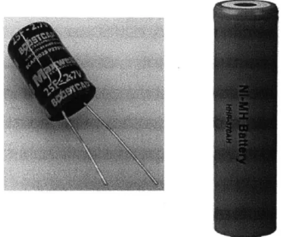
placed in series to maintain their voltages within rating. Pictures of the two energy components are shown in Figure 2; the relative sizes

are not to scale. The dimensions and electrical specs are shown in

Figure 2. The ultracapacitor and NiMH battery cell used in the ESS Table 1.

Ultracapacitor

_Battery

Length (mm)

26

67

Diameter (mm)

16

18.2

Nominal Voltage (V)

2.5

1.2

Capacitance (F)

25

-Capacity

(Ah)

3.5

Series

Cells in

ESS

3

5

Ultracapacitor and battery component specs [31], [32]

A large part of the experimental setup was designing and building the

arbitrary load and measurement equipment. The choice to create the test rig was largely driven by budgetary concerns, rather than design needs. There are commercial solutions that would allow others to perform these experiments without this exact setup, but they come at a price. Recommendations for improvement are discussed more in Chapter 4.

The equipment design was based around the Atmel ATmega168

microcontroller for control and measurement. The microcontroller

sported an 8 MHz internal clock, which was important, as the chip had

to perform many functions in a short time. These functions included

setting the load current, taking measurements of all 8 ADC channels,

and communicating the output data to the computer. The computer

was there only to receive the data and store it in a text file for post-processing.

The controller had the capability of setting arbitrary pulse amplitudes and duty cycles to run various test conditions. The goal of this thesis was to investigate the advantages of ultracapacitor-battery hybrid energy storage systems at the basest level. Any results from this

investigation are meant to act as a guide for future research and to provide a direction for when and how to design ultracapacitors into battery-powered systems.

2.1 Hardware design

The experimental apparatus had to meet a number of important specs. First, it had to be able to handle the high currents expected in this experiment - upwards of 16 A. Second, it had to be completely

software controllable or programmable so that any desired test case may be run at any time. New test cases must have been able to be added, as well. Third, it had to be able to measure the important voltages and currents at all times of the experiments. And fourth, the test rig must have been able to communicate that data to a computer for post-processing. It was decided that a custom board would be designed to meet all of these specs, rather than purchasing an active current source and a data acquisition unit and integrating them into a single system.

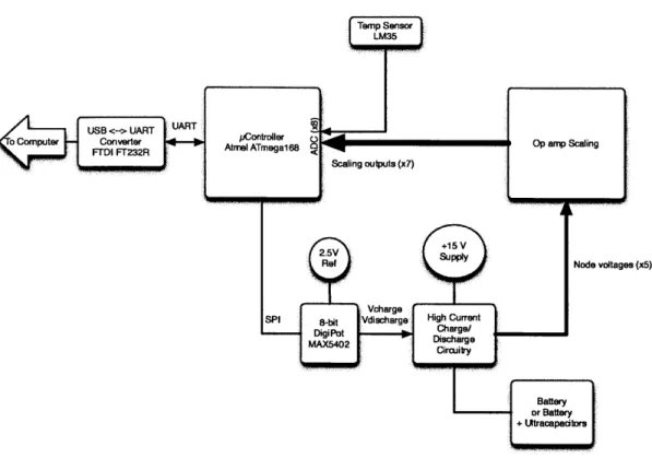
Figure 3 is the block diagram of the test rig. The microcontroller was at the very center of the design and controlled everything on the board. It communicated over a digital Single Peripheral Interface (SPI) bus with a digital potentiometer - the Maxim MAX5402 - in order to generate the proper analog signal to control the current entering or leaving the ESS. These analog signals are labeled Vcharge

and Vdischarge in Figure 3. Final efficiency conclusions were drawn based

upon the data gathered from measuring the node voltages in the high current circuitry. These voltages could not be read directly by the ADC, however, because they were outside the 0-3 V measurement

range. So the signals had to be properly scaled through op amp

scaling circuitry before finally making their way back to the microcontroller's onboard 10-bit ADC.

outputs (x7)

Node voltages (x5)

Figure 3. Test rig block diagram

The high-current charge/discharge and control circuitry are further detailed in Figure 4. This circuitry was designed to give the test rig precise control over the energy storage system current. The circuit

analysis can be split into 3 different sections:

1. The energy storage system (on the right, highlighted in green)

2. The discharge circuitry (bottom left, highlighted in blue)

3. The charge circuitry (top left, highlighted in orange)

The energy storage system can be configured as either a battery-only system or a battery-ultracapacitor hybrid system by either populating or unpopulating one of the ultracapacitors. The discharge circuitry

consisted of a feedback loop operating as a voltage-controlled current

output signal was the voltage across R1. The discharge current from the energy storage system is given by (2).

I., =10*V idb,,, (2)

The feedback path included a 10x multiplier to reduce offset error in U4, in addition to reducing the voltage offset error effect on the function of the circuit. The capacitors and extra resistors in the feedback loop added zeros to increase the loop stability and prevent oscillations. The charge circuitry operated on the exact same principles, except the feedback loop used R2 instead of R1 and it

pushed current into the ESS, rather than pulling current out. R3 was

added as a current sense resistor in order to allow the system to measure the battery current in the hybrid scenario.

Figure 4. High-current circuitry and control. Discharge circuitry is highlighted in blue, charge in orange, and the energy

With the high-current circuitry designed, a microcontroller had to be chosen to control the current. The microcontroller selected for this board was the Atmel ATmega168, with the key features being an 8MHz

internal clock, a SPI interface, and an 8-channel, 10-bit ADC. These

were important for capturing all of the data and controlling the current

in a timely and precise manner.

The current and voltage measurements were performed by reading the

voltages at the key nodes highlighted in Figure 5. Each signal went through a scaling circuit before it got to the ADC of the microcontroller. The purpose of the scaling circuit was to frame the voltage in the 0-3 V range of the ADC. And negative voltages, such as the voltages of the nodes VD2 and VD3 when discharging the battery,

had to be inverted to prevent the ADC from saturating at the low rail. The scaling circuitry is detailed in Figure 6.

Vbatt

VC2ND2

m10

VciND3

Figure 5. ADC measurement nodes

VD2 NC2 VD3 NC1 ADC1 --VD3*2 ADCO Vbatt + Vcap 10k ) _{k3 =b A D C 7} =Vbattl.34 MJM VD1 6.341k l~kflADC6 =VcapI7.34 1 k1 oADC2 =VD1*3

One ADC pin (ADC5) was dedicated to a LM35 temperature sensor, with the purpose of measuring battery temperature. The LM35 was

covered in thermal grease and taped down between two of the five battery cells, in order to thermally couple to the battery as much as possible. The battery temperature was used for two purposes: safety

and battery charging. First, the battery temperature was continuously monitored no matter what the controller was doing at the time. If the

battery temperature reached or exceeded 50 *C then the current was

shut off and all experiments were terminated. Tests that were automatically run back-to-back would also wait for the battery temperature to fall below 25 *C before beginning a new test, so the

batteries would all start relatively cool and at the same thermal state.

Unlike the discharge protocol, which ran for a set amount of time or

pulses, the battery charging protocol contained a firmware feedback

loop which would rely on the battery's temperature to determine when charging was complete. The key metric was not the specific temperature - though it was programmed to shut off if the battery exceeded 50 *C - but the derivative of the charge temperature. The

battery datasheet instructed the battery was fully charged when its temperature rose at a rate greater than or equal to 1*C/minute. So the charging protocol measured the battery temperature every minute

and if it had risen by at least 1 0C from the previous measurement

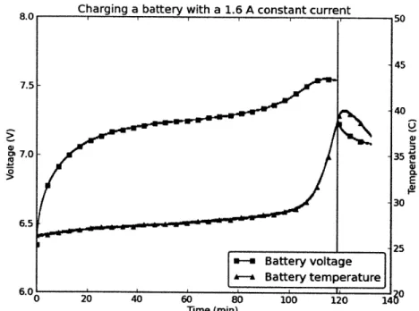
then it would stop charging the battery and let it cool back down to 25 0_{C. A plot of the battery voltage and temperature during a charge} cycle is displayed in Figure 7.

(TV 0 -0 5 .3 E 30 6.5 25 -eBattery voltage

*-i Battery temperature

0 20 40 60 80 100 120 1490

Time (min)

Figure 7. Battery voltage and temperature during a constant-current charge. The vertical line denotes the time at which

charging ceased.

The PCB layout is shown in Figure 8 below. It is a four-layer board

with signals on the outer layers, ground on the second layer, and +15

V and the digital +5 V splitting the third layer. The ADC scaling and

current control circuitry in the low current analog section was laid out mostly on the bottom layer using surface mount parts to keep the board area within the PCB manufacturer's limits. Care had to be taken

in order to properly lay out the ground plane and isolate the high-current circuitry from the low-high-current analog circuitry and the digital circuitry. Notice the cut in the ground plane near the 15V connector at

the bottom of the board - this cut ensured the high current would not circulate through the sensitive low-power analog or digital ground

plane on the left half of the board. The high-current planes were all

the trace impedance low. These aspects were critical to the design, because high trace impedance or ground plane shift would directly affect the voltage across the 1OmQ sense resistors and the ADC

readings.

Figure 8. The test rig PCB layout. The red traces are on the top-layer, the large blue planes are the inner ground top-layer, and the small blue traces are on the bottom layer. The inner

power layer is hidden.

The digital circuitry consisted of support for the microcontroller, as well as the means to program the board and communicate with the computer. The 6-pin header allowed the board to be reprogrammed in-circuit using the Atmel AVRISP MkII programmer. Serial

communication with the computer was made possible with the FTDI FT232R USB-to-UART chip. The downside with this design was the

added ground noise when the USB was connected to the computer. This noise was compensated for in the calibration process, but could have been avoided altogether. This will be discussed more in Chapter

4, with suggestions for eliminating this issue.

2.2 Calibration and data processing

The test rig output the raw ADC data to the computer, which saved it in a text file for post-processing. Like any other piece of measuring

equipment, this data had to be calibrated by comparing the test rig's data to a known reliable source of the same measurements. Calibration was an extremely important aspect of measurement, because without it there would be no confidence in the results drawn from the data. The process of calibration involved adjusting the available variables of the data post-processing algorithms to match a known desired output. These adjustments accounted for minor part-to-part variations in the components, device tolerances, and the board layout. The test rig carried upwards of 16 A flowing on the board; any extra impedance introduced by the traces could cause the ADC measurements to be slightly off. These errors could add up when the test rig took thousands of measurements over the course of one

experiment.

Calibration was performed over each amplitude used 8 A and 16 A -and each duty cycle - 10% -and 25%. Calibrating along current levels was essential, because trace impedance errors would affect

measurements with an offset proportional to the load current.

Calibrating by duty cycle was an extra precaution taken to ensure the data accuracy. The output of the calibration procedure was a series of

multipliers for each variable, which accounted for imperfections in the

system.

The known desired output in this case was recorded by a calibrated

Tektronix DPO 3034 oscilloscope. Measurements were taken at each measurement node in the test rig, and the test rig output its data

stream at the same time. So we had two interpretations of the same

signals - one from the oscilloscope and the other from the test rig. An

important detail to note was that the oscilloscope had only four channels, but there were five variables that needed to be calibrated:

VD, VD2, VD3, Vbatt, and Vcap. So a second calibration cycle was run

immediately following the first to gather data on the variables that were missed in the first run. The assumption was made that the capacity of the battery was high enough, and the battery was always

charged before calibration, that the difference between two consecutive tests was negligible.

Another problem that was encountered while initially performing

calibration tests was the high range of values that could be seen, due

to the pulsed nature of the experiments. The resolution, even on

11-bit Hi-Res mode, for an 8-division vertical scale oscilloscope was not

high enough when the entire voltage ranges had to be taken into

account. Decreasing the vertical scale would increase the measurement resolution, but that would cause the scope to saturate and the measurements would be worthless. The solution was to

waveforms separately. An example of this is illustrated in Figure 9. The blue points indicate the sampling times of the custom controller. It was these points that were compared to the raw controller data for calibration.

SA, 25% Duty Cycle sampling times - pulse high Raw Data Sampling points 0.2 0.4 Time (s) 0.6 0.8 0 Figure 9. to Time (s)

Example calibration of pulse-high and pulse-low scenarios for an 8 A, 25% duty cycle pulse. The blue data points

represent the test rig sampling points. The green line is data from the oscilloscope.

4.2 4.0 3.8 3.6 3.41 C LI 3.2 3.0 2.8 to

The structure of the data output from the test rig is displayed in Figure

10. It consists of 11 data fields, each in a decimal format. The first 6 digits represent the record number, which starts are 0 and increments

by one for every line sent to the computer. This number is used for keeping track of time: the sampling period is a precise 7.382 ms, so the time from start is the record number multiplied by 0.007382. The

next field represents the state of the test rig. The states are defined as:

1 - Controller is in between current pulses 2 - Controller is pulsing current

3 - Controller is currently charging the battery

4 - Controller is waiting for the battery to cool down before beginning to charge the battery (waits until the battery is under 250_C)

5 - Controller is waiting for the battery to cool down before beginning

to discharge the battery (waits until the battery is under 25*C)

The third data field is the magnitude of the commanded current from

the controller at that instant. This number is reported in the units of mA. The next 8 data fields are the 10-bit ADC readings of each of the 8 channels. They are represented from left to right in the numerical

ADC channel order (ADCO on the far left, ADC7 on the far right). The order is as follows: ADCO = Vc2 ADC1 = VD3 ADC2 = VD ADC3 = VD2 ADC4 = Vc2

ADC5 = temp

ADC6 = Vcap

ADC7 = Vbatt

ADC5, the temperature of the battery, was unlike the other

measurements. The LM35 temperature sensor mounted to the battery reported an analog voltage equal to 10 mV for each absolute degree Celsius. It was only recorded in 3 digits, because the environmental conditions were known not to get above 990C or below 0*C, and the microcontroller automatically removed the charge/discharge current from the battery if its temperature rose to 500C or above.

000774,1,0000,0007,0003,0003,0075,0006,210,0815,0819,

ADC outputs

Commanded Current (mA)

* Current state (1=discharge,3=charge)

* Record number

Figure 10. Data output stream structure.

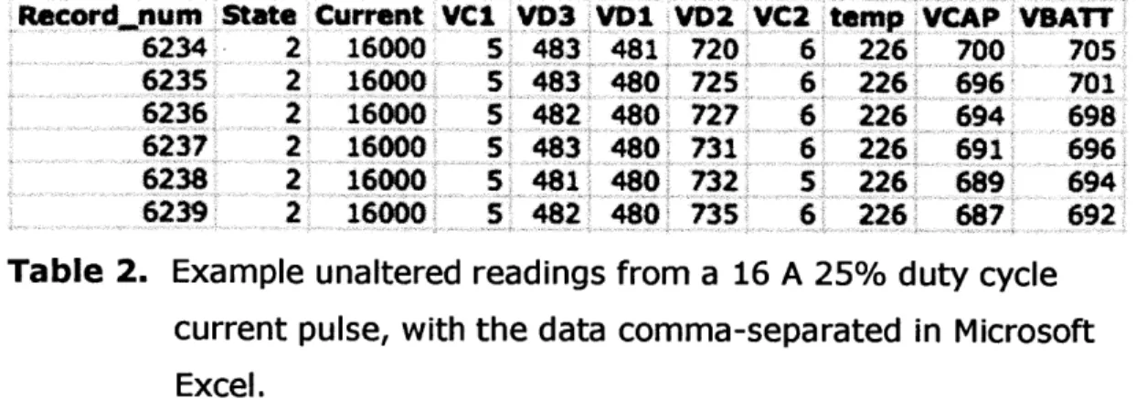
A sample stream of raw data from the test rig, taken during a 16 A 25% duty cycle current pulse, is displayed in Table 2. Short streams

of data (under 10,000 lines) could be analyzed in Microsoft Excel, but larger streams (over 10,000 lines) required a python script similar to those used in Chapter 3 to calculate the simulation results. This

Record.num State Current VC1 VD3 VD1 VD2 VC2 temp VCAP VBATT 6234 2 16000 5 483 481 720 6 226 700 705 6235 2 16000 5 483 480 725 6 226 696 701 6236 2 16000 5 482 480 727 6 226 694 698 6237 2 16000 5 483 480 731 6 226 691 696 6238 2 16000 5 481 480 732 5 226 689 694 6239 2 16000 5 482 480 735 6 226 687 692

Table 2. Example unaltered readings from a 16 A 25% duty cycle current pulse, with the data comma-separated in Microsoft

Excel.

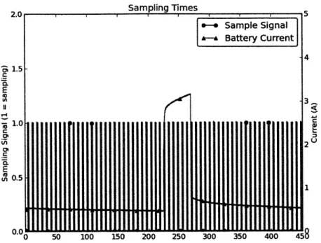
The sample times were well documented and controlled, with a

sampling period of 7.382 ms. The first sample of the pulse occurred 638 ps after the pulse began, ensuring continuity of the data points. A plot of the sampling points vs. the current pulses is displayed in Figure 11. This allowed us to correlate exact scope measurements to each of the pieces of data output from the test rig. The result was a table of multipliers for each of the five variables at each of the -'60 data points captured by the test rig. An example of the 16 A, 25% duty cycle multiplier table is shown in Table 3.

31.5

CLL

S1.0

0* 50 100 150 200 250 300 350 400 458

Figure 11.

Plot of the sampling times, overlaid on top of a current

pulse.

Sample # VD1 mutt VD2 mutt VD3 mutt VCAP mutt VBATT mut 1 0.000345 -0.000354 -0.000371 0.007857 0.007811 2 0.000345 -0.000354 -0.000371 0.007857 0.007813 3 0.000345 -0.000354 -0.000371 0.007855 0.007807 4 0.000344 -0.000354 -0.000371 0.007859 0.007811 5 0.000345 -0.000353 -0.000372 0.007859 0.007814

6 0.000345 -0.000353 -0.000372

0.007857

0.007809

Table 3.

16 A 25% duty cycle pulse variable multipliers. The 6 rows

represent a different sample during a 25% duty cycle pulse.

The multipliers had a twofold operation. The first was discussed above

-

error correction and accounting for an inevitably imperfect system.

The second was converting the ADC number from an ADC value to the

actual voltage at the measured node. That is why the numbers are all

much less than one. The data from Table 2, after converting to voltage

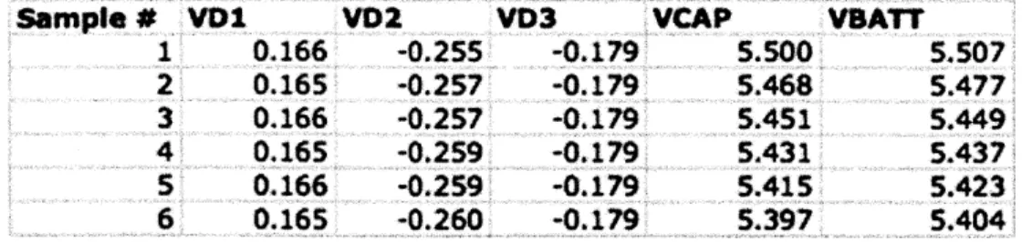
by using the multipliers in Table 3, is displayed in Table 4.

Sample # VD 1 2 3 4 5 6 0.166 0.165 0.166 0.165 0.166 0.165 Table 4. Same stream

multipliers fro VD2 VD3 VCAP VBATT -0.255 -0.179 5.500 5.507 -0.257 -0.179 5.468 5.477 -0.257 -0.179 5.451 5.449 -0.259 -0.179 5.431 5.437 -0.259 -0.179 5.415 5.423 -0.260 -0.179 5.397 5.404

of data from Table 2 after multiplying by the

m Table 3. The values are displayed in volts.

The individual node voltages were all that were needed to calculate the full test results. The conversions from node voltages to current and energy are given by (3) and (4).

IB =(D3 - VD2)

R,

EL =f VAp-!D3 + I -P, +(Va, -V)- IBdt

A R2

(3)

(4)

The energy delivered to the load, EL, lumped the sense resistors and trace impedance in with the load. Essentially, the idea was that

everything that was not the hybrid ESS was considered part the load. The first three terms in (4) included energy waste in the discharge

MOSFET, R2, R2, and R3. The final term accounted for the impedance

between the Vbat and Vcap nodes. The board had the pads to accept a

MOSFET to open the connection between the ultracapacitor bank and

the battery, but those pads were shorted using a jumper and thick-gauged wire. Nevertheless, there existed some impedance between the two nodes and that energy had to be accounted for. For reference, this jumper accounted for less than 0.1% of the total energy counted as "delivered to the load."

2.3 Analysis and Results

All of the data points for each test case culminated in two essential

metrics: the amount of energy delivered to the load (EL) and the amount of charge removed from the battery to deliver that energy (fIB). These parameters were combined to calculate the charge

efficiency - that is, the amount of power delivered to the load per unit charge removed from the battery. This efficiency was given by (5).

Ef B

(5)

This metric was chosen because it has far-reaching implications for the

usefulness of the hybrid ESS. If the charge efficiency is higher in the hybrid ESS than the battery-only ESS then the battery could supply

more energy to the load for less charge. This would mean that a

hybrid ESS could run longer on a single charge than its battery-only

counterpart. Less energy waste would also mean the battery will stay cooler for longer, which has been directly linked to increased battery

lifetime [33].

There were two types of tests run: the 'short' tests and the 'depletion'

tests. The short tests were called such because the data came from sampling just ten pulses - the final ten pulses in a hundred-pulse series. The tests were set up with a 90-pulse buffer because it could

take a little while before the system would reach periodic steady state,

and a short number of pulses would not be subject to the decline in battery voltage as its state of charge decreased. For example, ten 16 A, 435ms, 25% duty cycle pulses would add up to only 0.0019 Ah, or

0.055% of the battery's capacity. The batteries were freshly charged

before beginning these tests, to keep the results as consistent with

each other as possible.

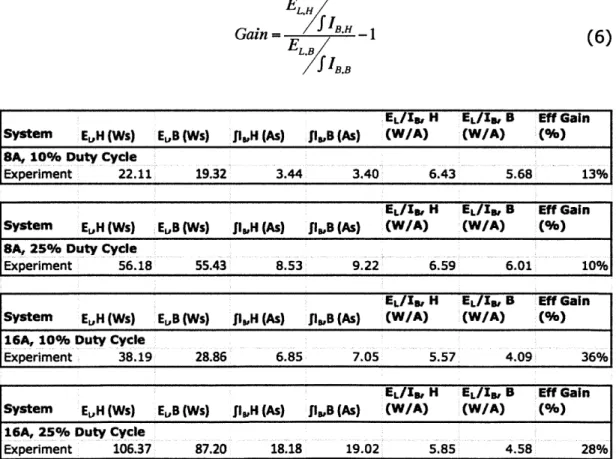
The final summary of the experimental short test results is displayed in Table 5. It is structured to display only the final, important parameters: EL and

JIB

scenarios, their corresponding charge efficiencies ( EI dt I' and the

efficiency gain. increase when

storage system

The efficiency gain was calculated as the efficiency moving from a battery-only(ELB) to a hybrid energy

(EL,H), given by (6).

Gain = 1 ₍₆₎

EL/Ia H EL/Ia B Eff Gain System EtH (Ws) EB (Ws) f1I,H (As) fsB (As) (W/A) (W/A) (%)

SA, 10% Duty Cycle

Experiment 22.11 19.32 3.44 3.40 6.43 5.68 13%

EL/Ia, H EL/IA B Eff Gain

System EuH (Ws) EB (Ws) fil,H (As) fi,8 (As) (W/A) (W/A) (%)

SA, 25% Duty Cycle

Experiment 56.18 55.43 8.53 9.22 6.59 6.01 10%

EL/Ier H EL/Ia, B Eff Gain System EuH (Ws) EB (Ws) ji,,H (As) fi,B (As) (W/A) (W/A) (%)

16A, 10% Duty Cycle

Experiment 38.19 28.86 6.85 7.05 5.57 4.09 36%

EL/Ia, H EL/Ia, B Eff Gain

System EH (Ws) ELB (Ws) fiH (As) 11B (As) (W/A) (W/A) (%)

16A, 25% Duty Cycle

Experiment 106.37 87.20 18.18 19.02 5.85 4.58 28% Table 5. Experimental data results for the short tests

It was clear from the data that hybrid energy storage systems provided a huge efficiency benefit over their battery-only counterparts.

The weakest benefit came from the 8 A, 25% duty cycle test case, which still provided a 10% bump to efficiency. The best-case scenario

was the 16 A, 10% duty cycle test case, which provided an efficiency

gain of 36%! It is important to keep in mind when assessing these

benefits that the three ultracapacitors that were added to the battery in the hybrid ESS had a total volume of less than one battery cell - the three ultracapacitors had a total volume of only 90% of a single battery cell.

It must be emphasized, however, that these extreme benefits only occurred with the 16 A, 10% duty cycle scenario. The 16A, 25% duty

cycle scenario also added more efficiency gain, but to a lesser extent. The 8 A test cases did not benefit as much. These four test cases

display a couple key trends when looking for efficient uses of

ultracapacitors:

1) Ultracapacitors added more efficiency to the system as the peak current load increased

2) Ultracapacitors added more efficiency to the system as the duty cycle, or average current load, decreased

These two trends are explored more in Chapter 3 by simulating a vast array of pulse amplitudes, duty cycles, and pulse periods. Intuitively,

the results make sense. The energy savings increase with peak current load, because wasted power is proportional to the square of current. And energy savings also decrease when duty cycle increases because the ultracapacitors become drained during longer pulses.

The depletion tests were tests that took data from the first pulse all the way until the last pulse where the battery could still supply the

load current. The battery was declared 'depleted' once the battery

could not supply the desired load current (8 A or 16 A in these tests)

for the entirety of the pulse. This design choice was chosen because it represented a real world scenario - most people call their batteries dead not when they reach a specific voltage, but when they no longer

contain the ability to perform the desired work. These depletion tests usually lasted around 18000 16 A, 10% duty cycle pulses.

The depletion test was run on only the single best-performing test

case: 16 A, 10% duty cycle. This was due to time constraints, and

was done to validate the short test results. The logic was that if the

best test case could maintain its high efficiency gain over an entire

discharge cycle of a battery then the others would most likely follow suit. The results in Table 6 show that the depletion test indeed matched up with the short test results. The overall gain over the

entire discharge cycle of the battery was shown to be approximately 38%! This number was only about 5% off from the short test result,

which validated both results.

EL/Is, H EL/Is, B Eff Gain

System EH (Ws) EB (Ws) flH (As) f.,B (As) (W/A) (W/A) (%) 16A, 10% Duty Cycle

Experiment 38.19 28.86 6.85 7.05 5.57 4.09 36%

EL/Is, H EL/Is, B Eff Gain

System ELH (Wh) EuB (Wh) fIH (Ah) 113,8 (Ab) (W/A) (W/A) (%) 16A, 10% Duty Cycle, Depletion

Experiment 20.12 15.22 3.41 3.55 5.90 4.28 38%

Table 6. 16 A, 10% duty cycle tests, comparing 'short' test results to

the depletion test results (note the difference in units of

The relative results made intuitive sense. Power wasted as heat was a

function of the square of the battery current, so we would expect the ideal 16 A gain to be approximately four times the 8 A gain. These

experiments revealed the 16 A test cases have a three-times better efficiency gain than the 8 A test cases. The difference between the ideal and the actual gain factors could most likely be attributed to the rest of the system wasting heat in a way that could not be so

easily-factored into a single series resistor. Further support, showing less

energy was converted to heat, came from the temperature

measurements. By the end of the depletion tests the battery-only ESS battery temperature had risen by 19.3 *C, while the hybrid ESS

2.4 Conclusion

This chapter detailed the setup and results of the experimental portion of this investigation. First the hardware design and calibration was

discussed in detail to explain how the ESS currents were controlled. Next the chapter explained how the data was measured, communicated, stored, processed, and interpreted for analysis.

Finally, the results were analyzed and conclusions were drawn

regarding the benefits of replacing a battery-only ESS with an ultracapacitor-battery hybrid ESS.

Battery-ultracapacitor hybrid ESSs showed potential for significant gains over batter-only ESSs in pulsed-discharge applications, as shown in Table 5. Gains varied greatly by pulse amplitude and duty cycle, with higher pulse amplitudes and lower duty cycles bringing about greater savings. Of the four test cases in the experiment, the 16 A,

10% duty cycle case was the test case with the highest amplitude with

the lowest duty cycle. It also provided the highest energy efficiency gains, with savings of 36-38% over the battery-only ESS. The test case with the lowest pulse amplitude and highest duty cycle - the 8 A,

25% duty cycle test case - yielded the lowest gains at 10%.

The four test cases were all tested with short tests - data collected

over only 10 pulses. The 16 A 10% duty cycle test was repeated, running a battery from full to completely depleted, and the savings were shown to be consistent with the short test case. So it could

reasonably be concluded that the results in Table 5 could be

3

-

Simulation

Circuit models for batteries and ultracapacitors are highly researched

topics. It is unacceptable to design an entire system around these

components without knowing how they will act in-circuit. But vetting a

design by pure experimentation is infeasible because it takes a

prohibitively long amount of time to validate energy storage devices.

Simulation allows us to speed up this process and wisely choose components that fit our technical needs.

This chapter will go into detail about that simulation process. The

battery and ultracapacitor were already chosen before simulation, so that will not be the topic of discussion. Instead, experimentation will

be used to validate the chosen component circuit models, as well as

the simulation results. The chapter will discuss the ultracapacitor

model and the battery model individually. Both models were chosen

from prior art in the field, with preference for the most practical

models; the models chosen were relatively simple to analyze and simulate but were proven accurate to the real-world model validation tests. These models were then validated by comparing to the experimental test cases in Chapter 2. Once the component models were set, the battery and ultracapacitor models were combined to create hybrid system model, which was also validated with experimental data. The goal of this chapter is to establish an accurate, simple battery-ultracapacitor hybrid model that can be used