Comparing learned representations of deep neural networks

(1)

Comparing Learned Representations of Deep Neural

Networks

by

Vivek N. Miglani

Submitted to the Department of Electrical Engineering and Computer

Science

in partial fulfillment of the requirements for the degree of

Master of Engineering in Electrical Engineering and Computer Science

at the

MASSACHUSETTS INSTITUTE OF TECHNOLOGY

June 2019

c

○ Vivek N. Miglani, MMXIX. All rights reserved.

The author hereby grants to MIT permission to reproduce and to

distribute publicly paper and electronic copies of this thesis document

in whole or in part in any medium now known or hereafter created.

Author . . . .

Department of Electrical Engineering and Computer Science

May 23, 2019

Certified by. . . .

Aleksander Mądry

Associate Professor of Computer Science

Thesis Supervisor

Accepted by . . . .

Katrina LaCurts

Chairman, Master of Engineering Thesis Committee

(2)

(3)

Comparing Learned Representations of Deep Neural Networks

by

Vivek N. Miglani

Submitted to the Department of Electrical Engineering and Computer Science on May 23, 2019, in partial fulfillment of the

requirements for the degree of

Master of Engineering in Electrical Engineering and Computer Science

Abstract

In recent years, a variety of deep neural network architectures have obtained substan-tial accuracy improvements in tasks such as image classification, speech recognition, and machine translation, yet little is known about how different neural networks learn. To further understand this, we interpret the function of a deep neural network used for classification as converting inputs to a hidden representation in a high dimensional space and applying a linear classifier in this space. This work focuses on comparing these representations as well as the learned input features for different state-of-the-art convolutional neural network architectures. By focusing on the geometry of this representation, we find that different network architectures trained on the same task have hidden representations which are related by linear transformations. We find that retraining the same network architecture with a different initialization does not necessarily lead to more similar representation geometry for most architectures, but the ResNeXt architecture consistently learns similar features and hidden representa-tion geometry. We also study connecrepresenta-tions to adversarial examples and observe that networks with more similar hidden representation geometries also exhibit higher rates of adversarial example transferability.

Thesis Supervisor: Aleksander Mądry

(4)

(5)

Acknowledgments

I would like to thank Professor Mądry for his guidance and supervision in completing this work. I would also like to particularly thank Aleksandar Makelov for all his guidance and ideas. He has always been so generous of his time to discuss ideas and results, and our discussions have contributed significantly to shaping this work.

I would also like to thank my parents for their continued support; I would not be where I am today without their support and encouragement. Finally, I would like to thank my friends for always being there for me and making my years at MIT a wonderful time.

(6)

(7)

List of Figures

2-1 Simple Neural Network . . . 16

2-2 1D Convolutional Neural Network . . . 17

2-3 Residual Network Block . . . 19

5-1 CIFAR10 vs CIFAR100 Procrustes Unexplained Variance . . . 37

5-2 CIFAR10 Adversarial Example Transferability . . . 38

5-3 Airplane-1 Saliency Maps . . . 40

B-1 CIFAR10 vs SVHN Procrustes Unexplained Variance . . . 58

B-2 CIFAR100 Adversarial Example Transferability . . . 58

B-3 Airplane-2 Saliency Maps . . . 59

B-6 Ship-1 Saliency Maps . . . 60

B-10 Cat-1 Saliency Maps . . . 61

(10)

(11)

List of Tables

5.1 Dataset Details . . . 34

5.2 Transformation Average Results . . . 35

5.3 Transformation Average Results . . . 38

5.4 Saliency Average Results . . . 39

A.1 CIFAR10 Alignment Results . . . 46

A.2 CIFAR100 Alignment Results . . . 46

A.3 SVHN Alignment Results . . . 47

A.4 CIFAR10 Random Labels Alignment Results . . . 47

A.5 CIFAR10 Robust Alignment Results . . . 48

A.6 CIFAR10 Natural vs Robust Alignment Results . . . 49

A.7 CIFAR10 Cluster Analysis Results . . . 50

A.8 CIFAR100 Cluster Analysis Results . . . 50

A.9 SVHN Cluster Analysis Results . . . 51

A.10 CIFAR10 Robust Cluster Analysis Results . . . 51

A.11 CIFAR10 Natural vs Robust Cluster Analysis Results . . . 52

A.12 CIFAR10 Random Cluster Analysis Results . . . 53

A.13 CIFAR10 Saliency Comparison Results . . . 53

A.14 CIFAR10 Robust Saliency Comparison Results . . . 54

A.15 CIFAR10 Natural vs Robust Saliency Comparison Results . . . 54

(12)

(13)

Chapter 1 Introduction

In recent years, deep neural networks have revolutionized the fields of machine learn-ing and artificial intelligence, allowlearn-ing vast improvements in tasks such as image classification, natural language processing, and speech recognition. Although deep neural networks obtain impressive results in various domains, the underlying ques-tion of how neural networks learn and why they perform so well still remains mostly unanswered.

In the process of obtaining improvements in accuracy of machine learning tasks, a variety of deep neural network architectures have emerged. A key question related to this is understanding whether different neural network architectures learn in the same way and in what ways they may be similar or different. This work focuses on comparing the representations learned by different neural networks for the task of image classification.

Understanding the similarities and differences of different neural network archi-tectures not only can give insights to fundamentally understanding deep learning but also has direct applications related to ensuring the security of machine learning models, particularly related to transferability of adversarial examples between neural network models.

In this work, we focus on understanding similarities and differences in terms of the geometry of the final hidden representation as well as salient input features. We find that different network architectures trained on the same task have hidden

(14)

representations which are related by linear transformations. Retraining the same network architecture with a different initialization does not necessarily lead to more similar representation geometry for most architectures, but the ResNeXt architecture does consistently learn similar features and hidden representation geometry. We also study connections to adversarial examples and observe that networks with more sim-ilar hidden representation geometries also exhibit higher rates of adversarial example transferability.

In Chapter 2, we begin by providing some relevant background on deep neu-ral networks and the security concerns related to adversarial examples. In Chapter 3, we present related work on analyzing similarities and differences between neural networks. In Chapter 4, we describe our methodology to compare the learned rep-resentations of different neural networks. In Chapter 5, we discuss the results of the experiments and their implications regarding the similarities and differences of architectures, and in Chapter 6, we conclude and provide directions for future work.

(15)

Chapter 2 Background

In this chapter, we begin by describing the basic structure of neural networks and convolutional neural networks, and then describe the details of the particular neural network architectures analyzed in this work including VGG, DenseNet, ResNet, and ResNeXt.

We also provide background for adversarial examples, which are a key security concern for neural network models and which also provide an additional motivation for the study of neural network similarities.

2.1 Deep Neural Networks

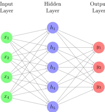
The building block of neural networks is simply a unit or neuron which takes a set of input values, multiplies these inputs by some weights, adds a bias term and applies some non-linear function to the output. These neurons are generally arranged in layers, with each neuron taking as input the output of the neurons in the previous layer. A simple model of a neural network with an input dimension of 4 is shown in Figure 2-1.

The neuron labeled ℎ1, can be computed as follows, where 𝑓 is some non-linear

function:

(16)

𝑥1 𝑥2 𝑥3 𝑥4 Input Layer ℎ1 ℎ2 ℎ3 ℎ4 ℎ5 Hidden Layer 𝑦1 𝑦2 𝑦3 Output Layer

Figure 2-1: Simple Neural Network

One common choice for the function 𝑓 is the rectifier activation function, or simply the function:

𝑓 = 𝑚𝑎𝑥(𝑥, 0)

The choice of architecture, including number of layers, units per layer, and ac-tivation functions is made prior to training, and training of the weights and biases of the network can be performed using back-propagation. This idea simply involves computing the gradient of some loss function of the network output with respect to each parameter and updating each parameter in this direction using gradient descent. In recent years, increased computing power has allowed us to train deeper and deeper neural networks (with increased numbers of layers), which have demonstrated exceptional performance on a variety of tasks.

2.2 Convolutional Neural Networks

Convolutional neural networks are a particular form of neural networks often used for images. These networks are characterized by a specific layer known as a convolutional

(17)

layer, which involves sharing weights between neurons in a layer, and having each unit only connect to a small local patch of the neurons in the previous layer. Figure 2-2 depicts an example 1D convolutional layer, where the same weights are shared between the units of the first layer for each pair of two consecutive inputs. Stride defines the shift between consecutive patches applying the convolution, in this case, the stride is simply 1.

𝑥1 𝑥2 𝑥3 𝑥4 𝑥5 Input Layer ℎ1 ℎ2 ℎ3 ℎ4 Convolution Layer 𝑊1 𝑊1 𝑊1 𝑊1 𝑊2 𝑊2 𝑊2 𝑊2

Figure 2-2: 1D Convolutional Neural Network

In image classification, 2D convolutions of small size, such as 3 × 3 or 5 × 5, are often used [4]. The intuition of such layers is that they serve to provide translational invariance in the identification of particular patterns or features in images, since the same set of weights is applied to each contiguous patch in the image.

Convolutional layers are often followed by max pooling layers, which take the maximum of local regions in the preceding layer, defined by the pooling size and stride. Intuitively, these layers group the results of the convolution, identifying if the target feature exists anywhere within a larger spatial area.

The inclusion of multiple convolutional layers first allows the identification of small local patterns, such as edges or curves, and stacking further convolutional layers allows identification of more complex patterns and shapes, building upon the features

(18)

extracted by preceding layer.

The field of computer vision has been revolutionized by convolutional neural net-works and the substantial jumps in accuracy they have allowed in tasks such as image classification [4]. In recent years, a multitude of different architectures for convolu-tional neural networks have been proposed, leading to increases in accuracies for different tasks and data sets.

In this work we will focus on analyzing and comparing four particular architec-tures: VGG, DenseNet, ResNet, and ResNeXt, which have been proposed in recent years, obtaining state-of-the-art accuracies in image classification tasks.

2.2.1 VGG

The VGG convolutional neural network architecture was introduced by Simonyan et al. based on the idea of very deep convolutional networks [10]. As compared to previous architectures, VGG demonstrated the power of having many stacked convolutional layers, each with a small filter size of 3 × 3. VGG-16 consists of a total of 16 weight layers, divided into 5 blocks, each containing 2 or 3 convolutional layers followed by max pooling, followed by a few fully connected layers.

2.2.2 DenseNet

The key innovation of the DenseNet architecture is the idea of a dense block, in which layer outputs are not simply connected to the next layer, but also to all subsequent layers in the dense block [2]. This modification serves to mitigate the issue of vanishing gradients, which occurs in very deep neural networks, as the gradient often shrinks exponentially as a result of multiplying the gradient with respect to each preceding layer in backpropagation. By adding shorter paths from earlier layers towards the end of the network, the vanishing gradient issue is mitigated, making training more feasible. The DenseNet architecture consists of multiple dense blocks, each containing multiple convolutional layers, with the input to each being the concatenation of the outputs of the previous ones. Dense blocks are separated by a standard convolutional

(19)

and max pooling layer.

2.2.3 ResNet

Residual networks propose an alternative approach to tackling the vanishing gradient issue when training deeper neural networks [1]. Each residual block (composed of multiple layers) adds the input of the block to the output of the final layer of the block to obtain the final output, as shown in Figure 2-3.

Figure 2-3: Residual Network Block Conv 3 × 3 Conv 3 × 3 +

𝐼𝑛𝑝𝑢𝑡 𝑂𝑢𝑡𝑝𝑢𝑡

This can be alternatively interpreted as the network block learning a residual function 𝐹 (𝑥) − 𝑥 rather than the full function 𝐹 (𝑥). These "skip connections" connecting the input of the block to the the output layer again serves to create shorter paths from earlier to later layers, reducing the impact of vanishing gradients. Residual networks are comprised of residual blocks, each with two convolutional layers. The ResNet architecture used in this experiment includes 17 residual blocks, followed by average pooling and a fully connected layer.

2.2.4 ResNeXt

The ResNeXt architecture builds upon the idea of residual networks and introduces the idea of aggregated residual transforms [13]. Each block in ResNeXt consists of multiple separate paths, each consisting of convolution layers. The outputs of each of the separate paths are summed at the end of the block, and the input is also added to this sum, following the pattern described for a residual network. An additional parameter, cardinality, defines the number of separate paths in the ResNeXt block.

The ResNeXt network architecture used includes 17 ResNeXt blocks with cardi-nality 4, followed by average pooling and a fully connected layer.

(20)

2.3 Adversarial Examples

Adversarial examples are a key security concern for machine learning models, par-ticularly for convolutional neural networks. The underlying idea is that a correctly classified image can be transformed slightly such that the object does not change sub-stantially to a human observer, but the network incorrectly classifies the perturbed image.

One common way of generating adversarial examples is by applying multiple it-erations of the Fast Gradient Sign Method (FGSM), which is effectively applying projected gradient descent, identifying a valid perturbation that maximizes the loss of the image [7].

Let 𝑆 denote the space of valid perturbation (e.g. an 𝑙2 ball or bounded 𝑙∞

space). Let 𝐿(𝑥, 𝑦, 𝜃) denote the loss function, 𝑥 denote the natural example, and 𝑥𝑡

an adversarial example at the 𝑡𝑡ℎ _{iteration. Formally, one iteration of FGSM can be}

represented as:

𝑥𝑡+1 =∏︁

𝑥+𝑆

(𝑥𝑡+ 𝛼𝑠𝑔𝑛(∇𝑥𝐿(𝑥, 𝑦, 𝜃)))

2.3.1 Transferability of Adversarial Examples

Prior work has shown that adversarial examples transfer substantially between mod-els; identifying adversarial examples to one model often also serve as adversarial ex-amples to other models. It has been observed that adversarial exex-amples span a large subspace with a substantial overlap between models, likely since decision boundaries of different models are often close in arbitrary directions [11].

The possibility of transferring adversarial examples between models encourages further research into the similarity between the learned representations of different neural network models and how this relates to the phenomenon of transferability.

2.3.2 Adversarial Training

Training networks to be robust to adversarial examples has been a key research ques-tion since the identificaques-tion of adversarial examples. Madry et al. propose the

(21)

fol-lowing saddle point formulation to formally define the objective of training on a data distribution 𝐷 with robustness to a particular class of adversarial perturbations 𝑆 [7]:

min

𝜃 𝜌(𝜃) where 𝜌(𝜃) = E(𝑥,𝑦)∼𝐷[max𝛿∈𝑆 𝐿(𝜃, 𝑥 + 𝛿, 𝑦)]

The empirical minimization can be achieved by performing normal stochastic gra-dient descent for training (outer minimization) and using adversarial examples for training which are identified using projected gradient descent (PGD) as described above. We refer to this procedure as robust or adversarial training. Madry et al. demonstrate that this procedure successfully minimizes the adversarial loss on the training set, and leads to substantial improvements in validation robustness [7].

(22)

(23)

Chapter 3 Related Work

We begin by surveying prior work which focused on understanding the learned repre-sentations of deep convolutional neural networks and how these reprerepre-sentations differ between architectures.

We focus on prior work in three directions, analyzing representation geometry, saliency maps, and convergent learning.

3.1 Representation Geometry

Lu et al. consider and test the hypothesis that the activations of corresponding layers in neural networks, with the same architecture but different initialization, have similar geometries [6]. Particularly, they perform experiments to determine whether the activations of a particular layer can be represented by points in a shared space, and the activations of each network can be an orthogonal transform of the points in this shared space.

To accomplish this, the idea of a shared response model is defined, which allows alignment of the activations from the different neural networks. Each networks’ ac-tivation pattern for a specific layer is defined as 𝑋𝑖 for network 𝑖, which is an 𝑚 × 𝑛

matrix, where 𝑛 is the number of examples, and 𝑚 is the number of units in the layer. The shared space representation 𝑆 is of dimension 𝑘 × 𝑛 and orthogonal transforms

(24)

for each network are defined as 𝑊𝑖. The objective can be formally defined as: min 𝑊𝑖,𝑆 ∑︁ 𝑖 ||𝑋𝑖− 𝑊𝑖𝑆||2𝐹 s.t. (𝑊𝑖)𝑇𝑊𝑖 = 𝐼𝑘

Applying this model to simple convolutional networks and ResNets for both CI-FAR10 and CICI-FAR100, Lu et al. find that a majority of the variance can be explained by the shared representation, particularly for the last hidden layer of a standard con-volutional network, where about 91% of the variance is explained for CIFAR10 and 89% for CIFAR100.

3.2 Convergent Learning

Li et al. study whether networks exhibit convergent learning, which occurs when different networks learn similar sets of features [5]. In order to study this phenomenon, the hypothesis that networks trained with different initializations end up learning the same features in each layer, which may simply be permuted. To identify the optimal matching, the correlation of each pair of features is computed and the optimal matching to optimize the sum of the correlations is identified using the Hopcroft-Karp Algorithm.

The results when applied to AlexNet, with 5 convolutional layers, exhibited that the top matches were highly correlated, while others were almost completely uncorre-lated, suggesting that some of the features are shared, while others are model-specific. Earlier convolutional layers have a large fraction of neurons matched with correlation > 0.5, while later layers have substantially fewer, with only 8% for the fourth convo-lutional layer.

Li et al. also consider the possibility that the features may be linear combinations of each other (one-to-many mapping) rather than simply a one-to-one mapping. By performing Lasso regression with varying regularization parameter, they identify that sparse coefficients are strongly predictive for the first two convolutional layers, with an average of 2.5 mapped features, suggesting that small groups of features in the

(25)

two networks span similar subspaces. For later convolutional layers, the regression did not fit well, suggesting that the learned features are not substantially correlated.

3.3 Model Visualizations and Saliency Maps

Rather than particularly focusing on comparing the representations of different net-works, work related to saliency maps focuses on understanding and visualizing the way that networks learn, specifically what parts or features of an image lead to the output of a particular class. Simonyan et al. approach this task in two ways, first by identifying an image that maximizes the score of a particular class, and second by identifying the significance of each input pixel on any class score [9].

Let 𝑆𝐶(𝑥) denote the logit (value prior to softmax) corresponding to class 𝐶 for

input image 𝑥, and let 𝜆 be a regularization parameter.

The first task can be formalized as follows. The desired "class image" can be identified as:

arg max

𝑥

𝑆𝐶(𝑥) − 𝜆||𝑥||22

A local maxima can be identified by simply performing gradient descent / back-propagation with fixed weights, simply updating 𝑖 at each iteration.

The second task can be formalized by considering the first-order Taylor expansion of 𝑆𝐶(𝑥).

𝑆𝐶(𝑥) ≈ 𝑤𝑇𝑥 + 𝑏

For a given image 𝑥0, 𝑤 is simply the derivative of 𝑆𝐶 with respect to 𝑥 at 𝑥0 or:

𝑤 = 𝜕𝑆𝐶 𝜕𝑥 |𝑥0

For color images, the max weight for a pixel over the color channels can be considered to generate a saliency map.

(26)

(27)

Chapter 4 Experiment Design

In this work, we focus on analyzing similarity of image classification networks based on two main approaches: comparing geometries of the final hidden representations and comparing saliency maps. In Section 4.1, we describe the the experiments related to hidden representation comparison, including the transformation and cluster analysis experiments. In Section 4.2, we describe the experiment related to saliency maps.

4.1 Hidden Representation Comparison

The dimensionality of this final hidden representation differs between network archi-tectures, ranging from 100 to 2000 dimensions in common neural network architec-tures utilized for classification.

We choose to focus on comparing this particular representation for multiple rea-sons. First, any classification neural network can be understood intuitively as first converting an input (image) to an embedding in a high dimensional space, and then applying a linear classifier in this space. The final hidden representation is this high dimensional space, and the last layer of the network applies a linear classifier to the representations. The linear separability provides motivation to interpret these representations geometrically, and particularly consider how the geometries of these embeddings differ based on the choice of network architecture.

(28)

particular is the effectiveness of transfer learning. In transfer learning, the last hidden representation of a pre-trained network (e.g. based on ImageNet) is used as the input features for training on a different classification task. This suggests that the final hidden representation encodes substantial semantic information regarding the original image, beyond simply the class information of the original classification task.

The fundamental hypothesis tested in these experiments is that there exists similar geometries between the hidden representations of different neural networks trained to perform the same classification task.

4.1.1 Transformation Experiments

In these experiments, we explore if there exist either orthogonal or linear transforma-tions between the hidden representatransforma-tions of different neural networks.

We will begin by giving particular details on the process of identifying linear and orthogonal transformation between two matrices. We will then describe the overall experiment procedure using the ideas of these transformations. Each of the experiments conducted focuses on comparing a pair of networks, trained with the same training data, and which may be of the same or different architectures.

Linear Transformation

To explore if two matrices 𝐴 and 𝐵 are represented well by a linear transformation, we would like to identify 𝑋 such that 𝐴𝑋 is as close to 𝐵 as possible. Choosing a squared error penalty, this is equivalent to optimizing:

min

𝑋 ||𝐴𝑋 − 𝐵||𝐹

We note that this is simply performing multivariate linear regression independently on each column of 𝐵 with features equal to the columns of matrix 𝐴, with the coefficients of each regression providing a column of 𝑋.

(29)

Orthogonal Transformation

We would also like to explore whether 𝐴 and 𝐵 are related by an orthogonal transfor-mation, or in geometric terms, by a rotation or reflection (preserving distance between points). Now, we would like to identify 𝑋 such that 𝐴𝑋 is as close to 𝐵 as possible, with the additional constraint that 𝑋 is an orthogonal matrix, rather than an arbi-trary linear map. Note that if 𝐴 and 𝐵 are not of the same dimension, we can add columns of zeros to the smaller matrix to ensure that 𝑋 is a square matrix. Again, with a squared error penalty, this is equivalent to optimizing:

min

𝑋 ||𝐴𝑋 − 𝐵||𝐹 𝑠.𝑡. 𝑋 𝑇

𝑋 = 𝐼

This is simply the objective of the Orthogonal Procrustes problem, and the optimal ˆ

𝑋 can be expressed based on the SVD of the matrix 𝐵𝐴𝑇 [8]. 𝐵𝐴𝑇 = 𝑈 Σ𝑉𝑇

ˆ

𝑋 = 𝑈 𝑉𝑇

Note that for any orthogonal matrix 𝑋, 𝐴 = 𝑋𝐵 implies that ||𝐴||𝐹 = ||𝐵||𝐹. In order

to also allow for scale transforms (different Frobenius norms for both representations), we identify 𝑋 using 𝐴

||𝐴||𝐹 and

𝐵

||𝐵||𝐹, which serves to normalize both matrices by their

Frobenius norms prior to identifying the optimal orthogonal transform. Experiment Structure

Let 𝑓1 denote the function mapping input images to the final hidden representation

of network 1, and let 𝑓2 denote the function mapping input images to the final hidden

representation of network 2. We will also assume that each dataset is divided into partitions 𝑋𝑡𝑟𝑎𝑖𝑛_{, 𝑋}𝑣𝑎𝑙_{, and 𝑋}𝑡𝑒𝑠𝑡_.

We can describe the experiment overview as follows:

(30)

training parameters are described in Chapter 5. 2. Evaluate 𝐻𝑣𝑎𝑙

1 = 𝑓1(𝑋𝑣𝑎𝑙), 𝐻2𝑣𝑎𝑙 = 𝑓2(𝑋𝑣𝑎𝑙), 𝐻1𝑡𝑒𝑠𝑡 = 𝑓1(𝑋𝑡𝑒𝑠𝑡), and 𝐻2𝑡𝑒𝑠𝑡 =

𝑓2(𝑋𝑡𝑒𝑠𝑡)

3. Center each matrix at the origin by subtracting the mean row from each matrix, with resulting matrices ¯𝐻𝑣𝑎𝑙

1 , ¯𝐻2𝑣𝑎𝑙, ¯𝐻1𝑡𝑒𝑠𝑡, ¯𝐻2𝑡𝑒𝑠𝑡.

4. Find optimal linear / orthogonal transformation 𝑋 mapping ¯𝐻𝑣𝑎𝑙

1 to ¯𝐻2𝑣𝑎𝑙. Note

that as described in Section 4.1.2, for an orthogonal transformation, we identify the transformation between 𝐻¯𝑣𝑎𝑙

1 || ¯𝐻𝑣𝑎𝑙 1 ||𝐹 and ¯ 𝐻𝑣𝑎𝑙 2 || ¯𝐻𝑣𝑎𝑙 2 ||𝐹. 5. Compute ˆ𝐻𝑡𝑒𝑠𝑡

2 as follows: For linear transformation:

ˆ

𝐻₂𝑡𝑒𝑠𝑡 = 𝑋 ¯𝐻₁𝑡𝑒𝑠𝑡 For orthogonal transformation:

ˆ 𝐻₂𝑡𝑒𝑠𝑡= 𝑋 ¯𝐻₁𝑡𝑒𝑠𝑡||𝐻 𝑡𝑒𝑠𝑡 2 ||𝐹 ||𝐻𝑡𝑒𝑠𝑡 1 ||𝐹

6. Ratio of unexplained variance can be calculated as follows: Variance Unexplained = || ˆ𝐻2𝑡𝑒𝑠𝑡− ¯𝐻2𝑡𝑒𝑠𝑡||2𝐹

|| ¯𝐻𝑡𝑒𝑠𝑡 2 ||2𝐹

To better understand the shared geometries of the two networks, we will use the linear classifier learned by network 2, which we will refer to as 𝐶2, to separate the

space of the hidden representation into two subspaces. One subspace corresponds to that spanned by the vectors corresponding to the directions for each of the classes (columns of 𝐶2), while the other is simply the complement of this space, or the

null-space of 𝐶2. This separation allows us to separate the variance unexplained within

the space of the linear classifier (corresponding to class predictions) from that of the null-space (irrelevant to class predictions) and analyze them independently.

(31)

Let 𝑅𝐶2 denote a matrix with columns forming an orthonormal basis of the row

space of 𝐶2, and 𝑁𝐶2 as the matrix with columns forming an orthonormal basis of

the null-space. Using these definitions, we can consider the unexplained variance by taking the projection onto the particular subspace. The variance unexplained in the space of the linear classifier can be defined as:

Classifier Space Unexplained Variance = || ˆ𝐻2𝑡𝑒𝑠𝑡𝑅𝐶2− ¯𝐻2𝑡𝑒𝑠𝑡𝑅𝐶2||2𝐹

|| ¯𝐻𝑡𝑒𝑠𝑡 2 𝑅𝐶2||2𝐹

Similarly, the unexplained variance in null-space of the linear classifier can be defined as:

Classifier Null-Space Unexplained Variance = || ˆ𝐻2𝑡𝑒𝑠𝑡𝑁𝐶2− ¯𝐻2𝑡𝑒𝑠𝑡𝑁𝐶2||2𝐹

|| ¯𝐻𝑡𝑒𝑠𝑡 2 𝑁𝐶2||2_𝐹

4.1.2 Cluster Analysis Experiments

In this experiment, we analyze the relative positioning of clusters corresponding to classes in the hidden representation space and consider the similarities between dif-ferent architectures. The experiment structure is as follows:

1. Take the validation set 𝑋𝑣𝑎𝑙 and divide it into 𝐶 partitions, 𝑋𝑣𝑎𝑙

1 , 𝑋2𝑣𝑎𝑙, ...𝑋𝐶𝑣𝑎𝑙,

corresponding to the class label, where 𝐶 is the number of classes. 2. For each pair of classes 𝑖, 𝑗, with 𝑖 ̸= 𝑗:

∙ Compute the average pairwise distance between each point in 𝑓1(𝑋𝑖𝑣𝑎𝑙)and

𝑓1(𝑋𝑗𝑣𝑎𝑙), and let this distance be 𝑑 𝑖𝑗 1.

∙ Similarly compute the average pairwise distance between each point in 𝑓2(𝑋𝑖𝑣𝑎𝑙) and 𝑓2(𝑋𝑗𝑣𝑎𝑙), and let this distance be 𝑑

𝑖𝑗 2.

3. Construct vectors 𝑑1 and 𝑑2 by concatenating the average class distances for all

pairs of classes, each vector of length (︀𝐶 2

)︀ .

4. Compute the correlation coefficient between 𝑑1 and 𝑑2, which measures the

(32)

We can perform the experiment described above with different distance metrics, in-cluding 𝐿1, 𝐿2 and cos distances.

For pairs of networks with very similar relative positioning of clusters (including scaling), we expect to observe correlations close to 1, while with different relative positioning of clusters, we expect substantially lower correlations.

4.2 Saliency Comparison Experiments

The goal of these experiments is to understand more broadly whether different net-works identify an image in the same way, by focusing on similar parts or features of an image.

The basis of this experiment is the work by Simonyan et al. developing saliency maps, described in Section 3.3. The importance of a pixel to a final classification can be estimated by the gradient of the class-output with respect to the input pixel, forming a saliency map.

The saliency maps are compared using the following procedure. The absolute value is considered when comparing saliency maps in order to simply focus on significance of a pixel, regardless of positive or negative effect on output classification.

1. Compute saliency map for the same input on two networks.

2. Take the absolute value and normalize to the range 0-1 (with 99𝑡ℎ _percentile

taking value 1 to account for outliers).

3. Compute mean squared error between the normalized saliency maps.

4. Apply Gaussian blurs to both saliency maps with 𝜎 = 1 and 𝜎 = 2 and compute corresponding mean square error between the blurred saliency maps.

Blurring the saliency maps allows mitigation of local variance, where one map may focus more on neighboring pixels to those of the other map. The computed mean squared errors are averaged over the images of the test set to compute an average error metric for any two networks.

(33)

Chapter 5 Experimental Results

To evaluate the experiments described in Chapter 4, we perform the experiments on multiple real-world image classification datasets.

We will begin by giving short descriptions of the datasets, architectures and train-ing parameters utilized in the experiments, and then describe the particular results obtained from each experiment.

5.1 Experiment Details

Datasets

The experiments were conducted on the CIFAR10, CIFAR100, and SVHN datasets. In order to accommodate separate training and validation sets, 20% of the standard training set was separated as a validation set.

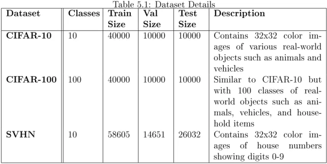
Table 5.1 summarizes the key facts of the chosen datasets.

In addition to the three datasets with the given labels, we also make additional tests using the CIFAR-10 dataset with random labels. This serves to compare the behavior of neural networks trained on a generalizable task, versus one of memoriza-tion.

(34)

Table 5.1: Dataset Details Dataset Classes Train

Size ValSize TestSize Description

CIFAR-10 10 40000 10000 10000 Contains 32x32 color im-ages of various real-world objects such as animals and vehicles

CIFAR-100 100 40000 10000 10000 Similar to CIFAR-10 but with 100 classes of real-world objects such as ani-mals, vehicles, and house-hold items

SVHN 10 58605 14651 26032 Contains 32x32 color im-ages of house numbers showing digits 0-9

Architectures

The architectures tested in these experiments include VGG-16, ResNet50, DenseNet, and ResNeXt29_4x64d. The number of parameters of each model is shown in the table below.

Model Details

Model Number of

pa-rameters VGG-16 14,728,266 ResNet 23,520,842 DenseNet 1,000,618 ResNeXt 27,104,586 Training Procedures

Each neural network was trained on the training data using data augmentation, in-cluding random crops, first padding each dimension by 4 units, and horizontal flips. Each network was trained using SGD with Nesterov momentum, with learning rate = 0.1, momentum = 0.9 and weight decay = 0.0005. Networks on CIFAR-10 and

(35)

CIFAR-100 were trained for 300 epochs, robust networks on CIFAR-10 were trained for 100 epochs, and networks for SVHN were trained for 80 epochs.

5.2 Results

5.2.1 Transformation Results

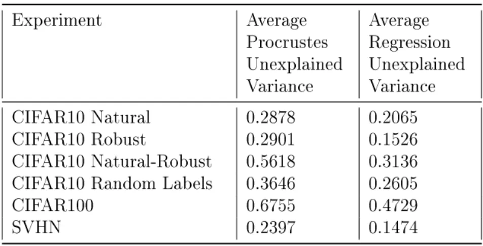
Table 5.2: Transformation Average Results

Experiment Average Procrustes Unexplained Variance Average Regression Unexplained Variance CIFAR10 Natural 0.2878 0.2065 CIFAR10 Robust 0.2901 0.1526 CIFAR10 Natural-Robust 0.5618 0.3136 CIFAR10 Random Labels 0.3646 0.2605

CIFAR100 0.6755 0.4729

SVHN 0.2397 0.1474

The transformation experiment results demonstrate that hidden representations of different networks trained on the same task show substantial similarity. As shown in Table 5.2, networks trained for classifying CIFAR10 and SVHN on average had a ratio of unexplained variance < 0.3 by simply applying an orthogonal transformation (Procrustes), but networks trained on CIFAR100 appear to be more substantially different, with average Procrustes unexplained variance of 0.6755.

The transformation data also provides some insights into the differences between natural and adversarially trained networks. The average unexplained variances be-tween networks trained traditionally or networks trained adversarially for CIFAR10 are both < 0.3, while the average Procrustes unexplained variance between a naturally trained and adversarially trained network is 0.5618, suggesting that the geometry of the hidden representation of adversarially trained networks is substantially different than that of naturally trained ones.

(36)

The tests with random labels on CIFAR-10 serves to quantify differences between a network trained on a generalizable task as opposed to one that simply memorizes an aribtrary input distribution. It is evident that both the average Procrustes and regression unexplained variances are higher for random labels than natural training, which as intuitively expected, suggests that the hidden layer geometry is less consis-tent when training on a task that requires memorization.

One hypothesis related to the similarity of the hidden representation is that the hidden representation primarily encodes the class information, and the similarity between different networks is caused solely by similarity between class predictions. We can evaluate the similarity of features not utilized in class output by looking at the null-space unexplained variance, as described in Section 4.1.1. As the results in Tables A.1-6 show, the null-space unexplained variance ratio is substantially higher than that of the overall unexplained variance, but many network pairs have null-space unexplained variance ratios substantially less than 1, suggesting that even features not used for classification are similar across networks.

Another key insight from the results is the observed variations of unexplained variance between different model architectures. Particularly, when comparing two ResNext networks (with different initializations), the unexplained variance is sub-stantially lower than any other pair of networks. This result is consistent over all the datasets, including CIFAR10, CIFAR100, and SVHN, which suggests that the consistency of ResNeXt models is a phenomenon related to the architecture and not dependent on the dataset or initialization. Similarly, it appears that ResNet and ResNeXt models are more similar than other pairs of different networks, suggesting that networks with similar structures (e.g. residual connections) lead to more similar hidden representations.

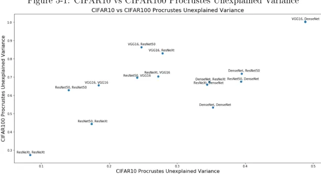
More generally, the trends observed of unexplained variance between different pairs of architectures appears correlated between the different datasets. In Figure 5-1, it is evident that a positive correlation exists between the Procrustes unexplained variance for a pair of networks on the CIFAR10 and CIFAR100 datasets, suggesting that the similarities are related to the network structures as opposed to dataset effects

(37)

Figure 5-1: CIFAR10 vs CIFAR100 Procrustes Unexplained Variance

or randomness. Particularly, it is evident that (ResNeXt, ResNeXt) is the most similar pair of architectures (least unexplained variance) for both datasets, while (VGG16, DenseNet) is the least similar pair of architectures for both datasets (most unexplained variance). A similar correlation is evident when comparing CIFAR10 and SVHN Procrustes Unexplained Variance (Figure B-1).

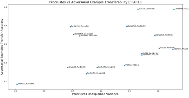
Another connection evident from the transformation experiment results is similar-ity between Procrustes unexplained variance and adversarial example transferabilsimilar-ity, quantified as the accuracy of adversarial examples constructed on the first model and evaluated on the second. In Tables A.1 and A.2, it is evident that the pair of ResNeXt models also consistently has the lowest adversarial example accuracy, with about 90% of adversarial examples transferring between the models for CIFAR10. In Figure 5-2, we observe that a positive correlation exists between Procrustes unexplained variance and adversarial example transfer accuracy for CIFAR10. This correlation suggests that pairs of models with more similar hidden representation geometries may be more susceptible to adversarial example transfer attacks. A similar correlation is also evident for CIFAR100, shown in Figure B-2.

(38)

Figure 5-2: CIFAR10 Adversarial Example Transferability

results from shared non-robust features, which are highly predictive features but sensitive to small perturbations [3]. Based on this perspective, our results demonstrate that networks which learn similar non-robust features also have more similar hidden representations, suggesting that the hidden representation may serve as an encoding of the particular non-robust features used.

5.2.2 Cluster Analysis Results

Table 5.3: Transformation Average Results

Experiment Average L1

Correlation Average L2Correlation Average cosCorrelation

CIFAR10 Natural 0.7259 0.8461 0.8343

CIFAR10 Robust 0.9359 0.9259 0.9354

CIFAR10 Natural-Robust 0.6668 0.7508 0.8128 CIFAR10 Random Labels 0.2450 0.1579 0.1639

CIFAR100 0.6255 0.5978 0.7651

(39)

The average correlations shown in Table 5.3 suggest that the relative positioning of clusters exhibit substantial similarity when compared between pairs of networks. Particularly, adversarially trained / robust networks show substantially more similar-ity than natural networks, suggesting that the adversarial training procedure leads to a more consistent relative cluster positioning than natural training.

Training with random labels appears to have inconsistent cluster positioning, with very low average correlation, and many network pairs exhibiting correlations around 0.

Comparing the correlations between particular model pairs in Tables A.7-9, it is evident that the pair of ResNeXt models consistently exhibits the highest correlation for all datasets and distance measures. Particularly, ResNeXt models are also similar for the random labels experiment, exhibiting correlation above 0.75. The similarity of ResNeXt models parallels the observations from the transformation experiments, in which ResNeXt models also exhibited the lowest unexplained variance.

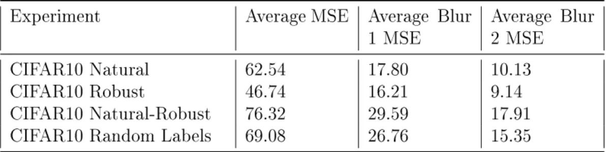
5.2.3 Saliency Comparison Results

Table 5.4: Saliency Average Results Experiment Average MSE Average Blur

1 MSE Average Blur2 MSE

CIFAR10 Natural 62.54 17.80 10.13

CIFAR10 Robust 46.74 16.21 9.14

CIFAR10 Natural-Robust 76.32 29.59 17.91 CIFAR10 Random Labels 69.08 26.76 15.35

From the saliency comparisons, it is evident that the saliency maps of robust net-works are substantially different from those of natural netnet-works, with mean squared errors substantially larger than those of pairs of natural or robust networks. For training with random labels, the saliency maps also exhibit higher MSE than natural or robust networks for all blur levels, but still lower than the errors between natural and robust networks. Intuitively, the features memorized by the networks trained

(40)

with random labels are less consistent between networks as opposed to generalizable features.

The difference between the MSE for pairs of naturally trained and pairs of ad-versarially trained networks is large when directly comparing the saliencies, but the difference is substantially reduced when comparing blurred saliency maps. The lower MSE for pairs of adversarially trained networks suggests that they generally identify more consistent features as opposed to naturally trained networks. These differences also suggest that different naturally trained networks likely identify features in similar regions but focus on different pixels, but when blurred, the maps are substantially more similar and comparable to pairs of robust networks. This result parallels the phenomena observed by Tsipras et al, that robust features are generally less noisy [12].

When comparing the saliency maps of particular pairs of network architectures, it is evident that pairs of ResNeXt networks, ResNet networks, and ResNeXt and ResNet pairs have the most similar saliency maps. This parallels the similarities observed in the transformation and cluster analysis experiments, and similarity in hidden layer geometry is likely paralleled by similarity in identified features in input.

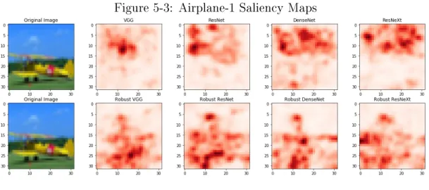
Figure 5-3: Airplane-1 Saliency Maps

From a qualititative analysis of the saliency maps generated for each network (Figures 5-3,B.1-10), clear differences are visible between those of robust networks and natural networks, again corroborating observations by Tspiras et al. of robust

(41)

features [12]. Particularly, for images of planes and ships in CIFAR10, it is evident that natural networks appear to focus more on background features such as the sky or water, while robust networks focus more on the particular foreground object.

(42)

(43)

Chapter 6 Conclusion

In this work, we explored multiple ways of comparing the learned representations of neural networks including using orthogonal and linear transformations of hidden representations, analyzing distances between clusters, and comparing saliency maps based on input gradients.

These experiments were applied to a variety of convolutional neural network ar-chitectures including both naturally trained and adversarially trained networks. We found that substantial differences exist in the hidden representation geometries of naturally trained and adversarial trained models, as well as in the saliency maps be-tween these different types of networks. Further work analyzing the differences in the geometries of these representations may provide clues into understanding the funda-mental differences between robust and non-robust networks and also provide insights into improved training of robust models.

One of our key findings is that there exists a correlation between hidden represen-tation similarity and adversarial example transferability. Models with more similar hidden representations also appear to generally have higher degrees of adversarial example transferability. Based on recent work defining adversarial examples in terms of non-robust features, this correlation demonstrates that networks relying on more similar non-robust features also have similar hidden representations, which suggests that the hidden representation may encode information regarding the features used by a network. Understanding this phenomenon further may be useful to train networks

(44)

to utilize different non-robust features, which can serve as a defense against transfer attacks.

Another key insight from these experiments is that certain network architectures consistently learn more similar representations than others. Particularly, all the ex-periments show that ResNeXt models, trained from different random initializations, tend to learn very similar hidden representations, identify more similar features in in-put images, and have very high adversarial example transferability. This consistency particularly holds true for the ResNeXt architecture, but not for other architectures. This property may be desirable in certain use-cases where consistency is preferred, or particularly undesirable in avoiding adversarial example transferability. A key open question is why ResNeXt models end up learning such similar representations and whether it is a direct result of the architecture design, particularly the grouped convolution structure.

Overall, this work makes progress on understanding the differences between net-works by comparing the final learned hidden representations and salient input features of different networks. The results of this work provide insight into different cases and architectures where networks learn in more similar and different ways, which relates to the fundamental question of understanding how deep neural networks learn and has applications to improving the security of neural networks to adversarial examples.

(45)

Appendix A

Tables

(46)

Table A.1: CIFAR10 Alignment Results

From Model To Model UnexplainedProcrustes Variance Regression Unexplained Variance Procrustes Null-Space Unexplained Variance Regression Null-Space Unexplained Variance Adversarial Examples Accuracy VGG16 VGG16 0.184270 0.146789 0.666918 0.482900 0.4828 VGG16 ResNet50 0.247618 0.191796 0.893924 0.547736 0.5412 ResNet50 VGG16 0.240935 0.192976 0.773964 0.562538 0.5438 VGG16 DenseNet 0.488386 0.346081 0.900929 0.751790 0.5299 DenseNet VGG16 0.488302 0.300590 2.082736 0.583522 0.6561 VGG16 ResNeXt 0.278264 0.198325 1.074087 0.650768 0.6045 ResNeXt VGG16 0.272064 0.220282 0.861548 0.556557 0.6527 ResNet50 ResNet50 0.140486 0.130486 0.437159 0.357438 0.3478 ResNet50 DenseNet 0.393721 0.277497 0.752290 0.582334 0.2924 DenseNet ResNet50 0.395015 0.243905 1.958604 0.551556 0.4904 ResNet50 ResNeXt 0.174053 0.135159 0.603086 0.426631 0.3861 ResNeXt ResNet50 0.174023 0.167599 0.619259 0.425409 0.2833 DenseNet DenseNet 0.352521 0.237106 0.908766 0.531064 0.3036 DenseNet ResNeXt 0.346962 0.209725 1.932825 0.513107 0.5887 ResNeXt DenseNet 0.344163 0.228878 0.693538 0.474404 0.3254 ResNeXt ResNeXt 0.083972 0.077577 0.326857 0.257091 0.1045

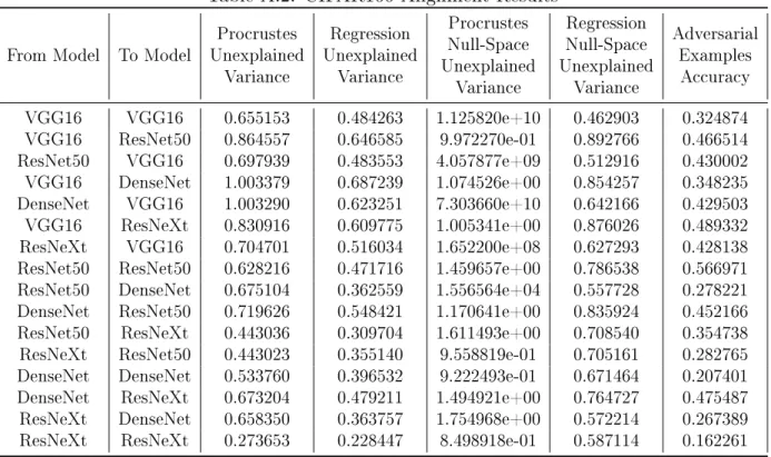
Table A.2: CIFAR100 Alignment Results

From Model To Model UnexplainedProcrustes Variance Regression Unexplained Variance Procrustes Null-Space Unexplained Variance Regression Null-Space Unexplained Variance Adversarial Examples Accuracy VGG16 VGG16 0.655153 0.484263 1.125820e+10 0.462903 0.324874 VGG16 ResNet50 0.864557 0.646585 9.972270e-01 0.892766 0.466514 ResNet50 VGG16 0.697939 0.483553 4.057877e+09 0.512916 0.430002 VGG16 DenseNet 1.003379 0.687239 1.074526e+00 0.854257 0.348235 DenseNet VGG16 1.003290 0.623251 7.303660e+10 0.642166 0.429503 VGG16 ResNeXt 0.830916 0.609775 1.005341e+00 0.876026 0.489332 ResNeXt VGG16 0.704701 0.516034 1.652200e+08 0.627293 0.428138

ResNet50 ResNet50 0.628216 0.471716 1.459657e+00 0.786538 0.566971

ResNet50 DenseNet 0.675104 0.362559 1.556564e+04 0.557728 0.278221

DenseNet ResNet50 0.719626 0.548421 1.170641e+00 0.835924 0.452166

ResNet50 ResNeXt 0.443036 0.309704 1.611493e+00 0.708540 0.354738

ResNeXt ResNet50 0.443023 0.355140 9.558819e-01 0.705161 0.282765

DenseNet DenseNet 0.533760 0.396532 9.222493e-01 0.671464 0.207401

DenseNet ResNeXt 0.673204 0.479211 1.494921e+00 0.764727 0.475487

ResNeXt DenseNet 0.658350 0.363757 1.754968e+00 0.572214 0.267389

(47)

Table A.3: SVHN Alignment Results

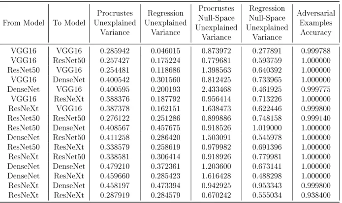
Table A.4: CIFAR10 Random Labels Alignment Results

(48)

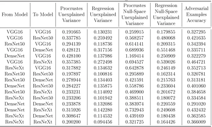
Table A.5: CIFAR10 Robust Alignment Results

(49)

Table A.6: CIFAR10 Natural vs Robust Alignment Results

From Model To Model UnexplainedProcrustes Variance Regression Unexplained Variance Procrustes Null-Space Unexplained Variance Regression Null-Space Unexplained Variance

Robust ResNeXt ResNeXt 0.462933 0.228568 2.246026 0.511147

ResNeXt Robust ResNeXt 0.462950 0.239653 0.463129 0.239875

Robust ResNeXt DenseNet 0.505151 0.318532 1.026233 0.594218

DenseNet Robust ResNeXt 0.518877 0.301458 0.518999 0.301563

Robust DenseNet ResNeXt 0.606759 0.269317 3.639816 0.535449

ResNeXt Robust DenseNet 0.604990 0.230805 0.602381 0.229799

Robust DenseNet DenseNet 0.577942 0.314886 1.536091 0.590250

DenseNet Robust DenseNet 0.577950 0.358365 0.577140 0.358076

Robust ResNeXt ResNet50 0.501325 0.272098 2.254486 0.570917

ResNet50 Robust ResNeXt 0.501368 0.328568 0.501493 0.328466

Robust ResNet50 ResNeXt 0.478018 0.228439 2.569517 0.533353

ResNeXt Robust ResNet50 0.478028 0.221536 0.478034 0.221530

Robust DenseNet ResNet50 0.666138 0.314719 3.592093 0.598998

ResNet50 Robust DenseNet 0.665542 0.352813 0.665767 0.353176

Robust ResNet50 DenseNet 0.527197 0.337334 1.167352 0.648857

DenseNet Robust ResNet50 0.538050 0.313314 0.537821 0.313218

Robust ResNet50 ResNet50 0.517313 0.262093 2.576403 0.557514

ResNet50 Robust ResNet50 0.517370 0.272427 0.516691 0.272128

Robust ResNeXt VGG16 0.570536 0.315027 1.895872 0.638113 VGG16 Robust ResNeXt 0.600195 0.401612 0.599908 0.401267 Robust VGG16 ResNeXt 0.493570 0.304279 2.005055 0.686582 ResNeXt Robust VGG16 0.482937 0.236225 0.486528 0.237789 Robust DenseNet VGG16 0.764251 0.353655 3.656232 0.602837 VGG16 Robust DenseNet 0.764258 0.525140 0.763273 0.524859 Robust VGG16 DenseNet 0.578875 0.393244 1.206101 0.767939 DenseNet Robust VGG16 0.578862 0.322612 0.580106 0.321759 Robust ResNet50 VGG16 0.580319 0.288045 2.220516 0.636582 VGG16 Robust ResNet50 0.619143 0.437371 0.618937 0.436993 Robust VGG16 ResNet50 0.522943 0.316875 1.630994 0.627861 ResNet50 Robust VGG16 0.512842 0.270698 0.515881 0.272860 Robust VGG16 VGG16 0.600786 0.344672 1.766686 0.606427 VGG16 Robust VGG16 0.600779 0.359881 0.597156 0.358819

(50)

Table A.7: CIFAR10 Cluster Analysis Results Model 1 Model 2 Average L1

Correlation AverageCorrelationL2 Average cosCorrelation

VGG16 VGG16 0.470040 0.685574 0.621092 VGG16 ResNet50 0.627994 0.751747 0.789100 VGG16 DenseNet 0.628559 0.677222 0.599716 VGG16 ResNeXt 0.566594 0.701652 0.657978 ResNet50 ResNet50 0.818046 0.944206 0.962606 ResNet50 DenseNet 0.684218 0.884814 0.889330 ResNet50 ResNeXt 0.695679 0.940604 0.965254 DenseNet DenseNet 0.947741 0.956820 0.950888 DenseNet ResNeXt 0.837792 0.932963 0.915298 ResNeXt ResNeXt 0.982343 0.985439 0.991791

Table A.8: CIFAR100 Cluster Analysis Results Model 1 Model 2 Average L1

(51)

Table A.9: SVHN Cluster Analysis Results Model 1 Model 2 Average L1

Table A.10: CIFAR10 Robust Cluster Analysis Results Model 1 Model 2 Average L1

(52)

Table A.11: CIFAR10 Natural vs Robust Cluster Analysis Results Regular

Model RobustModel AverageCorrelationL1 AverageCorrelationL2 Average cosCorrelation VGG16 Robust VGG16 0.422097 0.453349 0.445527 VGG16 Robust ResNet50 0.627754 0.751074 0.716413 ResNet50 Robust VGG16 0.450742 0.754436 0.781730 VGG16 Robust DenseNet 0.404872 0.493622 0.573243 DenseNet Robust VGG16 0.804658 0.791361 0.871749 VGG16 Robust ResNeXt 0.664473 0.636633 0.690677 ResNeXt Robust VGG16 0.811662 0.840803 0.866656 ResNet50 Robust ResNet50 0.495609 0.822618 0.869671 ResNet50 Robust DenseNet 0.510573 0.736578 0.857742 DenseNet Robust ResNet50 0.810093 0.775936 0.907304 ResNet50 Robust ResNeXt 0.499113 0.844922 0.916145 ResNeXt Robust ResNet50 0.837677 0.831941 0.911583 DenseNet Robust DenseNet 0.885623 0.864123 0.945883 DenseNet Robust ResNeXt 0.840701 0.870474 0.916777 ResNeXt Robust DenseNet 0.798961 0.716402 0.849686 ResNeXt Robust ResNeXt 0.804979 0.828978 0.884500

(53)

Table A.12: CIFAR10 Random Cluster Analysis Results Model 1 Model 2 Average L1

VGG16 VGG16 0.145959 0.088148 0.081203 VGG16 ResNet50 0.445316 0.416918 0.326583 VGG16 DenseNet -0.041624 -0.094516 -0.138950 VGG16 ResNeXt 0.107664 0.033150 0.031433 ResNet50 ResNet50 0.419303 0.182690 0.084417 ResNet50 DenseNet 0.338550 0.293678 0.419404 ResNet50 ResNeXt 0.176781 -0.038098 0.112519 DenseNet DenseNet 0.129814 0.034937 0.165999 DenseNet ResNeXt -0.052758 -0.101278 -0.206378 ResNeXt ResNeXt 0.781428 0.763017 0.762442

Table A.13: CIFAR10 Saliency Comparison Results Model 1 Model 2 Average

Saliency MSE Blur 1 MSE Blur 2 MSE VGG16 VGG16 59.705841 15.054407 7.877510 VGG16 ResNet50 67.035361 22.277499 13.758103 VGG16 DenseNet 66.861288 20.651534 11.849692 VGG16 ResNeXt 71.390237 23.909150 14.984485 ResNet50 ResNet50 55.921603 16.853876 9.207124 ResNet50 DenseNet 59.389641 17.366500 9.513009 ResNet50 ResNeXt 64.446829 15.915617 9.054121 DenseNet DenseNet 58.488373 15.009078 7.704466 DenseNet ResNeXt 69.599941 18.098575 10.764805 ResNeXt ResNeXt 52.519565 12.893992 6.573975

(54)

Table A.14: CIFAR10 Robust Saliency Comparison Results From

Model To Model AverageSaliency MSE Blur 1 MSE Blur 2 MSE ResNet50 ResNet50 38.482083 12.096067 6.320665 VGG16 ResNeXt 53.629556 19.701835 12.242177 DenseNet ResNeXt 48.458828 16.412964 9.062714 VGG16 VGG16 43.191582 13.512466 7.065569 ResNet50 DenseNet 47.179763 16.319820 9.179240 VGG16 DenseNet 55.327485 21.409505 12.580958 DenseNet DenseNet 48.887040 17.729133 9.613883 ResNeXt ResNeXt 37.150008 10.861393 5.510408 ResNet50 ResNeXt 43.300087 13.938615 7.376463 VGG16 ResNet50 51.760987 20.109688 12.506219

Table A.15: CIFAR10 Natural vs Robust Saliency Comparison Results Natural

Model RobustModel AverageSaliency MSE Blur 1 MSE Blur 2 MSE ResNet50 DenseNet 75.593292 29.611957 17.290146 DenseNet ResNet50 79.378788 31.973102 19.257739 ResNeXt ResNeXt 76.572945 30.309570 19.229510 ResNeXt ResNeXt 76.146260 28.960086 18.124106 DenseNet DenseNet 78.251298 30.289060 17.099496 DenseNet DenseNet 77.633333 30.742743 17.886858 VGG16 VGG16 72.510371 26.650240 15.765603 VGG16 VGG16 72.241228 26.371156 15.381888 ResNet50 ResNeXt 74.877114 29.121717 17.037190 ResNeXt ResNet50 77.268995 26.680284 16.123939 VGG16 DenseNet 74.751376 28.488151 17.479688 DenseNet VGG16 78.337677 32.134962 18.972509 ResNet50 ResNet50 74.656900 30.204690 17.560210 ResNet50 ResNet50 72.929672 29.761362 18.505630 VGG16 ResNeXt 76.783722 29.564837 19.541914 ResNeXt VGG16 77.344923 31.493661 19.489271 DenseNet ResNeXt 78.474043 31.422308 19.327872 ResNeXt DenseNet 79.837081 25.360078 14.769904 VGG16 ResNet50 74.755212 29.166383 18.892393 ResNet50 VGG16 78.080040 33.469445 20.387284

(55)

Table A.16: CIFAR10 Random Saliency Comparison Results Model 1 Model 2 Average

Saliency MSE Blur 1 MSE Blur 2 MSE ResNeXt ResNeXt 58.714520 17.799665 11.335997 ResNet50 ResNet50 58.200090 16.406695 8.985058 DenseNet DenseNet 65.646425 29.671317 15.206374 ResNet50 DenseNet 74.454096 32.411059 20.160389 VGG16 ResNet50 71.847246 32.373611 17.915761 VGG16 DenseNet 73.009407 29.729933 15.592240 DenseNet ResNeXt 74.464984 31.312293 18.894575 VGG16 VGG16 70.760415 21.985845 10.675380 ResNet50 ResNeXt 69.242388 23.309568 14.517588 VGG16 ResNeXt 74.451342 32.698275 20.212310

(56)

(57)

Appendix B

Figures

(58)

Figure B-1: CIFAR10 vs SVHN Procrustes Unexplained Variance

(59)

Figure B-3: Airplane-2 Saliency Maps

Figure B-4: Airplane-3 Saliency Maps

(60)

Figure B-6: Ship-1 Saliency Maps

(61)

Figure B-10: Cat-1 Saliency Maps

(62)

(63)

Bibliography

[1] Kaiming He, Xiangyu Zhang, Shaoqing Ren, and Jian Sun. Deep residual learn-ing for image recognition. In Proceedlearn-ings of the IEEE conference on computer vision and pattern recognition, pages 770–778, 2016.

[2] Gao Huang, Zhuang Liu, Laurens Van Der Maaten, and Kilian Q Weinberger. Densely connected convolutional networks. In Proceedings of the IEEE conference on computer vision and pattern recognition, pages 4700–4708, 2017.

[3] Andrew Ilyas, Shibani Santurkar, Dimitris Tsipras, Logan Engstrom, Brandon Tran, and Aleksander Madry. Adversarial examples are not bugs, they are fea-tures. arXiv preprint arXiv:1905.02175, 2019.

[4] Alex Krizhevsky, Ilya Sutskever, and Geoffrey E Hinton. Imagenet classification with deep convolutional neural networks. In Advances in neural information processing systems, pages 1097–1105, 2012.

[5] Yixuan Li, Jason Yosinski, Jeff Clune, Hod Lipson, and John E Hopcroft. Con-vergent learning: Do different neural networks learn the same representations? In FE@ NIPS, pages 196–212, 2015.

[6] Qihong Lu, Po-Hsuan Chen, Jonathan W Pillow, Peter J Ramadge, Kenneth A Norman, and Uri Hasson. Shared representational geometry across neural net-works. arXiv preprint arXiv:1811.11684, 2018.

[7] Aleksander Madry, Aleksandar Makelov, Ludwig Schmidt, Dimitris Tsipras, and Adrian Vladu. Towards deep learning models resistant to adversarial attacks. arXiv preprint arXiv:1706.06083, 2017.

[8] Peter H Schönemann. A generalized solution of the orthogonal procrustes prob-lem. Psychometrika, 31(1):1–10, 1966.

[9] Karen Simonyan, Andrea Vedaldi, and Andrew Zisserman. Deep inside convo-lutional networks: Visualising image classification models and saliency maps. arXiv preprint arXiv:1312.6034, 2013.

[10] Karen Simonyan and Andrew Zisserman. Very deep convolutional networks for large-scale image recognition. arXiv preprint arXiv:1409.1556, 2014.

(64)

[11] Florian Tramèr, Nicolas Papernot, Ian Goodfellow, Dan Boneh, and Patrick McDaniel. The space of transferable adversarial examples. arXiv preprint arXiv:1704.03453, 2017.

[12] Dimitris Tsipras, Shibani Santurkar, Logan Engstrom, Alexander Turner, and Aleksander Madry. Robustness may be at odds with accuracy. stat, 1050:11, 2018.

[13] Saining Xie, Ross Girshick, Piotr Dollár, Zhuowen Tu, and Kaiming He. Aggre-gated residual transformations for deep neural networks. In Proceedings of the IEEE conference on computer vision and pattern recognition, pages 1492–1500, 2017.

Comparing learned representations of deep neural networks

Comparing Learned Representations of Deep Neural

Networks

by

Vivek N. Miglani

Submitted to the Department of Electrical Engineering and Computer

Science

in partial fulfillment of the requirements for the degree of

Master of Engineering in Electrical Engineering and Computer Science

at the

MASSACHUSETTS INSTITUTE OF TECHNOLOGY

June 2019

c

○

Vivek N. Miglani, MMXIX. All rights reserved.

The author hereby grants to MIT permission to reproduce and to

distribute publicly paper and electronic copies of this thesis document

in whole or in part in any medium now known or hereafter created.

Author . . . .

Department of Electrical Engineering and Computer Science

May 23, 2019

Certified by. . . .

Aleksander Mądry

Associate Professor of Computer Science

Thesis Supervisor

Accepted by . . . .

Katrina LaCurts

Chairman, Master of Engineering Thesis Committee

Comparing Learned Representations of Deep Neural Networks

by

Vivek N. Miglani

Abstract

Acknowledgments

Contents

List of Figures

List of Tables

Chapter 1

Introduction

Chapter 2

Background

2.1 Deep Neural Networks

2.2 Convolutional Neural Networks

2.2.1 VGG

2.2.2 DenseNet

2.2.3 ResNet

2.2.4 ResNeXt

2.3 Adversarial Examples

2.3.1 Transferability of Adversarial Examples

2.3.2 Adversarial Training

Chapter 3

Related Work

3.1 Representation Geometry

3.2 Convergent Learning

3.3 Model Visualizations and Saliency Maps

Chapter 4

Experiment Design

4.1 Hidden Representation Comparison

4.1.1 Transformation Experiments

4.1.2 Cluster Analysis Experiments

4.2 Saliency Comparison Experiments

Chapter 5

Experimental Results

5.1 Experiment Details

5.2 Results

5.2.1 Transformation Results

5.2.2 Cluster Analysis Results

5.2.3 Saliency Comparison Results

Chapter 6

Conclusion

Appendix A

Tables

Appendix B

Figures

Bibliography