A computational model of spatial hearing

A Computational Model of Spatial Hearing

by

Keith Dana Martin

B.S. (distinction), Cornell University (1993)

Submitted to the Department of Electrical Engineering and Computer Science

in partial fulfillment of the requirements for the degree of

Master of Science in Electrical Engineering

at the

MASSACHUSETTS INSTITUTE OF TECHNOLOGY

June 1995

) Massachusetts Institute of Technology 1995. All rights reserved.

Author ... .... .- .. - . . !...

-Department of Electrical Engineering and Computer Science

May 18, 1995

Certified

by

...

.

-I...

Barry L. Vercoe

Professor of Media Arts and Sciences

Thesis Supervisor

Certified by ...

Patrick M. Zurek

Principal Research Scientist

Research Laboratory of Electronics

Thesis Supervisor

Accepted

by ...

...

er

....

'~'

Ve'ric

R. Mor genthaler

Chairman, Dep

pt *t

n Graduate Students

TECHNOLOGY

A Computational Model of Spatial Hearing

by

Keith Dana Martin

Submitted to the Department of Electrical Engineering and Computer Science

on May 18, 1995, in partial fulfillment of the requirements for the degree of Master of Science in Electrical Engineering

Abstract

The human auditory system performs remarkably at determining the positions of sound sources in an acoustic environment. While the localization ability of humans has been studied and quantified, there are no existing models capable of explaining many of the phenomena associated with spatial hearing.

This thesis describes a spatial hearing model intended to reproduce human local-ization ability in both azimuth and elevation for a single sound source in an anechoic environment. The model consists of a front end, which extracts useful localization cues from the signals received at the eardrums, and a probabilistic position estimator, which operates on the extracted cues. The front end is based upon human physiology, performing frequency analysis independently at the two ears and estimating interau-ral difference cues from the resulting signals. The position estimator is based on the maximum-likelihood estimation technique.

Several experiments designed to test the performance of the model are discussed, and the localization blur exhibited by the model is quantified. A "perceptual distance" metric is introduced, which allows direct localization comparisons between different stimuli. It is shown that the interaural intensity difference (IID) contains sufficient information, when considered as a function of frequency, to explain human localization performance in both azimuth and elevation, for free-field broad-band stimuli.

Thesis Supervisor: Barry L. Vercoe

Title: Professor of Media Arts and Sciences

Thesis Supervisor: Patrick M. Zurek Title: Principal Research Scientist Research Laboratory of Electronics

Acknowledgments

First, I am grateful to Barry Vercoe for his generous support of this work. His Ma-chine Listening (a.k.a "Synthetic Listeners and Performers", "Music and Cognition", and "Bad Hair") group at the MIT Media Laboratory is a truly wonderful working environment. I can not imagine a place where I would be more free to choose my own

direction with such fantastic support.

Second, I am grateful to Pat Zurek for agreeing to serve as a co-advisor on this thesis. I am particularly thankful for his willingness to listen to my naive blathering about spatial hearing, and for his patience in correcting my misconceptions. I only wish that my own motivation and ego had not kept me from following his advice more

closely.

I wish to thank all of the members of the Machine Listening Group. Particularly, I wish to thank Bill Gardner for his collaboration on the KEMAR measurements, Dan Ellis for his unfailing willingness to debate issues in perceptual modeling and signal processing, and Eric Scheirer for giving me comments on some particularly horrible drafts of various papers, including this thesis. I must also thank Nicolas Saint-Arnaud for being an understanding officemate over the last two years (which couldn't have been easy). Thanks are also due to Adam, Andy, Judy, Judy, Matt, and Mike, for making the work environment at the Media Lab more enjoyable in general.

For financial support, I am indebted to the National Science Foundation, whose graduate fellowship has supported me during my tenure at MIT.

I give special thanks to my parents, for always encouraging me to do great things (even though the list of "great things" specifically omitted playing in a rock 'n roll band). Without their years of encouragement, it is unlikely that I would ever have survived through four years at Cornell, and I would certainly never have arrived at MIT.

Finally, my deepest thanks go to Lisa, for her emotional support over the last eight years. Without her commitment to our relationship and to both of our careers, neither of us could possibly be as happy as we are today.

Contents

1 Introduction 1.1 Motivation.

1.2 Goals ...

1.3 An outline of this thesis ...

2 Background

2.1 Introduction to spatial hearing ...

2.1.1 The "duplex" theory of localization

2.1.2 The spherical head model and "cones of confusion" 2.1.3 Head-related transfer functions ...

2.1.4 Monaural and dynamic cues ... 2.1.5 The precedence effect ... 2.2 Previous work on localization models ...

2.2.1 Lateralization models ("iD" localization). 2.2.2 Azimuth and elevation ("2D" localization) ...

3 Form of the Model

3.1 Design Overview ...

3.1.1 Localization cues used in the current model .... 3.1.2 Block summaries ...

3.2 The Front End ...

3.2.1 Eardrum signals. 3.2.2 Cochlea filter bank.

3.2.3 Envelope processing ... 3.2.4 Onset detection ...

3.2.5 Interaural differences estimation ...

3.3 Position Estimation ...

3.3.1 Precedence effect model ...

3.3.2 Development of the position estimator ... 3.3.3 Template extraction from HRTF data ... 3.3.4 Spherical interpolation .

4 Noise, Bias, and Perceptual Distance

4.1 Measurement noise. 4.2 Perceptual noise. 31 ... ...31 ... . .. .. . . .. . ... . . . . 33 6 6 7 7

9

... ..10

_{... . 11}

4.3 Biases ... 35

4.4 Perceptual distance ... 35

5 Comparisons with Human Performance

38

5.2 Analysis of localization blur ... 42

5.3 Tests of the precedence effect ... 43

5.3.1 Experiment 1: Two noise bursts ... 50

5.3.2 Experiment 2: Single burst with embedded sub-burst ... 52

6 Conclusions and Future Work

54

Chapter 1

Introduction

1.1 Motivation

Sound is an extremely useful medium for conveying information. In addition to explicit semantic information such as the meaning of words used in speech, the acoustic signals reaching our eardrums carry a wealth of other information, including emotional content conveyed by pitch contour and voice "tone," and physical information such as the size and constituent materials of the sound producer.

Information about the locations of sound sources relative to the listener is also

contained in the signals received at the eardrums. The ability to extract and use this

information is vital to the survival of many animals, some of which use the information to track prey, and others to avoid being preyed upon.

The methods by which position information is extracted from eardrum signals are not well understood. Thus, the research described in this thesis is principally driven by the question: "What cues are useful for determining sound source position, and how

might they be extracted and applied to position estimation?"

There is currently a great deal of interest in "virtual sound environments" and sim-ulation of "acoustic spaces." Much research is devoted to the construction of systems to deliver sound events to the eardrums of listeners. These systems range from mundane (designing a public address system for an office building), to practical (simulating the experience of being in a concert hall long before the hall is built, and potentially saving millions of dollars by detecting acoustic flaws early in the architectural design process), to fantastic (generating "holographic" audio in applications ranging from "virtual re-ality" to advanced acoustic information displays). With all of these applications, it is desirable to be able to predict the perception of listeners - for example, to determine the intelligibility of speech presented over the office building's public address system, to determine whether a concert hall design will have a good "spatial impression" for performances of particular styles of music, or to test the effectiveness of various al-gorithms and coding schemes used in an acoustic display. A computational model of spatial hearing will be useful as a quantitative tool for testing designs in a domain where qualitative human judgment is a more expensive and less precise norm.

Yet another important application of a spatial hearing model lies in the study of

envi-ronment. The fundamental problems in auditory scene analysis include the formation and tracking of acoustic sources, and the division of a received sound signal into por-tions arising from different sources. A spatial hearing model may provide useful cues for grouping of sound events, as common spatial location is a potential grouping cue.

1.2

Goals

There are several immediate goals in the construction of a spatial hearing model. First, it is desirable to design a system that extracts useful localization cues from signals received at a listener's eardrums.1 Ideally, the extraction of cues should be robust for arbitrary source signals in the presence of interference from reverberant energy and from "distractor" sound sources. Additionally, it is desirable that the extracted cues be the same (or at least similar to) cues extracted by the human auditory system.

The model should combine information from various cues in some reasonable man-ier. It may be desirable to combine cues in a manner that results in a suboptimal position estimate if the behavior of the resulting model is similar to behavior exhib-ited by humans in localization tasks. Finally, it is desirable that the cue extraction and position estimation be interpretable in terms of well-understood signal processing, pattern recognition, and probabilistic estimation theories.

The main goal of this thesis is to demonstrate a spatial hearing model that can, by examination of the eardrum signals, successfully determine the position of an arbitrary source signal presented in free-field. The model should be able to estimate both azimuth (horizontal position) and elevation (vertical position) with precision similar to humans.2

The model should be extensible to the localization of multiple sound sources in both free-field and reverberant environments. To that end, an intermediate goal of the current project is to provide a mechanism which simulates the "precedence effect" that is exhibited by human listeners [40].

1.3 An outline of this thesis

This is chapter one, the Introduction, which describes the motivation and goals driv-ing the current research.

Chapter 2, Background, gives a brief overview of the relevant results in spatial hearing research, particularly in regard to the "cues" used for localization. It then presents capsule reviews of recent computational models of localization.

Chapter 3, Form of the Model, presents a overview of the proposed model, along with summary descriptions of the component parts. It then presents the individual pieces of the model in sequence, describing the front end of the model from a description

1

By signals at the eardrum, we mean acoustic signals measured anywhere in the ear canal, since the transformation performed by the ear canal is not direction-dependent. When interaural differences are considered, however, it becomes important that the same measurement position be used for both ears, and the eardrum is used as a convenient reference point.

2

The precise meanings of azimuth and elevation depend, in general, on the specific coordinate system. A description of the coordinate systems used in this thesis may be found in Appendix A.

of eardrum signal synthesis to a detailed description of interaural-differences estimation. Finally, it describes the form of the probabilistic position estimator and details its

construction.

Chapter 4, Noise, Bias, and Perceptual Distance, considers deterministic and

non-deterministic "noise" in the model. It then introduces a metric for "perceptual

distance," which is used throughout Chapter 5.

Chapter 5, Comparisons with Human Performance, presents the results of

several experiments designed to test the output of the model. It describes the localiza-tion performance of the model for noise signals and for impulsive stimuli, and quantifies the notion of "localization blur." Finally, it describes the results of two experiments designed to test the existence of a "precedence effect" in the model.

Chapter 6, Conclusions and Future Work, ties up by summarizing the success and failure of various aspects of the project and highlights some directions for future research.

Chapter 2

Background

2.1 Introduction to spatial hearing

The ability of human listeners to determine the locations of sound sources around them is not fully understood. Several cues are widely reported as useful and important in

localization, including interaural intensity differences (IIDs), interaural arrival-time

differences (ITDs), spectral cues derived from the frequency content of signals arriving

at the eardrums, the ratio of direct to reverberant energy in the received signal, and

additional dynamic cues provided by head movements. Excellent overviews of the cues used for localization and their relative importance may be found in [1] and [18].

2.1.1

The "duplex" theory of localization

Near the turn of the century, Lord Rayleigh made a series of observations that have strongly influenced how many researchers think about localization [24]. Rayleigh ob-served that sound arriving at a listener from sources located away from the median (mid-sagittal) plane would result in differences in the signals observed at a listener's ears. He noted that the sound received at the far (contralateral) ear would be effectively shadowed by the head, resulting in a difference in the level, or intensity, of the sound reaching the two ears. Rayleigh correctly noted that the intensity difference would be negligible for frequencies below approximately 1000 Hz, where the wavelength of the sound is similar to, or larger than, the distance between the two ears.

Rayleigh also noted that human listeners are sensitive to differences in the phase of low frequency tones at the two ears. He concluded that the phase difference between the two ears caused by an arrival-time delay (ITD) might be used as a localization cue at low frequencies.

The combination of the two cues, IID at high frequencies and ITD at low frequencies, has come to be known as the "duplex" theory of localization, and it continues to influence research in spatial hearing.

2.1.2

The spherical head model and "cones of confusion"

To a first approximation, binaural difference cues (IIDs and ITDs) can be explained by modeling the human head as a rigid sphere, with the ears represented by pressure sensors at the ends of a diameter. Many researchers have solved the acoustic wave equation for such a configuration with sound sources at various positions, and while the resulting solution is rather complicated, some useful approximations have been made. One such approximation, for ITDs, is presented by Kuhn [14]:

-3 sin inc at low frequencies

ITD _ (2.1)

2T sin inc at high frequencies

where a is the radius of the sphere used to model the head, c is the speed of sound, and inc is the angle between the median plane and a ray passing from the center of the head through the source position (thus, in, = 0 is defined as "straight ahead"). There is a smooth transition between the two frequency regions somewhere around 1 kHz.

Similar expressions may be obtained for the IID, but they generally have more complicated variations with frequency. Because of the influence of the pinna (the outer "flange" of the ear), the shape of the head, and their variation across listeners, simple approximations for the IID are not as applicable as those made for the ITD [14].

When the IID and ITD are modeled in this way, Woodworth's "cones of confusion" arise [37]. For a given set of interaural measurements (IID and ITD), there exists a locus of points for which those measurements are constant. A cone, with axis collinear with the interaural axis, is a fair approximation of this surface. Each cone may be uniquely identified by the angle that its surface makes with the median plane. The two degenerate cases are

9

9

2.1.3

Head-related transfer functions

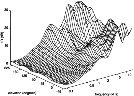
It is generally accepted that the cues used for localization are embodied in the free-field to eardrum, or head-related, transfer function (HRTF) [18]. An HRTF is a measure of the acoustic transfer function between a point in space and the eardrum of the listener. The HRTF includes the high-frequency shadowing due to the presence of the head and torso, as well as directional-dependent spectral variations imparted by the diffraction of sound waves around the pinna. The head and pinna alter the interaural cues in a frequency-dependent manner with changes in sound source position. An example of this is shown in Figure 2-1, which shows the variation of the IID with frequency and elevation along the 60° cone of confusion for a KEMAR dummy-head microphone [11].

It has been shown that HRTF data can be used effectively to synthesize localization cues in signals intended for presentation over headphones. With care, it is even possible

30 20

-a

elevation (degrees) -45 0.1 frequency (kHz)

Figure 2-1: Variations of the IID with frequency and elevation along the 600 cone of confusion (IID data derived from measurements of a KEMAR dummy-head microphone

[11]).

to achieve externalization 1 of synthesized sound sources with headphone presentation. Wightman and Kistler have shown that the information contained in the HRTFs is sufficient to explain localization performance in both azimuth and elevation [34, 35].

HRTFs vary considerably from person to person, but the types of distortions im-parted by the head and pinna follow some general patterns, so meaningful comparisons may be made. Quantitative data on "average" HRTFs and differences between listeners are presented by Shaw in [27].

At a given position, the IID and ITD can be extracted as functions of frequency from the complex ratio of the left and right ear HRTFs (i.e., the interaural spectrum).

This topic will be discussed in detail in Section 3.3.3.

2.1.4

Monaural and dynamic cues

In addition to the interaural cues described above, there are several other useful lo-calization cues, including monaural spectral cues, distance cues, and dynamic cues imparted by head movements. These cues are reviewed briefly in [18].

Spectral cues are in general related to the "shape" of the HRTF functions, possibly including the location of "ridges" and "notches" in the monaural spectrum. These cues

may be extracted by making assumptions about the source spectrum. If the source

spectrum is known, it can be "divided out" of the received spectrum. Alternatively, if

the source spectrum is not known, but can be assumed to be locally flat or of locally constant slope, the shape of the HRTF can be estimated. A computational model based on spectral cues is presented by Zakarauskas and Cynader in [38].

Localization cues for distance are not particularly well understood. The variation of signal level with distance is one potential cue, but it is useful only in regard to changes or with known source signals. The direct-to-reverberant energy ratio has also been cited as a potential localization cue, a result that stems from the fact that the reverberation level is constant over position in an enclosed space, while the direct sound energy level decreases with increasing source-to-listener distance. The ratio of high-to-low frequency energy is another prospective cue, since air attenuates high frequencies more rapidly than low frequencies over distance. To our knowledge, no models have been constructed that make use of these localization cues.

Because a slight shift in the position of the head (by rotation or "tilt") can alter the interaural spectrum in a predictable manner, head movement may provide additional cues to resolve positional ambiguities on a cone of confusion. Such cues have been dismissed by some researchers as insignificant for explaining localization performance in general, but they certainly can play a role in resolving some otherwise ambiguous

situations [18].

2.1.5

The precedence effect

In a reverberant environment, "direct" sound from a sound source arrives at a given position slightly before energy reflected from various surfaces in the acoustic space. For evolutionary reasons, it may have been important for localization to be based on the direct sound, which generally reveals the true location of the sound source [40].

Regardless of the reason of origin of the precedence effect, it is true that localization cues are weighted more heavily by the auditory system at the onsets of sounds. This temporal weighting has been observed in many contexts, and the phenomenon has been known by many names, including the "precedence effect", the "Haas effect," the "law of the first wavefront," the "first-arrival effect," and the "auditory suppression effect"

[40].

The precedence effect, as it has just been described, is a relatively short term effect, with changes in weighting operating on a time scale of milliseconds. In contrast to this, it has been shown that localization perception changes on the time scale of hundreds of milliseconds, and localization is fairly robust in the presence of reverberation, which operates on a time scale of thousands of milliseconds [40].

The mechanism that causes the precedence effect to occur is not well understood, but it has been demonstrated that it is not the result of forward masking, and that it is not due to the suppression of binaural cues alone. It has also been shown that transients (i.e., sharp changes in energy level) must be present in the sound signal for the precedence effect to occur. It is not clear how the precedence effect operates across different frequency bands [40].

Quantitative measures of the precedence effect are presented by Zurek in [39], and a model has been proposed which might explain the experimental evidence [40]. The basic form of the model is shown in Figure 2-2.

L

R

Figure 2-2: A possible model for the precedence effect, as presented by Zurek [40].

2.2 Previous work on localization models

A number of spatial hearing models have been developed. Notably, most of them fall into the "one-dimensional localization" category. These models typically estimate only a single parameter, the subjective "lateralization" of a stimulus. In this context, lateralization means "left to right position" inside the head. Recently, a few models have been constructed that are better described as "two-dimensional localization" models. These models seek to estimate both the azimuth (horizontal position) and elevation (vertical position) of sound sources. In this section, we briefly describe some of these existing models.

2.2.1

Lateralization models ("1D" localization)

Many of the early lateralization models are reviewed in [6]. Of the early models, perhaps the most influential was the neural model proposed by Jeffress ([13]), which sketches out a physiologically plausible method of extracting interaural time cues from eardrum signals. Jeffress's model was the precursor of many cross-correlation-based models, including an early one presented by Sayers and Cherry in 1957 [26].

One of the many cross-correlation-based models is the one considered by Blauert and Cobben, which employs a running, or short-time cross-correlation that operates on the outputs of band-pass channels intended to model the frequency-analysis function of the cochlea [2]. Their simple model of lateralization based on interaural time differences was extended by Lindemann to deal with interaural intensity differences and non-stationary signals, including a model of the precedence effect [16]. Gaik further extended the model by incorporating a notion of "natural" combinations of IIDs and ITDs [9]. Most recently, Bodden demonstrated that the model could be used for source separation in

a multiple-speaker speech context for sources located in the horizontal plane [3]. Another important lateralization model based on cross-correlation is the one pro-posed by Stern, Zeiberg, and Trahiotis [29, 31, 28, 32]. Their model addresses the issue of combining binaural information across frequency. As in the Blauert/Cobben model, the cross-correlation operator is applied to the outputs of band-pass filters. Stern et al. propose that the ambiguity inherent in the periodicity of narrow-band cross-correlation functions might be resolved by a "straightness" weighting of peaks across frequency.

Lateralization models typically have several limitations. Most lateralization experi-ments are performed with "unnatural" sounds, using stimuli presented on headphones,

inter-aural spectrum. These stimuli never occur in natural listening contexts, so the applica-tion of the experiments (and thus the models) to true "localizaapplica-tion" is quesapplica-tionable.2

Also, since most lateralization models deal only with statistically stationary (loosely, "steady-state") input signals, few attempt to model the precedence effect.

There are a few models that fall into the "ID" localization category without explic-itly being lateralization models. Among these is the model proposed by Macpherson, which uses a simplified model of the cochlea as a front-end for estimating azimuth and "image width" of sources in the "front half" of the horizontal plane [17]. Estimates are made from measures of the IID and ITD in various frequency bands. The model is designed to work with impulsive and continuous signals, but uses different algorithms for the two types of signals, and includes no mechanism to determine which type of signal it is operating upon. Macpherson includes a simple model of the precedence effect which operates on impulsive signals only.

2.2.2

Azimuth and elevation ("2D" localization)

Few efforts have been made to model localization in more than one dimension. Three such models, however, are the spectral-cue localization model proposed by Zakarauskas and Cynader [38], and the models based on interaural differences proposed by Wight-man, Kistler, and Perkins [36] and by Lim and Duda [15].

The model proposed by Zakarauskas and Cynader is based on the extraction of monaural cues from the spectrum received at the eardrum. They describe two algo-rithms: one which depends on the assumption that the source spectrum is locally flat, and one which depends on the assumption that the source spectrum has locally constant

slope. Both algorithms proceed to estimate the HRTF spectrum that has modified the

source spectrum. The model was able to localize sound sources in the median plane with 1 resolution, which is much better than human performance.

In [36], the authors summarize a model wherein IID spectrum templates were con-structed from HRTF data. Gaussian noise was added to these templates and the results fed to a pattern recognition algorithm in an attempt to determine if sufficient infor-mation was available to distinguish position based on the IID spectrum alone. The

authors report that discrimination was possible, and that as the available bandwidth

of the signal was reduced, localization ability was reduced in much the same manner as in humans.

The model proposed by Lim and Duda uses the outputs of a simple cochlear model to form measurements of the IID and ITD in each frequency band. The ITD mea-surements are used to estimate the azimuth of the sound source, and then the IID measurements are used to predict elevation. For impulsive sound sources in an ane-choic environment, the model is capable of 1° _{horizontal resolution and 16}° _vertical

resolution, which is comparable to the resolution exhibited by humans. The model has not yet been generalized to non-impulsive sound sources.

None of the models described in this section have attempted to model the precedence

effect.

2It has been suggested that laboratory generated distortions of IIDs and ITDs which do not arise in the "real world" may result in sound events that appear to occur inside the head [8, 9].

Chapter 3

Form of the Model

3.1 Design Overview

3.1.1

Localization cues used in the current model

As described in Chapter 2, there are several types of localization cues available. At present, monaural spectral cues are ignored, because there already exists a localization model based on them [38]. It is suggested that a spectral-cue localization model will provide an essential complement to the current model. Cues based on head movements are dismissed because of their relative non-importance ([18]) and because their use in a model precludes the use of prerecorded test signals. Distance cues, such as the direct-to-reverberant level ratio, are also ignored. Primarily, distance cues are ignored because HRTF data are assumed not to vary much with distance (regardless, HRTF data is not currently available as a function of azimuth, elevation, and distance). It is proposed that IIDs and ITDs provide sufficient cues for localization of sound sources away from the median plane. Thus, this thesis concentrates on interaural differences as the primary cues for localization.

For purposes of this thesis, the IID is defined as the difference (in dB) of the signal intensities measured at the two eardrums in response to a sound at a particular point in space. Similarly, the ITD is defined as the difference in arrival time between the signals at the two eardrums. In this thesis, IID and ITD are not single values for a given spatial location. Rather, they vary as a function of location and frequency. This distinction is important because the effects of head-shadowing and pinna diffraction are frequency dependent. Henceforth, the frequency dependent IID and ITD will be

denoted the interaural spectrum.

In this thesis, we further divide the ITD into two components, the interaural phase, or fine-structure, delay (IPD) and the interaural envelope, or gating, delay (IED). It has been shown that humans are sensitive to both types of delay [41]. The distinction is necessary because the two types of delay may vary independently in eardrum signals.

3.1.2

Block summaries

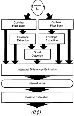
The model described in this thesis can be broken into several layers, as shown in Figure 3-1. The layers are grouped into two sections: (1) the model's "front end,"

which transforms the acoustic signals at the two eardrums into measures of interaural differences, and (2) a statistical estimator which determines the (,k) position most likely to have given rise to the measured interaural differences.

(0,0)

Figure 3-1: Block diagram of the proposed position estimator.

The structure of the model is conceptually simple. At the input, the eardrum sig-nals are passed through identical filter banks, which model the time-frequency analysis performed by the cochlea. Energy envelopes are estimated for each channel by squaring and smoothing the filter outputs. The envelope signals pass through onset detectors, which note the time and relative intensity of energy peaks in each signal. This infor-mation is used by the interaural difference estimator to model the precedence effect. The interaural difference estimators use the outputs of the filter bank, the envelope

estimators, and the onset detectors to extract the IID, IPD, and IED at onsets in each

frequency band. A "spatial likelihood" map is then generated from the interaural dif-ferences (which may be corrupted by internal "perceptual noise"), based on probability distributions for interaural differences derived from HRTF data and human psychoa-coustic data. The global maximum of the likelihood map, which corresponds to the maximum likelihood position estimate, is interpreted as the "perceived sound source

3.2 The Front End

3.2.1

Eardrum signals

The model described in this thesis operates upon acoustic signals measured at the eardrums of a listener. As it is quite difficult to make recordings of such signals, a common approach is to use an acoustic mannequin with microphones placed at the eardrums. To a good approximation, the acoustic system from a point in space to an eardrum microphone is linear, making measurement of the appropriate impulse responses and synthesis by convolution a reasonable approach to the generation of

eardrum test signals.

KEMAR HRTF measurements

Until recently, there were no publicly available impulse-response measurements of free-field to eardrum systems. To satisfy the data requirements of the current research, measurements were made of a Knowles Electronics Manikin for Acoustic Research (KEMAR). The KEMAR, fitted with a torso and two different model pinnae with eardrum microphones, was placed on a turntable in MIT's anechoic chamber. A small two-way speaker (Radio Shack model Optimus-7) was mounted, by way of a boom stand, at a 1.4 m radius from the center of the dummy-head. The speaker was posi-tioned by hand at each of 14 elevations (in 10° _{increments from -40} ° _{to 90}° _{in the}

"latitude/longitude" coordinate system). At each elevation, KEMAR was rotated un-der computer control to each azimuth measurement position (measurement positions were separated by approximately 5 great-circle arcs). Measurements were made using bursts of pseudo-random noise ("maximum-length sequences") which have the property that their autocorrelation is non-zero only at zero lag (and at multiples of the sequence length for periodically repeating signals). This property is important, as it allows the

impulse response of the system to be obtained by cross-correlation of the measured

response with the original noise signal [25, 33]. The measurement process is presented in greater detail in [10] and [11]. In total, 710 positions were measured.

Test signal synthesis

In the absence of reverberation and nearby acoustically reflective objects, the acoustic signals at the eardrums consist entirely of the direct sound from the sound source. Eardrum signals for such free-field sources may therefore be synthesized by convolution with head-related impulse-responses (HRIRs) as mentioned above.

For the experiments described in this thesis, the KEMAR HRIR measurements were used to synthesize test signals. Only the measurements of the left pinna were used, and right ear impulse responses were found by symmetry. Since the test signals required for the experiments in this thesis are for free-field signals, no more complicated synthesis techniques, such as ray-tracing or reverberation, are required.

Several types of input signals were used to test the localization model. Bursts of Gaussian white noise of various lengths, and short impulsive signals, were used to test the localization ability of the model. Also, the signals used by Zurek to quantify the

precedence effect were recreated. The results of these experiments are described in Chapter 5.

3.2.2

Cochlea filter bank

There are several issues involved in the implementation of a filter bank designed to

model the frequency analysis performed by the cochlea. These issues include the fre-quency range and resolution of the filters and their "shape."

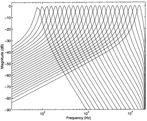
As many of the important localization cues occur in the frequency range above 4-5 kHz, the range covered by the filter bank is very important. The filter bank currently employed has center frequencies ranging from 80 Hz to 18 kHz, which covers most of the audio frequency range. The filters are spaced every third-octave, yielding 24 filter

channels in total. The third-octave spacing models the approximately logarithmic

resolution of the cochlea above 500 Hz.

All filters are fourth order IIR, with repeated conjugate-symmetric poles at the

center frequency (CF) and zeros at D.C. and at the Nyquist frequency. The pole moduli are set such that the Q of each filter (equal to the ratio of the center frequency to the -3 dB bandwidth) is 8.0, and each filter is scaled such that it has unity gain at

its CF. The constant Q nature of the filter bank is a loose fit to the critical bandwidths

reported for the human ear [19].

The "shape" of the filters is a result of the design technique, and is not intended to be a close match to cochlear tuning curves.

3.2.3

Envelope processing

There are several reasonable approaches to extracting the envelope of a band-pass signal. Three possible techniques are the Hilbert transform method, rectification-and-smoothing, and squaring-and-smoothing.

The Hilbert transform is a phase-shifting process, where all sinusoids are shifted by 900 of phase (e.g., sine to cosine). By squaring the signal and its Hilbert transform, summing the two signals, and taking the square root, the envelope signal may be

extracted.

Alternatively, the physiology of the cochlea suggests a half-wave rectification and smoothing algorithm [22]. This approach has been used by many authors (e.g., [2]), but the non-linearity of the half-wave rectifier implied by the cochlear physiology is difficult to analyze in terms of frequency domain effects and has thus not been used in

the current model.

A third alternative is the "square-and-smooth" method that is adopted in the

cur-rent model.

Assuming that we are interested in a channel that is band-pass in character with some center frequency wk (e.g., the vibration of a point on the basilar membrane), then the signal in that channel may be modeled as an amplitude modulated sinusoidal carrier:

Xk(t) = A(t) cos(wk +

q).

a)

E

2r

102 10 3 104

Frequency (Hz)

Figure 3-2: Frequency response of the filter bank used to model the frequency-analysis performed by the cochlea. Center frequencies are spaced in third-octave steps, with constant center-frequency-to-bandwidth ratio (Q = 8.0).

be low-pass in nature.

The squared signal is given by:

kx(t) = A2(t) COS2(wk + sb). (3.1)

The Fourier transform of this signal is equal to the convolution of the Fourier

transforms of the A

(t) term and the cos

(wk + ) term. Since the Fourier transform

of the cos2(Wk + ) term is the sum of three Dirac 6-functions and A2(t) is low-pass

in nature, as long as the bandwidth of the A2(t) term is less than a:k, the resulting

spectrum can be low-pass filtered at cutoff Wk, yielding the spectrum of A2(t). Further,

if A(t) is nonnegative, it may be recovered exactly by taking the square root of the resulting signal. Physically, it is impossible to realize a "brick-wall" low pass filter, but with care, the recovered A(t) is a very reasonable approximation of A(t). This concept is demonstrated in Figures 3-3 and 3-4.

In a discrete-time system, such as the implementation used in this research, aliasing is a potential problem in this processing. However, if we define BW to be the lowest frequency above which A(t) contains no energy, then as long as BW + Wk < r where 27r is the sampling frequency, there will be no aliasing. To a good approximation, this is the case for all of the filters used in this research.

There is physiological evidence that the human ear is only capable of following changes in the envelope of a signal up to an upper frequency limit. In this model,

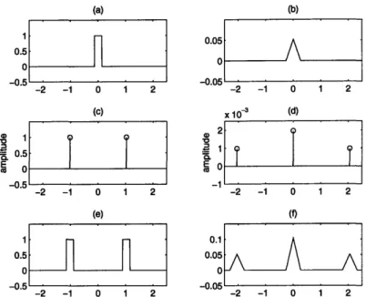
(a) (b) 0.5 0 a E co 0o -0. -2 -1 0 1 2 (c) 1-.5 .5 -2 -1 0 1 2 (e) 0.5 0 -2 -1 0 1 2

Figure 3-3: Example of Fourier spectra of x(t)

tion spectrum. All horizontal axes are in units

0.05 0 a *CL E co -2 -1 0 1 2 I'l x 10 - %u 2 . -2 -1 0 1 2 (f) 0.1 0.05 0 -2 -1 0 1 2

and x2(t) for a simple amplitude modula-of frequency divided by Wk. (a) Spectrum of A(t), (b) Spectrum of A2(t), (c) Spectrum of cos(wkt), (d) Spectrum of cos2(wkt),

(e) Spectrum of x(t) = A(t) cos(wkt), (f) Spectrum of x2(t) = A2(t) cos2(wkt). It is

possible to arrive at the spectrum in (b) by appropriate filtering of the spectrum in (f).

the limit is set to 800 Hz, which is the value chosen by Blauert and Cobben [2]. In

the implementation, this limit is imposed by not allowing the cutoff frequencies of the

smoothing filters to exceed 800 Hz.

3.2.4

Onset detection

Why onsets?

In a realistic localization scenario, the energy received at the eardrums comes from re-verberation and "distractor" sound sources as well as directly from the "target" source. Sharp peaks in energy that may be attributed to the target source generally provide small time windows with locally high signal-to-noise ratios for estimating attributes of the source signal (e.g., interaural differences).

As mentioned previously, there is evidence that onsets are particularly important portions of the signal for purposes of localization. This is demonstrated by their im-portance in relation to the precedence effect [40].

Extraction method

The model searches for energy peaks in the various filter bank channels by looking for maxima in the envelope signals. These "onsets" are found by a simple peak-picking

algorithm coupled with a suppression mechanism. In the current implementation, the

envelope signals at the two ears are summed before onsets are detected; thus, onsets are

-n li . . . -- I!.- i i i i . .* . . . I ,_.-~ Lin n

il

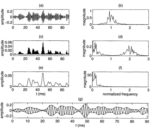
(a) 0 20 40 60 80 (c) 0 20 40 60 80 (e) 20 40 t (ms) 1) -E 1 a c 0.5 a) ' 0.2 C 0 1 2 3 (d) 3 0 1 2 3 (f) n U) 5 c E 60 80 0 1 2 normalized frequency (g) I I Iii i i I I I I I 10 20 30 40 50 60 70 80 90 t(ms)

Figure 3-4: Example of the envelope extraction process for a band-pass signal. The normalized frequency axis is in units of frequency divided by k. (a) Time waveform of the bandpass k(t), (b) Spectrum of k(t), (c) Time waveform of x(t), (d) Spectrum

of x(t), (e) Time waveform of A2_{(t), (f) Spectrum of A}2_{(t). (g) Time waveform of}

the bandpass k(t) with A(t) and -A(t) superimposed. Since the frequency axis is

normalized and the filter bank used in this research is constant Q, the above plots are typical of all frequency channels, with an appropriate scaling of the time axis.

C 0.2 0 , -0.2 - 0.06 ' 0.04 a0.02 O co 0 a) 0 0.05 E U 0 0 -o 0.2-o 0 E _0.2I 0 . . . _ . . . II . . (b) r L

.

Las

M*"

not independently found at the two ears. The model proposed by Zurek (see Figure 2-2) suggests that a sharp onset should suppress localization information (including other onsets) occurring over approximately the next 10 ms [40]. In the current model, a small backward-masking effect has been implemented to ensure that a false-alarm is not triggered by a small onset when it is immediately followed by a much larger one.

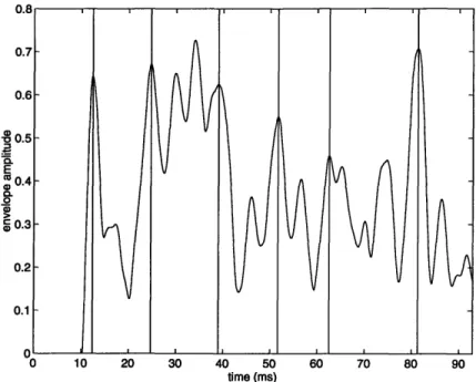
Figure 3-5 shows an example of onsets detected in an envelope signal which has been extracted from a channel with a center frequency of 800 Hz.

0 10 20 30 40 50 60 70 80 90 time (ms)

Figure 3-5: Example of onsets extracted from an a center frequency of 800 Hz. Some of the local maximum) have been suppressed in this example.

envelope signal in a channel with maxima (and, in fact, the global

3.2.5

Interaural differences estimation

Interaural intensity differences

In the current model, the IID is simply formed by the log ratio of the envelope signals:

IIDk(t) =

0 loglo(ER,k(t)/EL,k(t)),

With the current IID formulation, an interesting artifact occurs that is due to the

coupling of IID and ITD in natural listening situations. IID and ITD tend to co-vary for single sound sources in free-field. This fact follows directly from the form of natural HRIRs, which dictate that an energy burst will excite the ipsilateral (near-side) ear

more intensely and sooner than the contralateral (far-side) ear. Similarly, an energy

offset will cause the excitation at the ipsilateral ear to drop off before the excitation

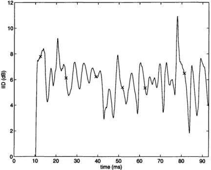
drops off at the contralateral ear (it should be noted that this time lag is in general smaller than 1 ms). Because of this effect, a sharp energy peak in the input signal will cause fluctuations in the output of the IID estimator. This effect can be seen in Figure 3-6, which shows the IID trace for the same signal as was used to generate Figure 3-5. This effect will be described further in Section 4.1, which treats the issue of measurement noise.

en

0 10 20 30 40 50 60 70 80 90 time (ms)

Figure 3-6: Example showing variation of the IID function over time for a time-varying input spectrum. Each (x) marks the position of an onset detected in the signal (see Figure 3-5).

Interaural phase delays

The IPD is estimated by a running cross-correlator similar to those proposed by Blauert

[2] and Lindemann [16]:

IPD(t) = argmax

Lk(t'

)Rk(t'

+)w(t-

t)dt'.

Here, Lk(t) and Rk(t) are the signals in the kth channel of the left and right ear filter banks respectively, w(t) is a window function, and r is limited to the range -1 < r < 1 ms, which includes the range of IPDs encountered in natural listening conditions. The window used by Blauert is a decaying exponential with a time constant

of a few milliseconds [2]. In the current model, we use a window of the form:

w(t) = Ate

7,

(3.4)

with an effective "width" of 4-5 ms.

In the current implementation, the running cross-correlation is sampled in r. The sampling is performed in approximately 45 ps increments (which corresponds to two sample periods at a 44.1 kHz sampling rate) over the -1 < r < 1 ms range. The peak in

the cross-correlation function is then interpolated by a quadratic fit to the three points

surrounding the global maximum. This process breaks down due to under-sampling (of r) for filters with center frequencies that are larger than approximately 1.5 kHz. Since humans are incapable of fine structure analysis above 1.5 kHz ([19]), this breakdown is acceptable, and the IPD is not evaluated in channels with center frequencies larger than 1.5 kHz.

The cross-correlation of a narrow-band signal is nearly periodic in r, with period equal to the inverse of the carrier frequency of the signal. This near-periodicity, which is present in the cross-correlations of band-pass signals in the cochlear filter-bank, makes extraction of the interaural delay a difficult task, with "period" errors common. The effect of introducing a time-limited window into the cross-correlation is to reduce the size of cross-correlation peaks at lags distant from zero. Since interaural delays tend to fall in range -1 < r < 1 ms, we may largely ignore cross-correlation peaks at lags outside of this range.

Interaural envelope delays

The IED estimation is identical to the IPD estimation, except that the envelope signals, EL,k(t) and ER,k(t), are substituted for the filter bank signals in Equation 3.3. In general, the two window functions w(t) used for the IPD and IED estimators may be different, but the same window is used presently for the sake of simplicity. Since the envelope signals are low pass in nature, under-sampling of the cross-correlation function is not an issue.

3.3 Position Estimation

3.3.1

Precedence effect model

The precedence effect model is based upon the one proposed by Zurek (see Figure 2-2 and [40]). We assume that the inhibition (or suppression) described in the model

applies to the localization cues, rather than an actual position estimate. Further, we

make the assumption that the inhibition operates independently in the various filter-bank channels. It is unknown whether these assumptions are valid.

The onset detector described in Section 3.2.4 provides a time-stamped list of "on-sets" detected in each filter channel. It is assumed that each detected onset causes a sampling of the interaural difference signals derived from the appropriate filter channel. The sampling function (or window) is positioned in time such that the main lobe is

inner product of the window function with the appropriate running interaural differ-ence signal (as described in Section 3.2.5). The window function is scaled such that it integrates to unity, which ensures that the measured value is correct for a constant interaural difference signal.

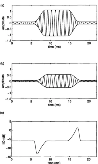
The form of the sampling function is chosen to approximately match the inhibition curve sketched by Zurek (see Figure 3-7a). The window takes the form in Equation 3.4, with set to make the effective window "width" approximately 2-3 ms. The sharp drop in sensitivity is assumed to be due to the shape of the sampling function (as shown in Figure 3-7b), while the limitation imposed by the onset detector (that onsets occur no more frequently than one every 10 ms) is assumed to account for the return of sensitivity approximately 10 ms following an onset.

.5

'a)_'

Figure 3-7: (a) Inhibition curve for localization information suggested by Zurek. (b) Sampling window used in the model (of the form w(t) = Atexp(-t/r)).

Some results of experiments testing the adequacy of this implementation are pre-sented in Chapter 5.

3.3.2

Development of the position estimator

If we make the restriction that the model has no a priori knowledge of the input spectrum, we might assume, for purposes of constructing a model, that the "average" spectrum is locally "white" (i.e., that the probability distribution of input signal energy is constant over frequency). We can then argue that the interaural differences for a source at a given position will vary in a noise-like manner about some mean as changes in the input spectrum interact with the fine structure of the HRTFs within any given band-pass channel. We further make the doubtful, but nonetheless common, assumption that the noise is additive, Gaussian, and zero-mean in nature.

With these assumptions, we may write the probabilistic formulation:

P = P, + ,

(3.5)

where

v

.A(O,

(3.6)

Here, P is a vector consisting of the various interaural measurements under consider-ation, Pe,, is the expected value of P, given that the sound source is at the location (0, q), and v is the additive noise vector, which is Gaussian with covariance matrix K. With n interaural difference measurements, P, P0,0, and v are (n x 1) and K is (n x n).

The probability density function for P, given (0, 'k), is then Gaussian with mean P,o

and covariance K:

P N

A(P,o, K),

(3.7)

p(P[I,b)

= (2r)n/2 K1

_{exp - 2(P - P,)TK/-(P-}

_)}

_(3.8)

If we also assume that the noise in each interaural difference measurement is

inde-pendent of the noise in the other measurements, then the matrix K is diagonal:

2

2 a2

K

(3.9)

Here, E2 is the variance of the noise in the kth measurement (noise in the model is examined in depth in Chapter 4).

With this formulation, we may write a simplified equation which represents the

likelihood that the measurements arose from a source at location (, q):

Cs,+

= p(P1 +)=

exp {-

(Pk - P,,k)}

(3.10)

(2)n12

J

(ok{

k=1

rk

k=1

It is worth noting at this point that ak is assumed to be constant over all (, q) positions, which makes the term multiplying the exponential a constant over all po-sitions. It is therefore quite straightforward to compare the "likelihoods" at different positions, based on the observed measurements.

By calculating Co,+ at a number of different positions, it is possible to generate a

spatial likelihood map, which shows the relative likelihood that the sound source is at

each position. Examples of spatial likelihood maps are given in Chapter 5.

3.3.3

Template extraction from HRTF data

In order to calculate the likelihood function for a particular position, the mean values for the interaural differences for a source at that position are required. Reapplying

the input signal assumptions that we used to derive the probabilistic model, we may extract the expected mean values of the interaural differences from HRTF data by making some assumptions about the types of input signals that the system is likely to encounter.

The assumptions that we choose to make are that the average spectrum is "white" (i.e., the probability distribution for input signal energy is constant over all frequencies of interest). When the time-structure of the input signal is required in the template calculations, we assume that the signal is impulse-like (i.e., it is time-limited, with short duration), and we in fact use the Dirac 6-function to represent the input.

Interaural intensity differences

We may consider the envelope extraction process to derive the IID template func-tion. For a single free-field sound source at position (, q), the signals received at the eardrums are given by:

L(t)

=

x(t) * h(t)

(3.11)

R(t) = x(t) * hR(t),

(3.12)

where L(t) and R(t) are the signals received at the left and right eardrums respec-tively, x(t) is the source input signal, and hL(t) and h (t) are the left and right ear HRIRs respectively. In these equations and those that follow, * denotes the convolution

operator.

The squared envelope signals extracted from these input signals are then given by:

EL,k(t)

=

(L(t) * hk(t))

* hE(t)

(3.13)

ER,k(t)

=

(R(t)

hk(t))

h(t),

(3.14)

where EL,k(t) and ER,k(t) are respectively the left and right side envelope signals in the kth band-pass channel, hk(t) is the impulse response of the kth band-pass filter, and

hE(t) is the impulse response of the smoothing filter used in the envelope extraction

process in the kth channel.

We may then form the following expression for the IID:

IIDk,e,4(t) =

w(t' - t)10 log

(3.15)

where w(t) is the window function described in Section 3.3.1. We must be careful to

en-sure that EL,k(t) and

are always non-zero, but due to the IIR nature of the filter

bank, once the filters have been initially excited, this condition is generally satisfied. Regardless, a simple threshold mechanism would suffice to correct this problem.

Assuming an impulse-like input signal (a Dirac 6-function in the limit), we may

form the IID template function:

IIDk,e,4(t) =

w(t' - t)101log

(

(t

hk(t))2

)

dt'

(3.16)

Interaural phase delays

For a known input signal, the IPD is given by Equation 3.3. If we again assume that the input is an impulse, we may construct the IPD template as follows:

Lk,o,(t)

Rk,O,O(t)

= hk(t) *

ho(t)

(3.18)

IP'r9,)t

=

2)w(t' - t)dt' (3.19)

IPDk-,o,¢(t) =

argmax

Interaural envelope delays

In the same fashion as we constructed the IPD template, we may construct a template

for the IED:

Ek(t

= (hk(t) *

ho(t))

*

h

(t)

(3.20)

ER2,o(t)

(hk(t)

h R(t))

h(t)

(3.21)

r00

IEDk,o,O(t)

=

argmax

EkL (t'-

)

( +

w(t' -

t)dt'

(3.22)

-OO2

3.3.4

Spherical interpolation

We would like to calculate spatial likelihood maps that are much more densely sampled

in azimuth and elevation than the KEMAR HRTF data. Without a dense sampling,

it is difficult to measure localization errors quantitatively, because many errors will be due to the measurement position quantization. There are two possible approaches to solving this problem: (1) interpolation of the spatial map derived from interaural difference templates at KEMAR measurement positions only, and (2) interpolation of

the interaural difference templates themselves. If the interaural difference templates are

relatively smooth functions of position (which seems to be the case), then the second method is clearly preferable.

Interpolation of functions in spherical coordinate systems is a difficult problem, however. The KEMAR HRTF data set is not sampled regularly (i.e., the sample points are not located at the vertices of a polyhedron); therefore, the interaural differ-ence templates are also irregularly sampled. There are many possible approaches to the "spherical interpolation" problem, including minimum mean-square error (MMSE) interpolation with some basis function set defined under spherical coordinates.

The MMSE method is a well-known functional approximation technique using basis functions. First, we define an inner product in our coordinate system:

<

x(,

), (O, ) >=

JJ

x(O,)y(O,

)dA,

(3.23)

where < x(0, q), y(0, q) > is the inner product of two functions, x and y, defined in our coordinate system, and the integral is evaluated over the range of possible (, 4) values. It should be noted that we have stated this problem in terms of spherical coordinates, but it is equally applicable to problems in other coordinate systems. The only change in Equation 3.23 is the form of the dA term (and possibly the number of integrals). Henceforth, we will use the angle bracket notation introduced above to represent the

inner product.

Next, we define a set of basis functions, Lk(0, 4), k = 1 ... N, which will be used

to approximate the function d(O, 4):

N

d(o,

=

W)

kk(0, ).

(3.24)

k=l

With this formulation, the weights

which minimize the mean-squared error:

E=

JJ/

R

are given by the solution of:

<

>

< .,

< 1,

>

w

-

l,d>

.' .. .. : · = :.

.

(3.26)

< N, Il l > ... < N , N > WN < N,

d

>

In this thesis, we are interested in finding smooth approximations to the interaural difference functions. Since the interaural differences are only measured at discrete (0, 4) positions, we approximate the continuous integral in Equation 3.23 by the following discrete summation:

<

, y

>_

E XkYkAk.

(3.27)

k

Here, k indexes the various measurement positions, xk and Yk are the values of x(O, 4) and y(O, 4) at position k, and Ak is the "area" represented by measurement position

k. For the training positions used to estimate the interaural difference surfaces (the

positions are separated by roughly 10° _{great circle arcs), we have Ak - K, for all k.}

Thus, the Ak term may be ignored in Equation 3.27.

For our basis functions, we define a set of "spherical Gaussian" functions of the form:

Xk(P)

= exp [-

(p

Pk)],

(3.28)

where (p - Pk) is defined as the great circle arc (in degrees) between positions p and Pk. We define p and Pk to be positions on a sphere, each indexed by azimuth and elevation in a convenient spherical coordinate system. In Equation 3.28, K is a smoothing factor (chosen in this thesis to be 120 degrees-squared). With this formu-lation, the basis function is unity at its kernel position, Pk, and falls off by a factor of 1/e for each v'1h2 ~ 11° distance increment. In Appendix A, Figure A-2 shows