A compressed sensing approach to the simultaneous recording of multiple room impulse responses

(1)

HAL Id: hal-00612911

https://hal.archives-ouvertes.fr/hal-00612911v2

Submitted on 5 Aug 2011

HAL is a multi-disciplinary open access

archive for the deposit and dissemination of

sci-entific research documents, whether they are

pub-lished or not. The documents may come from

teaching and research institutions in France or

abroad, or from public or private research centers.

L’archive ouverte pluridisciplinaire HAL, est

destinée au dépôt et à la diffusion de documents

scientifiques de niveau recherche, publiés ou non,

émanant des établissements d’enseignement et de

recherche français ou étrangers, des laboratoires

publics ou privés.

recording of multiple room impulse responses

Alexis Benichoux, Emmanuel Vincent, Rémi Gribonval

To cite this version:

Alexis Benichoux, Emmanuel Vincent, Rémi Gribonval. A compressed sensing approach to the

si-multaneous recording of multiple room impulse responses. IEEE Workshop on Applications of Signal

Processing to Audio and Acoustics, Oct 2011, New Paltz, NY, United States. pp.1. �hal-00612911v2�

(2)

A COMPRESSED SENSING APPROACH TO THE SIMULTANEOUS

RECORDING OF MULTIPLE ROOM IMPULSE RESPONSES

Alexis Benichoux

Universit´e Rennes 1, IRISA - UMR6074

Campus de Beaulieu 35042 Rennes, FR

alexis.benichoux@irisa.fr

Emmanuel Vincent, R´emi Gribonval

INRIA, Centre de Rennes - Bretagne Atlantique

Campus de Beaulieu 35042 Rennes, FR

{emmanuel.vincent, remi.gribonval}@inria.fr

ABSTRACT

We consider the estimation of multiple room impulse responses from the simultaneous recording of several known sources. Existing techniques are restricted to the case where the number of sources is at most equal to the number of sensors. We relax this assumption in the case where the sources are known. To this aim, we propose sta-tistical models of the filters associated with convex log-likelihoods, and we propose a convex optimization algorithm to solve the in-verse problem with the resulting penalties. We provide a compari-son between penalties via a set of experiments which shows that our method allows to speed up the recording process with a controlled quality tradeoff.

Index Terms— Room impulse response recording, convex

op-timization, compressed sensing

1. INTRODUCTION

We focus on the recording of multiple room impulse responses. Up to now this is typically achieved by activating each loudspeaker or source in turn, with a silent interval equal to the expected du-ration of the impulse response in between [1]. The total record-ing duration is thenN (D + K − 1) where N is the number of sources,D the chirp duration and K the impulse response length in samples. An improvement [2] is to use time-overlapping but time-frequency disjoint chirps, which reduces the recording dura-tion down toN K + D − 1 when the system is linear. These tech-niques remain time-consuming e.g. in the context of the calibration of high-end 3D audio systems or the collection of binaural room im-pulse responses involving hundreds of loudspeakers. We investigate here possible improvements using state-of-the-art system inversion tools. This problem is equivalent to the estimation of the mixing

filtersin the context of convolutive source separation [3].

The techniques in [4] and [3] for mixing filter estimation as-sume each source to be active alone in a certain time interval. Once this time interval has been localized, the corresponding fil-ters are estimated using a subspace method [4], or convex optimiza-tion [3]. Alternative Convolutive Independent Component Analysis techniques [5] assume the number of sources to be at most equal to the number of sensors. Our work is to our knowledge the first to get rid of these two assumptions. We propose to take advantage of the a priori temporal structure of the filters to improve the iterative inversion of the linear system. In addition to the sparse prior intro-duced in [6] for single-source blind channel identification, we pro-pose four new priors and a new multi-source inversion algorithm. Our approach is an example of compressed sensing [7][8], that is an emerging general approach to the recovery of structured signals

from a smaller number of measurements. We show theoretically that white noise sources provide the most convenient system for in-version.

The structure of the paper is as follows. The formalization of the problem is described section 2. Section 3 corresponds to the study of the a priori structure of the filters. The implementation of the algorithm is detailed Section 4. The results shown in Section 5 show the potential of the proposed method.

2. APPROACH

The problem is formalized as follows : we represent theN sources of length_{T by the matrix S ∈ R}N ×T, the filters of lengthK by the three dimensional array A ∈ RM ×N ×K _{and the}_{M observations}

by X∈ RM ×(T +K−1). Assuming that the loudspeaker are linear, the convolutive matrix product⋆ allows us to write

X= A ⋆ S = 0 @ X n≤N Amn∗ Sn 1 A m≤M . (1)

Earlier work [9] used convex optimization tools to recover S when A is known, using a sparsity prior on the sources.

Here we adapt the method in [9] to estimate A when S is known, by estimatinglimλ→0Aλwhere

Aλ= argminA  1 2kX − A ⋆ Sk 2 2+ λP(A) ﬀ . (2)

This limit is the solution of the constrained minimization problem min

A P(A) s.t. kX − A ⋆ Sk 2

2= 0. (3)

We choose for_{P the negative log-likelihood of a distribution} sug-gested by the statistical analysis of a large family of filters.

3. STATISTICAL ANALYSIS OF A FAMILY OF FILTERS

The statistical theory of room acoustics [10] treats each filter as a random i.i.d. signal whose amplitude envelopeρ(t) decays expo-nentially according to

ρ(t) = σ 10−3t/tR

, (4)

wheretRis the room reverberation time in samples, andσ a scaling

factor. This theory assumes that a filterA ∈ RK_{follows a Gaussian}

distribution. In other work [6],A(t) is instead assumed to have a constant amplitude envelope and to be sparse, as it is formed by

(3)

0 50 100 150 200 250 2 3 4 5 6 7 8 t (ms) log−likelihhod P₁ P2 P3 P4

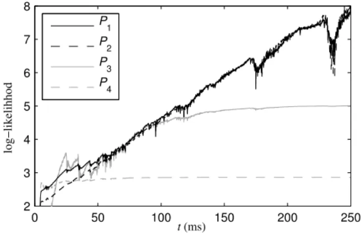
Figure 1: Comparison of the statistical models (5) to (8) over a set of generated filters for a reverberation time of250 ms.

echoes at distinct instants. In order to evaluate the respective impact of both the envelope model and the sparsity model, we consider the following distributions : Laplacian with decaying envelope

P1(t) =

1 2ρ(t)e

−|A(t)|/ρ(t)_,

(5) Gaussian with decaying envelope

P2(t) = 1 √ 2πρ(t)e −A2 (t)/2ρ2 (t)_, (6) Laplacian with constant envelope

P3(t) =

1 2σe

−|A(t)|/σ_,

(7) Gaussian with constant envelope

P4(t) = 1 √ 2πσe −A2 (t)/2σ2 . (8)

Figure 1 compares the average negative log-likelihoods of these four models over a set of 10 000 filters simulated by the image method [11] for one source and one microphone at random positions spaced by1 m, in a rectangular room of dimensions 10 × 8 × 4 m withtR = 250 ms. For each model, the scaling factor σ is set in

the maximum likelihood sense. Envelope modeling appears to be crucial : the likelihood of modelsP3andP4 is much larger than

that ofP1andP2 for larget. Sparsity has a weaker impact : the

likelihood ofP1(and to a lesser extent that ofP2) is larger than that

ofP2 fort ≤ 60 ms, but becomes similar for t > 60 ms. These

observations lead us to propose a fifth hybrid model

P5(t) =

(

P1(t) ift ≤ 60 ms

P2(t) it > 60 ms.

(9)

Assuming Gaussian white additive noise, maximum

a posteriori estimation of the filters is equivalent to (2) with Pi= − log Pi.

4. ALGORITHM

To solve (2), we use the FISTA (Fast Iterative Shrinkage-Thresholding) algorithm [12], which exploits the differentiability

of the data fidelity term

L : A 7→ kX − A ⋆ Sk22, (10)

and the convexity and semicontinuity ofPi. So-called proximity

operators are employed to overcome the non-differentiability ofPi.

Definition 1 ForP : E → R semicontinuous and convex the

prox-imity operator associated withP is the function prox_P: x ∈ E 7→ argminy∈E



P(y) +1₂kx − yk22

ﬀ

The general steps of FISTA are described in Algorithm 1. It relies on the computation of the gradient of_{L, its Lipschitz constant L,} and the proximity operator of the scaled penaltyαP.

Algorithm 1 FISTA 1: A0∈ RM N K, τ0= 1 2: fork ≤ kmaxdo ˜ Ak= proxλ LP “ Ak−1−∇L(ALk−1) ” τk₌ 1+√1+4(τk−1)2 2 Ak= ˜Ak+τk−1₋₁ τk ( ˜A k_{− ˜}_Ak−1₎ 3: end for

The computation of the gradient ofL requires the introduction of the adjoint of the linear operator A7→ A ⋆ S. Denoting by ˜Sn∈

RTthe time reversal ofSn, i.e. fort ≤ T , ˜Sn(t) = Sn(T − t + 1),

the adjoint operator is expressed usingS∗_:=“ ˜_S

1, . . . , ˜SN ” as X_{7→ X ⋆ S}∗:=“( ˜Sn∗ Xm)(t) ” m≤M,n≤N,1≤t≤K. (11)

One may then write the gradient as

∇L(A) = (X − A ⋆ S) ⋆ S∗. (12) The Lipschitz constant of∇L is the greatest eigenvalue of the oper-ator A7→ A⋆S⋆S∗_{. We obtain this value using the power iteration}

algorithm as in [9, Algorithm 5].

The log-likelihood of the distributions introduced previously correspond to theℓ1andℓ2norms, whose proximity operators are

Concerning the hybrid model (9), we use (13) or (14) depending on the value oft.

We estimate the minima Aλforλ ∈ {1, 10−1, . . . , 10−14},

initializing each FISTA step at the minimum obtained for the previ-ous value. We keep the last minimum obtained forλ = 10−14, and consider it as an estimate of the limitlimλ→0Aλ, i.e. the solution

of (3). Note that theℓ2penalizationP4corresponds to the definition

(4)

450 650 850 1050 1250 1450 0 10 20 30 40 50 60 70 Inf overdetermined underdetermined T c →

Duration T+K−1 of the recording (ms)

SNR A out (dB) P1 P2 P3 P4 P5

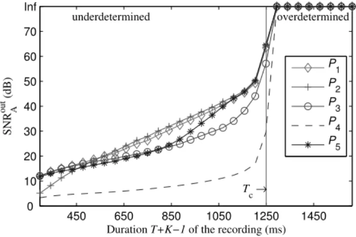
Figure 2: Performance of the estimation of A withN = 5 white noise sources, depending on the duration of the signal.

5. EXPERIMENTAL RESULTS

The Matlab code allowing to reproduce the following experiments is available at the following address [13].

5.1. Role of the condition number

First we wish to study the contribution of the penalty depending of the invertibility of the problem. The system is composed of M (T +K −1) equations for MNK variables, therefore it is under-determined if and only if the recording duration in samples satisfies T + K − 1 < Tc:= N K. (17)

Note thatTcis smaller thanN K + D − 1 which is the length of the

recording required in [2].

Performance does not depend on the number M of micro-phones, in fact each microphone brings an independent problem.

The_{M N filters are a solution of the linear system, for m ≤ M} Xm= S1⋆ Am1+ S2⋆ Am2+ . . . + SN⋆ AmN. (18)

In order to guide the choice of the source signals, we first show theoretically that the system is well conditioned if the sources are uncorrelated. To this aim we compute the condition number of the system i.e. the ratio of highest to lowest singular value. Note that this is only defined for a full rank system, hence forT ≥ Tc. In the

under-determined setting, similar estimates can easily be obtained by exploiting the sparsity of the filters A.

The relation between the correlation of the sources and the con-dition number of the system is detailed in the following lemma proved in the Appendix. Using the usual cross-correlation function forn, n′_{≤ N :} rnn′(k) = T −k X t=1 Sn(t)Sn′(t + k), 0 ≤ k ≤ K − 1. (19)

we introduce a measure of the maximum correlation between the sources r := max n6=n′or k6=0|rnn′(k)|, (20) 450 650 850 1050 1250 1450 0 10 20 30 40 50 60 70 80 30dB 40dB 50dB 60dB 70dB 80dB overdetermined underdetermined T c →

Duration T+K−1 of the recording (ms)

SNR

A

out

(dB) P1

P4

Figure 3: Estimation of A for six different additive noise levels, depending on the recording duration withN = 5 sources

Lemma 1 For smallr, the condition number of (18) obeys 1 ≤ c ≤maxnrnn(0) + r(N K − 1)

minnrnn(0) − r(NK − 1)

. (21)

Note that for white noises,r is small, and c is close to 1, leading to a well conditioned system.

5.2. Performance as a function of the recording duration

In previous work [14, fig.2], we used human voice recordings, and we observed a transitory regime forT > Tc where the penalties

still had an impact due to a large condition number. In this paper we want to choose the sources such that the system is well-conditioned, therefore we used white Gaussian noise, motivated by the above the-oretical guarantees. We observed experimentally (results not shown here) that this choice remains experimentally valid for underdeter-mined systems.

As a measurement of the error between the estimated filters Aλ

and the true filters A, we define the following ratio in decibels SNRoutA (Aλ) = 10 log10 kAk

2 2

kAλ− Ak22

. (22)

When the solution is not unique, we expect to observe better results with the proposed regularizations : we then run the algorithm for several values ofT .

The results shown in Figure 2 correspond to the case ofN = 5 sources,M = 2 sensors, with filters of length K = 2753 (250 ms sampled at11025 Hz) synthesized as in Section 2. For readabil-ity we express all the durations in ms the following. We obtain the critical valueTc = 1250 ms beyond which the system is

overde-termined. We vary the length of the sources fromT = 45 ms to T = 1500 ms.

We observe in Figure 2 a clear jump around the critical valueTc

after which the inversion made by all regularized algorithms yields the same solution, up to machine precision.

For T < Tc we observe the clear impact of all

regulariza-tions compared to the pseudo-inverseP4. The new penaltiesP1

andP2, corresponding to the Laplacian and Gaussian distributions

with decaying envelope give the best results. For a speed-up of 50% in recording duration compared to [2], we achieve a recovery SNRoutA = 25 dB.

(5)

5.3. Robustness to noise

We now add Gaussian white additive noise to the mixtures,

X= A ⋆ S + W. (23)

For each penaltyPiand each durationT + K − 1 of the

record-ings, six experiments were made for a signal-to-noise ratio of 30, 40, 50, 60, 70 and 80 dB. We observe in Figure 3 that the noise decreases the overall performance, but has a smaller impact on the ℓ1re-scaled penaltyP1than on the common pseudo-inversionP4.

Not surprisingly, the two penalties lead to the same result once the sources are long enough for the solution to be unique.

This experiment confirms the possibility to speedup the record-ings even in the presence of noise. With an input SNR of50 dB, the estimation fidelity SNRoutA is still25 dB.

6. CONCLUSION

For the considered problem, the various a priori introduced as con-vex penalties provide better estimation of the filters than simple de-convolution using Moore-Penrose pseudo-inverse. The best results are achieved with the new proposed penalties based on a decay-ing envelope model. This method can speed up the recorddecay-ing, with a reasonable quality trade-off for noisy measurements. For large numbers of sourcesN in reverberant rooms, the expected speedup can be significant. Further experiments are needed to confirm the validity of the approach in such scenarii, by taking into account the nonlinearity of the loudspeakers, as well as other performance mea-sures. Besides, we know that source separation informed by the filters provides better results [9] : this opens the way to the alternate estimation of both the sources and the filters with suitable penalties on the filters as opposed to [15].

Appendix

Denote Σn:= 0 B B B B B B B B B B B @ Sn(1) 0 · · · 0 .. . . .. . .. ... 0 Sn(T ) Sn(1) 0 . .. .. . . .. ... 0 · · · 0 Sn(T ) 1 C C C C C C C C C C C A ∈ R(T +K−1)×K.

We derive from (18) the block matrix notation

(ΣTnXm)n≤N = (ΣTnΣn′)n,n′≤N(Amn)n≤N, (24)

and the correlation of the sources (19) appears since we have

ΣTnΣn′ = 0 B @ rnn′(0) · · · rn′n(K − 1) .. . . .. ... rnn′(K − 1) · · · rnn′(0) 1 C A. (25)

Now_{c is the condition number of the N K × NK block matrix} R= (ΣT

nΣn′)n,n′≤N, and the key is to choose the sources so that

This work was supported by the EU FET-Open project FP7-ICT-225913-SMALL and the ANR project 08-EMER-006 ECHANGE.

this matrix is highly diagonally dominant. Using Gerschogorin’s disc theorem [16], we control its eigenvalues. Forλ ∈ Sp(R), there existn ≤ N such that

|λ − rnn(0)| ≤ K−1 X k=1 rnn(k) + K−1 X k=0 X n6=n′ r (26) ≤ r(NK − 1) (27)

Then ifr(N K − 1) < minnrnn(0) we can conclude that

c = |λmax| |λmin| ≤ maxnrnn(0) + r(N K − 1) minnrnn(0) − r(NK − 1) . (28) 7. REFERENCES

[1] A. Farina, “Simultaneous measurement of impulse response and distortion with a swept-sine technique,” in Proc. AES

108th Convention.

[2] P. Majdak, P. Balazs, and B. Laback, “Multiple exponential sweep method for fast measurement of head-related transfer functions,” Journal Audio Engeneering Society.

[3] P. Sudhakar, S. Arberet, and R. Gribonval, “Double sparsity: Towards blind estimation of multiple channels,” in Proc. Int.

Conf. on Latent Variable Analysis and Signal Separation. [4] A. Aissa-El-Bey, K. Abed-Meraim, and Y. Grenier, “Blind

separation of underdetermined convolutive mixtures using their time-frequency representation,” IEEE Transactions on

Audio Speech and Language Processing.

[5] S. Makino, T. Lee, and H. Sawada, Blind speech separation. [6] Y. Lin, J. Chen, Y. Kim, and D. Lee, “Blind channel

identifi-cation for speech dereverberation usingℓ1-norm sparse

learn-ing,” in Advances in Neural Information Processing Systems

20.

[7] D. Donoho, “Compressed sensing,” Information Theory, IEEE

Transactions on.

[8] E. Cand`es, “Compressive sampling,” in Proceedings of the

In-ternational Congress of Mathematicians. Citeseer.

[9] M. Kowalski, E. Vincent, and R. Gribonval, “Beyond the narrowband approximation: Wideband convex methods for under-determined reverberant audio source separation,” IEEE

Transactions on Audio, Speech, and Language Processing. [10] H. Kuttruff, Room Acoustics, 4th ed., New York.

[11] J. Allen and A. Berkeley, “Image method for efficiently simu-lating small-room acoustics,” Journal of the Acoustical

Soci-ety of America, Apr.

[12] A. Beck and M. Teboulle, “A fast iterative shrinkage-thresholding algorithm for linear inverse problems,” SIAM

Journal on Imaging Sciences. [13] http://hal.inria.fr/inria-00594252/.

[14] A. Benichoux, E. Vincent, and R. Gribonval, “Optimisa-tion convexe pour l’estima“Optimisa-tion simultan´ee de r´eponses acous-tiques,” in Actes du23e_{colloque GRETSI}_.

[15] D. Barchiesi and M. D. Plumbley, “Dictionary learning of con-volved signals,” In Proc. Conf. on Acoustics, Speech and

Sig-nal Processing.