Concepts and technology development for the autonomous assembly and reconfiguration of modular space systems

(1)

Concepts and Technology Development for the Autonomous Assembly and Reconfiguration of Modular Space Systems

by

Lennon Patrick Rodgers

B.S. Mechanical Engineering

University of Illinois at Urbana-Champaign, 2003

Submitted to the Department of Mechanical Engineering in partial fulfillment of the requirements for the degree of

Master of Science in Mechanical Engineering at the

Massachusetts Institute of Technology February 2006

Signature of Author:

Department of Mechanical Engineering December 20, 2005

Certified by:

David W. Miller Professor of Aeronutics and Astronautics Thesis/ dvisor

Accepted by:

Warren Se ring Professor of Mechanical Engin ering Thesis Reader

Accepted by:

Lallit Anand

____________________ Professor of Mechanical Engineering

MASSACHUSETTS IN TITE _{Chairman, Committee on Graduate Students}

(2)

M

nITLIbrries

Document Services Room 14-0551 77 Massachusetts Avenue Cambridge, MA 02139 Ph: 617.253.2800 Email: docs@mit.edu http://Iibraries.mit.edu/docs

DISCLAIMER OF QUALITY

Due to the condition of the original material, there are unavoidable flaws in this reproduction. We have made every effort possible to

provide you with the best copy available. If you are dissatisfied with this product and find it unusable, please contact Document Services as

soon as possible. Thank you.

The images contained in this document are of

the best quality available.

(3)

(4)

Concepts and Technology Development for the Autonomous Assembly and Reconfiguration of Modular Space Systems

by

Lennon Patrick Rodgers

Submitted to the Department of Mechanical Engineering on December 20, 2005, in partial fulfillment of the requirements for the degree of Master of Science

Abstract:

This thesis will present concepts of modular space systems, including definitions and specific examples of how modularity has been incorporated into past and present space missions. In addition, it will present two architectures that utilize modularity in more detail to serve as examples of possible applications.

The first example is a fully modular spacecraft design, which has standardized and reconfigurable components with multiple decoupled subsystems. This concept was developed into a testbed called Self-assembling Wireless Autonomous and Reconfigurable Modules (SWARM). This project sought to demonstrate the use of modular spacecraft in a laboratory environment, and to investigate the "cost," or penalty, of modularity.

The second example investigates the on-orbit assembly of a segmented primary mirror, which is part of a large space-based telescope. The objective is to compare two methods for assembling the mirror. The first method uses a propellant-based spacecraft to move the segments from a central stowage stack to the mirror assembly. The second is an electromagnetic-based method that uses superconducting electromagnetic coils as a means of applying force and torque between two assembling vehicles to produce the same results as the propellant-based system.

Fully modular systems could have the ability to autonomously assemble and reconfigure in space. This ability will certainly involve very complex rendezvous and docking maneuvers that will require advanced docking ports and sensors. To this end, this thesis investigates the history of docking ports, and presents a comprehensive list of functional requirements. It then describes the design and implementation of the Universal Docking Port (UDP). Lastly, it explores the development of an optical docking sensor called the Miniature Video Docking Sensor (MVDS), which uses a set of infrared LED's, a miniature CCD-based video camera, and an Extended Kalman Filter to determine the six relative degrees of freedom of two docking vehicles. It uses the Synchronized Position Hold Engage and Reorient Experimental Satellites (SPHERES) to demonstrate this fully integrated docking system.

Thesis Advisor: David W. Miller

(5)

(6)

Acknowledgments

This work was supported by Lockheed Martin (Advanced Technology Center) under the Autonomous Assembly and Reconfiguration Contract 8100000177, and by the Jet Propulsion Laboratory under Contract NNG05GB23G.

There were many individuals who heavily contributed to this body of work. Umair Ahsun (MIT) developed the EMFF optimization routine mentioned in Section 2.3.4. Fredrik Rehnmark (Lockheed Martin) helped greatly with the docking port capabilities discussed in Section 3.2, and also provided a valuable list of docking port references. Nick Hoff, Elizabeth Jordan, James Modisette, Amy Brzezinksi and Todd Billings (all from MIT) were instrumental in the UDP design and fabrication as discussed in Section 3.4. Paul Bauer (MIT) provided an unlimited amount of time and expertise for the development of the UDP and MVDS. Simon Nolet (MIT) helped with the Extended Kalman Filter derived in Section 4.3.2, and also with the UDP and MVDS tests. He also designed and built the UDP circuit boards. Simon deserves a lot of credit for his many contributions. Warren Seering has served as my departmental advisor, and I am grateful for his flexibility and help with this thesis. Lastly, David Miller (MIT) has been a loyal and supportive primary advisor, and has provided technical direction for this entire thesis. I am grateful to these individuals for both their friendship and technical support.

I would like to thank the engineering managers and mentors I have had over the years: Dirk Rodgers (PCC), Don Gnaedinger (Eagle Automation), Tim Clemens (GE), Phil Beauchamp (GE), Dave Henderson (GE), Mark Swain (JPL), Mark Colavita (JPL), Leon Gefert (NASA), Les Balkanyi (NASA), Ray Sedwick (MIT) and Marc Lane (JPL).

Lastly, I am extremely grateful to my family for providing encouragement and inspiration: Rick, Teri, Charity, Carolyn, Joanna, Thomas, Keenan, Ela and Seth.

(7)

(8)

List of Figures

2-1: A SWARM Module with a docking port. The metrology sensors are mounted around

the docking port ... 26

2-2: A SPHERE [6], two propulsion modules and an ACS module, sitting on air-carriages and rigidly connected using the docking port... 27

2-3: The segments start in a stack (a). The delivery point for each segment is predetermined and is represented as points (b). An optimal trajectory is chosen (c) and then the segm ent is delivered (d)... 35

2-4: The assembling starts with number one and continues clockwise following the num bering sequence shown above... 36

2-5: An individual m irror segm ent... 37

2-6: The "tug" used to assemble the mirror for the propellant-based subsystem. ... 39

2-7: Temporal profiles for a single maneuver. ... 40

2-8: The algorithm for determining the total assembly time when using the propellant-based subsystem ... 43

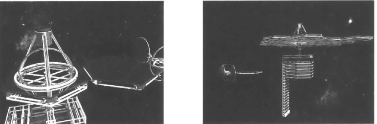
2-9: The total propellant mass is distributed amongst the maneuvers in the way shown ab o v e ... 4 3 2-10: Still shots demonstrating the assembly of a large space structure using EMFF... 45

2-11: Two experim ental EM FF vehicles... 45

2-12: A schematic of the EMFF assembly with the stack of mirrors. This schematic is not to scale, and many components are not included (ex. reaction wheels). ... 46

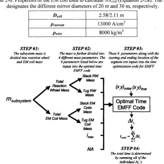
2-13: The algorithm to determine the total assembly time when using EMFF... 47

2-14: The ratio of the times to assemble the telescope for EMFF and propellant... 49

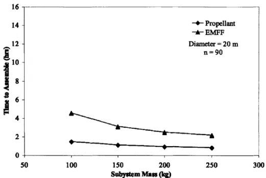
2-15: Comparing propellant and EMFF-based subsystems for a 20-meter telescope with 90 segm en ts... 50

2-16: Comparing propellant and EMFF-based subsystems for a 20-meter telescope with 126 segm ents. ... 50

2-17: Comparing propellant and EMFF-based subsystems for a 30-meter telescope with 90 segm en ts. ... 5 1

(11)

2-18: Comparing propellant and EMFF-based subsystems for a 30-meter telescope with 126 segm ents. ... 5 1

2-19: (a) The maximum acceleration (Equation 2-24) of the segment and (b) the maximum total impulse (Equation 2-26) required by the thrusters for a 20-meter telescope with

90 segm ents. ... 52

3-1: The Gemini 8 docking port (courtesy of NASA). ... 54

3-2: Apollo probe-drogue docking system (courtesy of NASA)... 56

3-3: An example of a spring-loaded latch used with a probe and drogue docking port (courtesy of W igbert Fehse) ... 56

3-4: Spring and damper system used for the probe and drogue docking port... 56

3-5: Russian probe and drogue docking port... 57

3-6: Apollo-Soyuz docking port (courtesy of NASA)... 58

3-7: A "Stewart platform" is used for alignment and shock attenuation (courtesy of W igbert Fehse)... 58

3-8: The Androgynous Peripheral Docking System (APDS) (left). The Androgynous Peripheral Attach System (APAS) (right) (courtesy of RSC Energia)... 59

3-9: A schematic demonstrating a berthing. The grapple mechanism connects to the fixture on the chaser and then docks the two vehicles. ... 59

3-10: The ISS Common Berthing System. This ring is used to rigidly join the two connecting ISS components (courtesy of NASA). ... 59

3-11: DARPA's Orbital Express mission. The two docking spacecraft (a) with a close-up of the grapple/docking mechanism (b) (courtesy of DARPA). ... 60

3-12: Low Impact Docking System (LIDS) (courtesy of NASA)... 61

3-13: Autonomous Satellite Docking System, Developed by Michigan Aerospace (courtesy of M ichigan A erospace)... 61

3-14: Initial misalignment of two docking modules. ... 62

3-15: Large angular articulation of the docking port could be used to connect multiple m o du les. ... 64

(12)

3-17: An example of how the docking port could be used to perform system identification

w ith docked m odules... 65

3-18: Active and passive docking ports ... 66

3-19: Examples of central (left) and peripheral designs (right)... 68

3-20: An example of a reconfigurable docking port design... 68

3-21: An example of an inverse-symmetric docking port design... 69

3-22: Various pin-hole combinations for an inverse-symmetric design... 69

3-23: A CAD drawing of the UDP, showing some of the key features of the design... 71

3-24: Two SPHERES locked together using two UDP's... 72

3-25: The evolution of the UDP. Many different designs were considered. Most of these designs were infeasible due to the complex machining required. ... 73

3-26: Flow-chart showing the docking and undocking sequence... 74

3-27: Input/output structure of the UDP circuit board... 75

3-28: The actual UDP circuit board (right). ... 75

3-29: The pin blocks the sensor. The sensor is mounted directly behind the second rotating ring (Figure 3-30)... 76

3-30: This illustrates how the counter-rotating disks are used to lock the pin. The pin is both pinched and w edged... 78

3-31: The curved slot and pin are used to counter-rotate the disks. ... 78

3-32: The motor is used to move a pin through the curved slots in the disk for counter-rotatio n . ... 7 8 3-33: The routing of the electrical wiring. ... 79

3-34: Attractive force versus axial distance for two active electromagnets... 81

3-35: Attractive force versus axial distance with one active electromagnet, and the repulsive force versus axial distance for two active electromagnets... 81

3-36: Attractive force versus time with near zero separation between the two activated docking ports. ... 82

4-1: T he test setup ... 84

(13)

4-3: The CCD-based camera produces a 2D grayscale image similar to the illustration shown above. The row and column location of the centroid for each LED must be

determ ined (how, h,0I)... 86

4-4: The camera used for the MVDS. The dimensions are 2.5 by 2 inches... 86

4-5: (a) A single LED being imaged on the CCD. (b) Same as (a) but uses the naming convention used in this study. (c) The LED location (Rx,Ry,Rz)1 is converted to a the row and column location on the CCD (how, h,,,). ... 88

4-6: The dimensions that are used to determine the relationship between the LED placement and measurement sensitivity... 89

4-7: Three LED's (left) imaged on the CCD (right). Multiple solutions will exist for particular orientations whenever only three LED's are used. The vertical dashed lines on the right are shown only for reference, and are not part of the actual CCD image. ... 9 0 4-8: Three LED's (far left) imaged on the CCD (far right). The viewpoint of the camera is shown in the center. The image depicts an equal angle change in opposite directions. This is an example of when multiple solutions exist. The vertical dashed lines on the right are shown only for reference, and are not part of the actual CCD image... 91

4-9: Three LED's (far left) imaged on the CCD (far right). The viewpoint of the camera is shown in the center. The image depicts three LED's rotated by an equal angle in opposite directions. Multiple solutions can be eliminated if the center LED is placed out in front in the x-direction. However, this only eliminates the multiple solutions for particular viewpoints. The vertical dashed lines on the right are shown only for reference, and are not part of the actual CCD image... 91

4-10: Determining the center of the LED spot on the CCD... 93

4-11: The algorithm used to find the center of the LED spots on the CCD... 93

4-12: The EKF propagates using the system dynamics and updates using the CCD m easurem ents. ... 94

4-13: A block diagram showing the iterative process of the EKF... 96

4-14: The state of the SPHERE . ... 96

(14)

4-16: The known position of the SPHERE (r) along with the location of the LED's (Si) can

be used to determ ine the R vectors. ... 100

4-17: Flow chart of the M atlab code... 104

4-18: Experimental setup for measuring the MVDS error... 106

4-19: MVDS experimental error (x-direction). ... 107

4-20: M V D S range error (z-direction). ... 107

4-21: M V D S angle error... 107

4-22: The experimental error, which was also shown in Figure 4-19. There is both an error bias (black curve) and an error uncertainty (oscillations)... 110

4-23: The optical model used to explain the error bias term in Figure 4-22. The variables hmeasured and hactual are shown as hm and ha, respectively... 110

4-24: Comparing the experimental error (%) to the theoretical error bias... 111

4-25: Comparing the experimental error to the theoretical error bias... 111

4-26: The optics model used to determine the theoretical uncertainty. ... 113

4-27: Comparing the theoretical and experimental error. ... 114

4-28: The UDP and MVDS hardware used to perform the autonomous docking and undocking tests. ... 115

4-29: The MVDS has an operating range that is defined by a 50 degree full cone... 116

4-30: The distance between the two docking port faces during the docking test... 117

4-31: The relative velocity of the SPHERE during the docking test... 117

4-32: The relative quaternions of the SPHERE during the docking test... 117

4-33: The relative angular velocity of the SPHERE during the docking test... 118

A-1: Bill of Materials (BOM) for the Universal Docking Port. ... 127 C-1: The most general way to specify a rotation of a body in frame T relative to a reference fram e C ... 14 3

(15)

List of Tables

2-1: Some sample commands from the computer to the modules... 30

2-2: The metrics used to determine the relative costs of modularity... 33

2-3: Baseline values for the mirror segments. ... 37

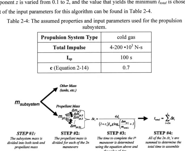
2-4: The assumed properties and input parameters used for the propulsion subsystem... 43

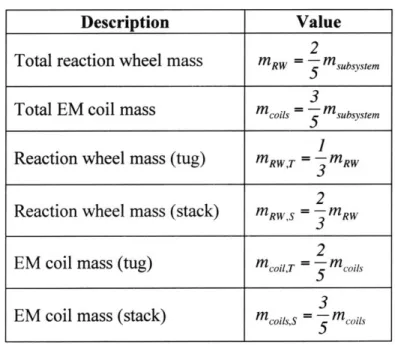
2-5: The masses of the reaction wheels and coils for the tug and stack... 46

2-6: Properties of the EM coil used to calculate NA c 1t (Equation 2-28). The slash designates the different mirror diameters of 20 m and 30 m, respectively... 47

2-7: Input to the EMFF optimal time algorithm... 48

3-1: Key specifications for the UDP... 72

3-2: Sum m ary of U D P Tests ... 80

4-1: The cam era specifications. ... 86

4-2: The values used to determine the theoretical bias and uncertainty error... 114

4-3: The most dominant sources of error for the MVDS. ... 114

4-4: O ther possible sources of error... 115

(16)

Nomenclature

AAR EKF EM EMFF ISS MIT MVDS SPHERES SPHERE SSL SWARM UDP

Autonomous Assembly and Reconfiguration Extended Kalman Filter

Electromagnet

Electromagnetic Formation Flight International Space Station

Massachusetts Institute of Technology Miniature Video Docking Sensor

Synchronized Position Hold Engage and Reorient Experimental Satellites Same as SPHERES

Space Systems Laboratory

Self Assembling Wireless Autonomously Reconfigurable Modules Universal Docking Port

Mathematical Notation

Vectors and matrices are represented in bold italic (e.g. x) Scalars are represented in italics (e.g. x)

AX is a vector X in the A coordinate frame.

Xb is the scalar component of a vector X in the b-coordinate direction. Xis the transpose of X.

(17)

(18)

Chapter 1. Introduction

1.1. Motivation

The exploration of space has continually demanded larger and more complex space systems. The size of such space systems, however, is significantly limited by launch vehicle costs and payload carrying capabilities, while risk management and allowable development time greatly limit the complexity of their design. Thus, it is critical to focus on size and complexity when considering new methods for designing advanced space systems. A modular design methodology would be achieved if a space system were physically divided by separate functions. For instance, a conventional spacecraft consists of multiple subsystems such as propulsion, thermal, attitude control and payload, which are all integrated to form a monolithic system. A modular spacecraft performs the same functions, but each subsystem forms a separate module, which acts independently except through the connections available through one or more standardized interfaces. Using multiple launches, each of these modules could be autonomously assembled with previously launched modules to form a very large system once in space.

A modular space system with the ability to autonomously assemble and reconfigure itself while in space would increase the lifetime of the spacecraft by providing the option of replacing only particular failed subsystems after years of operation. Also, certain system architectures could benefit from the ability to reconfigure. Finally, since each separate module could be designed and tested independently, modularity could reduce the amount of time required for design, manufacturing, integration and testing. Thus, a modular design could be used to increase the size and complexity of a space system.

(19)

1.2. Overview

Chapter 2 presents concepts of modular space systems, and includes definitions and specific examples of how modularity has been incorporated into past and present space missions. In addition, two space system architectures that utilize modularity are presented in more detail to serve as examples of possible applications. Analyses are performed to investigate a few of the first order complexities involved with these particular modular concepts. The first example is a fully modular spacecraft design, which has standardized and reconfigurable components with multiple decoupled subsystems. This concept was developed into a testbed called Self-assembling Wireless Autonomous and Reconfigurable Modules (SWARM), which sought to demonstrate the use of modular spacecraft in a

laboratory environment, and to investigate the "cost," or penalty of modularity.

The second example investigates the on-orbit assembly of a large segmented primary mirror, which is part of a space-based telescope. The objective is to compare two methods for assembling the mirror. The first method uses a propellant-based spacecraft to move the segments from a central stowage stack to a mirror assembly. The second is an electromagnetic-based method that uses superconducting electromagnetic coils as a means of applying force and torque between two assembling vehicles to produce the same results as the propellant-based system. This system is termed Electromagnetic Formation Flight (EMFF). Since only electrical energy, which is abundant through the use of solar panels, is required, the number of maneuvers necessary to assemble the mirror becomes less limited by fuel availability. Moreover, optical contamination due to the exhausts of the thruster-based systems is not an issue with EMFF. Although this telescope is not a completely modular system, it demonstrates the concept of assembling and possibly reconfiguring a large number of modules in space.

The autonomous assembly and reconfiguration (AAR) of any modular space system will involve very complex rendezvous and docking maneuvers, which will certainly require advancements in docking port and sensor technology. To this end, the history of docking ports is presented in Chapter 3, and a comprehensive list of functional requirements is developed. Also, the design and implementation of a universal docking

(20)

port is shown. This docking port has an androgynous design capable of passing mechanical and electrical loads between the connected modules. It is also universal, since any two identical ports can be connected together. Supporting electronics allow for both local and remote computer control of the docking port.

Lastly, Chapter 4 discusses the development of a docking sensor. This optical sensor is called the Miniature Video Docking Sensor (MVDS), and uses a set of infrared LED's, a miniature CCD-based video camera, and an Extended Kalman Filter to determine the six relative degrees of freedom of two docking vehicles. The Synchronized Position Hold Engage and Reorient Experimental Satellites (SPHERES), which were also developed by the MIT Space Systems Laboratory, were used to demonstrate the fully integrated docking port and sensor system. Thus, one of the major objectives of this thesis is to present the general requirements for autonomous docking ports and sensing systems, the design of such systems, and the results from 2-D laboratory experiments.

1.3. Outline

- Section 2.1 discusses general concepts of modularity, and offers examples of how modularity has been incorporated into past and present space missions.

- Section 2.2 presents the development of a ground-based testbed, which sought to demonstrate the use of modular spacecraft in a laboratory environment and to investigate the "cost" of modularity.

" Section 2.3 analyzes two different methods for assembling a large segmented mirror in space as an example of how modularity could be incorporated into spacecraft design.

- _{Section 3.1 briefly describes the history of docking ports and lists docking port} capabilities for unmanned missions where docking is needed to assemble modular space systems.

(21)

e Section 3.4 uses the previously defined docking port capabilities to explain the

design and development of a miniature universal docking port.

e Chapter 4 discusses the development of an optical sensor that provides the relative

state estimation of two vehicles during docking. It discusses the results from ground-based tests, which demonstrated an autonomous docking maneuver using a micro-satellite and the fully integrated docking port and sensing system.

" Chapter 5 summarizes the results from this thesis and offers suggestions for future work.

(22)

Chapter 2. Concepts of Modularity in Spacecraft

Design

A module is defined as an encapsulation of highly interconnected parts, whose external connections are minimized and simple. This chapter will discuss some general concepts of modularity currently being considered and used in spacecraft design. It will also present a brief history of past and present work in the area of modular spacecraft including technology that was developed as part of MIT's modular spacecraft testbed. Lastly, a trade model comparing two different methods for autonomously assembling a modular telescope will be presented.

2.1. Past and Present Work

A modular spacecraft design (MSD) has standardized and reconfigurable components with multiple decoupled subsystems. It also has the ability to reuse these common modules across separate missions. This is in contrast with a common spacecraft design (CSD), which involves using identical but non-reconfigurable designs, or a heritage spacecraft design (HSD), which is heavily based upon previous designs. A modular spacecraft design holds promise for reducing the amount of time required for design, manufacturing, integration and testing.

The commercial, military and science communities would directly benefit from modular designs by having the option of replacing only particular subsystems of a spacecraft. For example, a failed propulsion subsystem could be replaced on orbit instead of the entire spacecraft. Another benefit of a modular design is the ability to launch large spacecraft using one or more launches. Once in space, the modules could be autonomously deployed and assembled. The spacecraft could then be reconfigured to accommodate various mission objectives. Lastly, standardization gives rise to compatibility across

(23)

organizations and allows for more domestic and international collaboration. As space technology advances, there is a need for standardization and modularity if space technology is to follow a similar path as other successfully advanced technologies such as automobiles, aircraft and electronics.

However, the major drawback with a modular spacecraft design is the need for each subsystem to function independently except through the connections available through one or more interfaces (docking ports). Because of this, the modular design will most likely be sub-optimal and performance may be sacrificed.

Past Work

An early pioneer of a common and heritage spacecraft designs was the Multi-mission Modular Spacecraft (MMS), which was developed by NASA's Goddard Space Flight Center [1]. The MMS was established in the 1970s, and consisted of the following earth-orbiting missions:

e Landsat 4 and 5

e The Ocean Topography Experiment (TOPEX/Poseidon)

* Upper Atmospheric Research Satellite (UARS)

e Extreme Ultraviolet Explorer (EUVE) e Solar Maximum Mission (SMM)

The MMS was part of NASA's pre-Challenger-disaster vision for satellite servicing. The MMS had the following modules:

e Propulsion

e Power

* Attitude control

- Command and data handling

e Other sub-modules to provide signal conditioning and support for an Earth horizon

(24)

Mariner Mark II was NASA's planned family of unmanned spacecraft for the exploration of the outer solar system that were to be developed and operated by NASA's Jet Propulsion Laboratory between 1990 and 2010. Mariner Mark II was intended to be the deep space version of the MMS, which was proven to be very successful for earth orbital missions. Using the same concepts of a standard bus and modular equipment, JPL hoped to cut mission costs in half [2].

The first two Mariner Mark II applications were to be a mission to Saturn and its moon Titan, the Saturn Orbiter/Titan Probe, or SOTP (later called Cassini) and the Comet Rendezvous Asteroid Flyby, or CRAF. Congress approved both of these missions in 1990. Other planned Mariner Mark II based spacecraft included the European mission called the Comet Nucleus Sample Return or CNSR (later Rosetta). However, Congressionally imposed budget cuts forced NASA to terminate the CRAF mission and to delay the Cassini launch. They were also forced to significantly redesign Cassini to reduce the total program cost, mass and power requirements. In essence, the spirit of Mariner Mark II, and the use of modular spacecraft for deep space were terminated due to budget cuts. This shows that the upfront cost of modularity makes it very susceptible to budget cuts when short-term savings drives decisions.

Present Work

Much of the present work focuses on defining the capabilities and major complexities with designing modular spacecraft. The complexity of modular designs largely depends on the capabilities and quantity of docking ports required for a particular mission. A trade was done by Moynahan and Touhy [3], which concluded that the docking port for a modular spacecraft should provide the following connections between modules:

* Data/communication * Mechanical

* Electrical

They also concluded that the thermal system should be left as a function for each individual module to manage, and thus should not be part of the docking port. This issue of

(25)

defining the actual interface between modules is difficult, and would likely be reconsidered for each mission.

More recent effort to develop concepts of modularity in spacecraft design include the following projects and missions:

Name: Small, Smart Spacecraft for Observation and Utility Tasks (SCOUT) Collaborators: DARPA, Aero/Astro Inc.

Description: A multi-mission, rapidly configurable micro-satellite to enable responsive deployment of tactical capability to orbit [4].

Name: The Flexible and Extensible Bus for Small Satellite (FEBSS) Collaborators: Air Force Research Laboratory, Aero/Astro Inc. Description: A low-cost, modular bus for small satellites [4].

Name: Panel Extension Satellite (PESAT) Collaborators: University of Tokyo

Description: A satellite made of several functional panels, including a computer, battery, communication, attitude control and thruster panels. Panels are connected in a "plug-in" fashion, and the total integrated system acts as a conventional satellite. The panels will be stowed during launch within a small volume and then extended on orbit with hinge and latch mechanisms [5].

To summarize, modular technology was successfully demonstrated in MMS missions, though it has been removed from some subsequent missions due to budget cuts. Most of the present work focuses on the interfaces between modules, and how the modules should be integrated to form a complete system. The next section will discuss the modular spacecraft technology that was developed as part of the SWARM project.

(26)

2.2. Modular Technology Development with SWARM

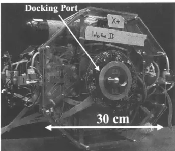
SWARM stands for Self-assembling Wireless Autonomous and Reconfigurable Modules (Figure 2-1). The project sought to demonstrate the use of modular spacecraft in a laboratory environment, and to investigate the "cost," or penalty of modularity. While the lab prototypes closely resemble an actual space system, they were not designed for the space environment. The SWARM system consists of the following separate modules (the quantity is in parenthesis):

- Computer (1)

e Attitude Control System (ACS) (1)

* Propulsion (2) " Mothership (1)

Each module performs a set of subsystem functions and is supported by the following common components (the quantity is in parenthesis):

e Structural package/containment (1)

- Power supply and distribution bus (1)

* Bluetooth chip for wireless command and data handling (1) Field programmable gate array (computer) (1)

* Metrology sensors (4 sets) Docking port (up to 4)

The computer module is the central processor, and gives commands wirelessly to the local computer on each module using the standard Bluetooth@ protocol. A laptop is currently used as the computer module. By using wireless communication, the modules are able to communicate in both docked and formation flown architectures. The ACS module provides rotational torque and is capable of storing angular momentum for the entire spacecraft. This module is essentially a motorized flywheel with a gyro and

(27)

microprocessor that are used to perform all local sensing and low-level commands. The ACS module receives a commanded change in angle from the computer module, and by integrating the on-board rate gyro, executes the command by applying torque against the flywheel. The propulsion module provides the thrust for rotation and translation. Each propulsion module has a firing circuit and six thrusters, which use a supply tank of liquid CO2 and a pressure regulator. This module converts thrust commands into a series of firing

circuit on-times via a pulse width modulation scheme. The Mothership module acts as a much larger vehicle that provides electrical power for charging. It is essentially a rigid post with all of the common components previously mentioned except for the structural packaging. The Mothership is connected to a wall outlet, which provides a continual supply of electrical power for charging once the modules are docked.

The ACS and propulsion modules are mounted on air-carriages and float on a flat surface (Figure 2-2). For simplicity, the Mothership and computer modules are stationary and not contained within the standard module packaging.

As previously stated, a module is defined as an encapsulation of highly interconnected parts, whose external connections are minimized and simple. For SWARM, the structural packaging is the encapsulation, while the docking port and Bluetooth provide the simple external connections.

Docking

Port-<-30 cm

Figure 2-1: A SWARM Module with a docking port. The metrology sensors are mounted around the docking port.

(28)

SPHERE ni

Docking Port Pairs

Propulsion ACS Propulsion

Module _n Module _n Module_n

... ~75

cm

----...-Figure 2-2: A SPHERE [6], two propulsion modules and an ACS module, sitting on air-carriages and rigidly connected using the docking port.

2.2.1. Overview of the docking port

The docking port is a critical piece of the SWARM design. Each module must function independently except through the connections available through this interface and the Bluetooth communication. The SWARM docking port must be capable of performing the following functions between each module:

* Autonomously Dock/Undock: This provides the ability for the modules to be assembled and reconfigured without human intervention.

e Transfer Mechanical Loads: By mechanically connecting the modules, separate

propulsion and ACS modules are able to control the translation and rotation of the entire module cluster.

* Transfer Electrical Power: This allows the modules to share electrical power. For example, the Mothership can charge the other modules.

(29)

e Provide a Connection for Data and Communication: Communication between

modules is necessary for docking/undocking, transferring range data, and general system control.

Section 3.4 will give a detailed description of the SWARM docking port.

2.2.2. Wireless communication using Bluetooth

SWARM uses wireless communication because it offers many practical advantages when compared to a wired system [7]. Wireless communication is inherently complementary to a modular system, since it provides a communication link between separated modules. System-level integration and reconfiguration of the modules will be easier by eliminating the need for a wired connection between docking ports. Also, wireless communication removes mass while increasing the available volumetric space by eliminating the presence of physical wiring. Lastly, it provides real-time communication, and reduces electromagnetic interference (EMI) by eliminating some of the EMI-producing components. However, wireless technology is still under development for space applications, and there are clear disadvantages to choosing this option. For example, radiation in the space environment could cause interference with wireless data transmission. Also, wireless communication generates electromagnetic radiation (EMR). This could be a potential problem for sensitive payloads that are susceptible to this form of radiation. There is also a chance that wireless communication will produce higher development costs due to the complexity of the hardware and software.

Bluetooth is the wireless communications system chosen for SWARM, mainly because of its low cost and standardized architecture. A Bluetooth chip is on the common circuit board, of which every module has identical copies. This chip is the BR-SC 1 A 18-pin STAMP module from Blueradios [8]. This was chosen because of its low cost ($50 per chip) as well as low power consumption (0.35W). The main computer uses a Bluetooth USB dongle to communicate on the SWARM network. The dongle contains the same basic chip but with a modified enclosure and connection interface.

(30)

All of the communication is routed through the main computer module, which forms a master-slave architecture. This takes advantage of the piconet structure of Bluetooth. A piconet is defined as a single master and up to 7 slaves, which is sufficient for the initial SWARM testing. However, future modular systems will likely require more slave modules, and thus Bluetooth's scatternets structure will be required. Scatternets are combinations of piconets joined through one or more slave modules existing in both networks. This would allow additional "parked" slaves to exist in a low-power consumption mode for increased overall network size. According to Bluetooth

specifications, up to 255 "parked" slaves could be on the scatternet [9].

One of the biggest challenges in implementing a wireless network is the error checking and correction. The difficulty is caused by bit corruption in the wireless network, which is mainly caused by radio interference. Bluetooth minimizes this interference by using a built-in spread-spectrum frequency error checking technique. This technique synchronizes up to 1600 hops per second between communicating master and slave modules. This significantly reduces the amount of interference encountered by the transmissions. Bluetooth also employs a variable system of data packet checking and reception acknowledgement to ensure accurate data transmission. Depending on the configuration used for a transmission as well as the level of outside interference, the error-checking system could influence the maximum achievable bandwidth. There are three kinds of error correction schemes used in the baseband protocol of Bluetooth: 1/3-rate Forward Error Correction (FEC), 2/3-rate FEC and Acknowledgement Request Repeat (ARQ) configuration. In 1/3-rate FEC, every bit is repeated three times for redundancy. In 2/3-rate FEC, a generator polynomial is used to encode 10-bit code to a 15-bit code. In the ARQ configuration, DM (Medium-Rate Data) and DH (High-Rate Data) packets are retransmitted until an acknowledgement is received (or timeout is exceeded). Automatic Repeat reQuest Numbers (AQRN) are used as a 1-bit acknowledgement indication to inform the source of a successful transfer of payload data with cyclic redundancy checking. Bluetooth uses fast, unnumbered acknowledgement in which it uses positive and negative acknowledgements by setting appropriate ARQ values. If the timeout value is exceeded, Bluetooth flushes the packet and proceeds with the next.

(31)

A very important component of the wireless system is the protocol used for communication between the computer and any other module. This protocol must include all necessary commands for system operation as well as the data structure that will contain the relevant information. Each transmission to or from the computer module will have both header and data bytes. This form only includes the information being sent to or from the computer. All the error checking is part of the internal header structure and is handled entirely by Bluetooth. Each of the present headers contains three bytes of information consisting of the following items:

e 3-bit Origin ID: Source of the transmission

* 3-bit Destination ID: Desired destination of the transmission

e 4-bit Command: Value of the command being sent to the destination module

* 10-bit Data Length: Number of bytes contained in the data portion of the transmission

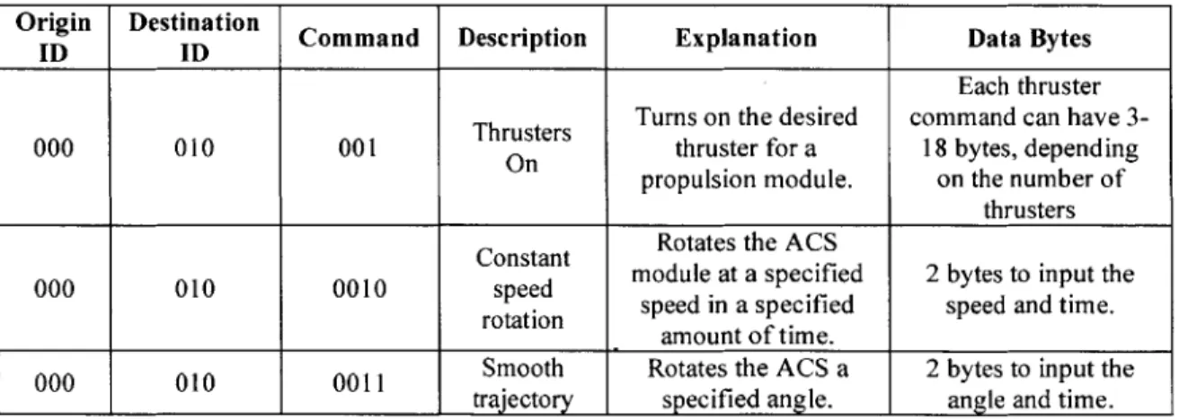
The data portion of the transmission will contain the information for the actual command. Currently, each communications packet can contain up to 1023 bytes of information. Table 2-1 contains a few examples of commands from the computer to the modules.

Table 2-1: Some sample commands from the computer to the modules. Origin Destination Command Description Explanation _{Data Bytes}

ID ID

Each thruster Thrusters Turns on the desired command can have

3-000 010 001 On thruster for a 18 bytes, depending

propulsion module. on the number of thrusters

Constant Rotates the ACS

000 010 0010 speed module at a specified 2 bytes to input the rotation speed in a specified speed and time.

amount of time.

000 010 0011 Smooth Rotates the ACS a 2 bytes to input the

trajectory specified angle. angle and time.

Most of this information on wireless communication was taken from the SWARM design document [7].

(32)

2.2.3. Determining the cost of modularity

If the actual "cost" of modularity is well understood in terms of metrics such as mass and development costs, then a modular design could be successfully implemented for missions that would benefit from such a design. However, determining the absolute cost of modularity is very difficult. Enright, Jilla and Miller [10] sought to determine mission scenarios for when a modular design might be appropriate based on possible cost savings, when compared with an equivalent non-modular design. They concluded that modularity could offer cost savings for missions involving a small number of satellites when the design is driving the mission cost. However, as the mission size increases, the mass and launch costs increase greatly. Thus a lighter custom (non-modular) design may yield better price performance. They also concluded that modular designs in two ranges of mission size offer large savings when production costs are dominant. The first region covers very small missions (few satellites), where the initial learning curve savings are dominant. The second includes modest sized missions (about a dozen spacecraft), where the design and secondary learning curves savings allow large savings (regions with high learning curve factors). Thus, they concluded that the size and complexity of the mission largely dictate the cost savings of modularity.

Instead of determining whether or not modularity is appropriate for a given mission, SWARM was analyzed to determine the relative cost of modularity. This is a qualitative measure of the penalty induced by having a modular design. The relative cost determines which components most heavily penalized the design by adding size, mass and complexity. The common components in SWARM were grouped together and rated based on a set of penalty metrics. The following groups of components were considered:

1. Structural packaging: The additional packaging that is required to separate the various subsystems into their own structurally rigid containment. It is the "encapsulation," which is part of the definition of a module as previously stated. In the case of SWARM, this is the metal structure used to enclose the propulsion and ACS modules.

(33)

2. Docking port and sensors: The docking port is the only physical connection between modules. The sensors allow the modules to dock and undock for reconfiguration maneuvers.

3. Electronics/cabling: All the electronic components that are common among modules. This includes the FPGA, power distribution card and Bluetooth chip, and all the necessary cables.

The following penalty metrics were used to rate each of the groups:

1. Volume: Measures the volumetric space occupied by the component. Components that occupy a large volume are penalized with a high rating.

2. Mass: Measures the significance of the mass added by this group. If the mass is relatively significant, then it is penalized with a high rating.

3. Complexity: Measures the added complexity in the spacecraft design by having this component. If the component was very complex to design, then it is penalized with a high rating.

4. Non-scalability: Measures the scalability of the group. Can it be shrunk in size for smaller modules and increased in size for larger modules? If the component cannot be easily scaled, this is bad for modularity and thus is penalized with a high non-scalability rating.

Each group is given a relative metric rating from 1 to 3 (1 = low, 3 = high). Each metric has a "weight" based on its significance to the overall design. The results of this analysis can be found in Table 2-2.

(34)

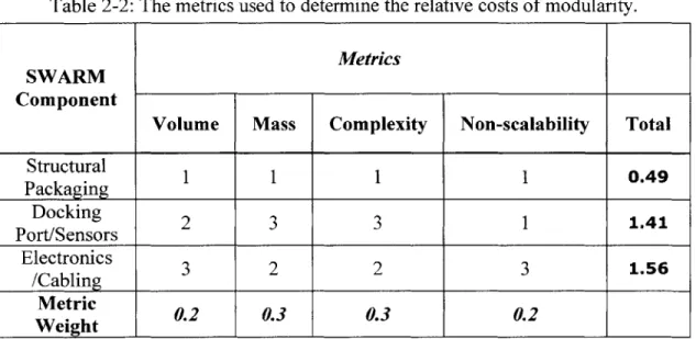
Table 2-2: The metrics used to determine the relative costs of modularity.

Metrics

SWARM Component

Volume Mass Complexity Non-scalability Total Structural Packaging Docking 2 3 3 1 1.41 Port/Sensors Electronics 3 2 2 3 1.56 /Cabling Metric _0.2 _0.3 _0.3 0.2 Weight 0 0 0 0I2

The key result from this analysis is that the electronics were the most costly component. This result can be confirmed by viewing the inside of the module; most of the complexity and volumetric space constraints are caused by the electronics. The electronics were given a high non-scalability score because it is difficult to shrink the electronics for small modules like SWARM. However, it should be noted that the size of the electronics would remain approximately the same size for a module three to four times the size of SWARM. Thus, for large modules the electronics may be less of an issue, while the larger docking port may become more significant.

2.3. A Trade Model for Assembling a Large Space Telescope

There is current interest in the ability to assemble large systems in space. An example is DARPA's LASSO program, which will examine the feasibility of manufacturing a large optical structure in space. The proposed LASSO system is a 150-meter optical system in geosynchronous orbit [11]. This section investigates the on-orbit assembly of a large segmented primary mirror, which is part of a space-based telescope. The concepts developed in this section are very general, and could be applied to other scenarios such as the proposed LASSO system. It has been assumed that large mirrors (-20 meters) will be assembled in space using a stack of hexagon-shaped mirror segments. The

(35)

objective is to compare two methods for assembling the mirror. The first method uses a propellant-based tug spacecraft to move the segments from a central stowage stack to the mirror assembly. The second is an electromagnetic-based method that uses superconducting electromagnetic coils as a means of applying force and torque between two assembling vehicles to produce the same results as the propellant-based system. This system is termed Electromagnetic Formation Flight (EMFF) [12].

Metrics are required to compare these two methods. Usually cost is the metric chosen to make this type of comparison; the configuration that achieves the same level of performance for a lower cost is chosen. However, cost is directly proportional to mass for many space systems, thus mass is the metric analyzed in this report.

2.3.1. Problem definition and scope

Each segment is stowed in a vertical stack as shown in Figure 2-3-a. The tug begins at the top of the stack, and delivers each segment to the predetermined location in the primary mirror and then returns to the next segment in the stack. The mirror is assembled according to the numbering sequence shown in Figure 2-4. The size of the mirror and number of segments is a parameter that can be varied. The following items are not considered in this study:

- Space effects: Orbital dynamics and solar pressure.

e Removal and installation processes: Rotation and reorientation of the mirror

while taking it from the stack and then just before attaching it to the mirror assembly. Also, the time to dock and connect the mirrors together.

* Optimal trajectory planning / collision avoidance: Certain delivery and return paths of the tug may be suboptimal, and alternative trajectories may be required to avoid collision with other segments. Also, issues such as optical contamination due to propellant plumes are not considered.

* Optimal stacking configurations: It may be more optimal to assemble the mirror using a horizontal stack rather than the vertical stack used for this study.

(36)

- Imperfections in the control system: The thrusters and EMFF subsystems may not perform perfectly at all times.

e Optimal fuel usage: There may be more globally optimal solutions for managing

the propellant.

* Larger trade space: Only 20 and 30-meter diameter telescopes are considered. Large diameters could be explored.

-5--10 -15 -20 -25 -30 -10~ 0 10 15 -10 ~ 0 ~ 1 (a) 0, -5, -10, -15, -20s -25, -30 10 0 20 10 -10 0 -10 -20 + + +++ + +-.+ 4. 0- + + + + + -5- + -10- -15- -20- -25--30- 10 0 -10 _-10 00 20 (b) 0 -5 -10 -16 -20 -25 -M0 -.36 20 10 0 -10 -200 -20 -10 10 2 (c) (d)

Figure 2-3: The segments start in a stack (a). The delivery point for each segment is predetermined and is represented as points (b). An optimal trajectory is chosen (c) and

(37)

Figure 2-4: The assembling starts with number one and continues clockwise following the numbering sequence shown above.

2.3.2. Sizing the mirror segments and tug vehicle

The diameter of the mirror, D, and the number of segments, n, must be initially specified. The effective area of the mirror, A, can be determined using:

icD

2

Ae= 2-1

4 Thus the area of an individual segment, A,, is:

A= Ae 2-2

n

Where n is the number of segments. The side length of the hexagon can be determined using the known segment area (Figure 2-5):

2

s A 2-3

Now that s is known, the center of the hexagon for each segment can be determined as shown in Figure 2-3-b.

The mass of an individual segment can be determined by assuming a known areal density of the mirror (Pareat). It will be assumed that the areal density includes the glass, coating, structural supports, and docking ports (Figure 2-5). Thus the mass of a single segment, msegment, is then:

(38)

The hexagonal mirror segments currently being used on the Keck telescopes will be used to approximate the size and mass of the mirror segments used in this study. The areal density for the Keck mirrors is approximately 190 kg/M2_{, which includes the mass of the}

glass, supporting structures and actuators. Since much less mass would be required in a zero-g environment, it will be assumed that an advanced space version would be approximately 90% lighter. A 20 and 30-meter telescope with 60 segments and another with 90 segments will be considered in this study. A complete list of the baseline values for the 20-meter telescope is shown in Table 2-3.

Table 2-3: Baseline values for the mirror segments.

Keck Space Telescope

(approx. values) (assumed values)

Effective diameter of the 10m _{20 m}

primary mirror

Effective area of the 78 m2

314 m2

primary mirror

Number of segments 36 60/90

Area of a single segment 2.11 m2 _{5.24/3.5 m}2

Size of a hexagon _{0.9 m} _{1.42/1.16 m}

segment (s)

Areal density 190 kg/m2 _{20 kg/M}2

Mass of a single segment 400 kg 104/70 kg

Mass of all segments 14400 kg 6300 kg

Length of stack NA 15/22.5 m Single Mirror Segment Docking Port Structural Supports

Front of Mirror Back of Mirror

Segment Segment

(39)

The mass of the tug, miug can be determined by assuming that:

m =2msegment 2-5

This would put the center of mass for the combined system inside the volumetric space of the tug vehicle, which may be desirable for control purposes. The mass of the tug is a dry mass and does not include the propellant or EMFF components. The propellant components are the thrusters, tanks and fuel. The EMFF components are the electromagnet coils and reaction wheels. The cargo mass, mcargo, is defined as:

cargo = segment tug 2-6

It should be noted that the segment mass is only included in mcargo when the tug is delivering a segment to be assembled. On the return trip to the stack the segment mass is not included. Also, the total mass, mtota,, is defined as:

mtotal =m cargo + subsystem 2-7

where the subsystem mass, msubsystem, is a summation of the propellant and EMFF-specific components such as thrusters, tanks, coils and reaction wheels. The next two sections discuss the individual propellant and EMFF subsystems. It will be shown that the total time to assemble, ttotal, can be determined for a specified amount of subsystem mass.

2.3.3. Propellant-based subsystem

The objective of this section is to determine the total time required to assemble the mirror assembly when the propellant-based subsystem is used. It will be shown that the total time to assemble the mirror can be determined if the subsystem mass, msubsystem, is specified. The propellant-based tug was modeled as a spacecraft with eight sets of 3-axis thrusters (Figure 2-6). A "blowdown system" will be assumed, which uses the initial pressure inside its tanks to expel propellants. Thus it will be assumed that no electrical power is needed to generate thrust [13].

Besides the expelled propellant mass, there are many other components that add mass to the propellant-based system. Typically the tank mass, mtank, can be estimated as

(40)

15% of the propellant mass, and the mounting hardware and propellant management devices, mH/w, are an additional 30% of the tank mass [13]. Also, each thruster has a mass,

mth. These assumptions can be used to determine the subsystem mass:

Msubsystem M tan + + Nthmth + MH/W 2-8

= m,, + 0.15m,, + Nthmh + .3 mtank 2-9

= Mp, + 0.15m,, + Nth mh + 0.3(0.15)mpt 2-10 Thus, the total subsystem mass for the propellant components can be estimated using:

msubsstem .2mp,+ Nhmth 2-11

where m,, is the total mass of the propellant and Nh is the number of thrusters. The dry mass of the propellant system, m,,d,, is defined as:

pt,dry subsystem ~ pt 2-12

Port used to

grapple mirror

Thrusters

Figure 2-6: The "tug" used to assemble the mirror for the propellant-based subsystem.

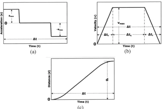
The temporal profiles for the thrusters are shown in Figure 2-7, and can be used to determine the mass of the propellant.

(41)

--Time (t) 0Tm t

(a) (b)

0 _me

(c)

Figure 2-7: Temporal profiles for a single maneuver.

From Figure 2-7, it can be shown that the total change in velocity for a single maneuver is:

AVj = 2v, .= 'd 2-13

Ati(1I t

where vm,,,i is the maximum velocity (Figure 2-7-c), di and Ati are the distance and time respectively for the i'th maneuver, and ci is defined below. A maneuver is defined as either a single delivery of a segment, or a return trip of the tug to the stack. Thus, two maneuvers are required to assemble a single segment. The distance traveled during each maneuver (di) is predefined for each maneuver based on the known geometry and predetermined path. For the propellant case, the optimal path is a straight line between the starting and ending point of each maneuver (Figure 2-3-c). The variable ci in Equation 2-13 is defined as:

Atr4 t

.4

c. = At2 2-14

'.Ati

where At,, iTs the amount of time the tug coasts without firing the thrusters (Figure 2-7-b). Thus, the value of ci is the fraction of time the vehicle coasts during each maneuver, and can be varied from zero to one. It can be seen from Equation 2-13 that A V is minimum

(42)

when c, equals unity, for a fixed distance and time. However, as ci approaches unity the acceleration becomes infinite, and as it approaches zero the thrusters near a "bang-bang"

firing profile. Thus, a reasonable value of ci can be chosen based on the limitations of the thrusters.

The "Rocket Equation" relates the A Vi to the propellant fuel required for each maneuver, Jmpt i(Appendix B): =mt :-Mtot0 ₁₁j e ' - 2-15 where VI 2-16 where Ve is the exhaust velocity of the propellant and g is the gravitational constant at sea level. The total mass, motali, is the mass being moved by the tug during the ith maneuver, which includes the cargo mass, the fuel mass required to complete all of the 2n-] future maneuvers, and the dry mass of the thrusters and tanks:

mol,= m argo, + m P, + mpdr, 2-17

j=2n

Note that in Equation 2-17 the summation starts at the very last (j 2n) maneuver, and sums backwards to the present (jih) maneuver. This is because the total mass must also include the propellant required for all of the future maneuvers. Thus, the first maneuver has to carry all the fuel required to perform the single maneuver plus all the remaining maneuvers. The algorithm for determining the total assembly time for the propellant subsystem is summarized in Figure 2-8. By combining Equations 2-13 and 2-15, the time required for each maneuver can be determined:

4d.

At. = I ')