The tails of the satellite auroral footprints at Jupiter
B. Bonfond1 , J. Saur2 , D. Grodent1 , S. V. Badman3 , D. Bisikalo4, V. Shematovich4, J.-C. Gérard1 , and A. Radioti1
1Space sciences, Technologies and Astrophysics Research Institute, LPAP, Université de Liège, Liège, Belgium,2Institut für
Geophysik und Meteorologie, Universität zu Köln, Cologne, Germany,3Department of Physics, Lancaster University,
Lancaster, UK,4Institute of Astronomy, Russian Academy of Sciences, Moscow, Russia
Abstract
The electromagnetic interaction between Io, Europa, and Ganymede and the rotating plasma that surrounds Jupiter has a signature in the aurora of the planet. This signature, called the satellite footprint, takes the form of a series of spots located slightly downstream of the feet of the field lines passing through the moon under consideration. In the case of Io, these spots are also followed by an extended tail in the downstream direction relative to the plasma flow encountering the moon. A few examples of a tail for the Europa footprint have also been reported in the northern hemisphere. Here we present a simplified Alfvénic model for footprint tails and simulations of vertical brightness profiles for various electron distributions, which favor such a model over quasi-static models. We also report here additional cases of Europa footprint tails, in both hemispheres, even though such detections are rare and difficult. Furthermore, we show that the Ganymede footprint can also be followed by a similar tail. Finally, we present a case of a 320∘ long Io footprint tail, while other cases in similar configurations do not display such a length.1. Introduction
Among the many features of the Jovian aurora (see review by Grodent [2015]), the satellite footprints of Io, Europa, and Ganymede are some of the most easily recognizable ones [Connerney et al., 1993; Clarke et al., 2002]. In a reference frame fixed with the Jovian magnetic field, called System III (SIII), they have a very
dis-tinctive motion since they are fixed with their respective satellite rather than rotating with Jupiter or fixed with local time. Enceladus also leaves an auroral footprint on Saturn [Pryor et al., 2011]. The footprint of Io is made of at least three spots and an elongated tail [Connerney and Satoh, 2000; Clarke et al., 2002; Gérard et al., 2006; Bonfond et al., 2008, 2009]. The Ganymede footprint and, on rare occasions, the Europa footprint (EFP) also display at least two spots [Bonfond et al., 2013a, 2017]. The relative distance between these spots varies in a systematic way with respect to the SIIIlongitude of the satellite, which provides precious clues about the
mechanisms at play.
These three satellite footprints arise from the electromagnetic interaction between the satellites and the rapidly rotating magnetospheric plasma, which generates Alfvén waves propagating along the magnetic field lines [e.g., Saur, 2004]. These waves can be partially reflected on the density gradients at the plasma torus/plasma sheet boundaries [Neubauer, 1980; Goertz, 1980]. At high latitude, dispersive effects become sig-nificant and the Alfvén waves develop an oscillating electric field along the field lines, accelerating electrons both toward the planet and in the opposite direction [Jones and Su, 2008; Hess et al., 2010, 2013]. The electrons moving planetward will generate an auroral feature called the main Alfvén wing (MAW) spot. The others will create a Trans-hemispheric Electron Beam (TEB) spot in the opposite hemisphere [Bonfond et al., 2008]. The waves that were reflected once against a plasma torus/sheet boundary can still be partially transmitted through the opposite boundary and give rise to a Reflected Alfvén Wing (RAW) spot. Because multiple spots are also observed for the Europa and the Ganymede footprints [Bonfond et al., 2013a, 2017], the idea that these processes are common to all footprints is consistent with the data. Grodent et al. [2006] showed evidence for a Europa footprint (EFP) tail, based on three sets of images of the northern aurorae acquired by the Hubble Space Telescope in 2005. These authors suggested a possible relationship between the Europa footprint tail and the extended plasma plume observed downstream of Europa [Eviatar and Paranicas, 2005]. This plume arises from the interaction between Europa’s atmosphere and the magnetospheric plasma, which could be enhanced as Europa encounters the denser central plasma sheet [Kivelson et al., 1999]. However, the interac-tion at Ganymede is very different because the obstacle to the plasma flow is the whole mini-magnetosphere
RESEARCH ARTICLE
10.1002/2017JA024370
Key Points:
• The length of the footprint tail is not a reliable parameter to differentiate quasi-static and Afvénic tail generation models • Monte Carlo simulations favor
the Alfvénic electron acceleration scenario over the quasi-static electric field scenario for the tail • The Europa and Ganymede footprints
also have a tail, in both hemispheres
Supporting Information: • Supporting Information S1 • Figure S1 • Figure S2 • Data Set S1 • Data Set S2 • Data Set S3 • Data Set S4 • Data Set S5 • Data Set S6 • Data Set S7 • Data Set S8 • Data Set S9 • Data Set S10 • Data Set S11 • Data Set S12 • Data Set S13 • Data Set S14 Correspondence to: B. Bonfond, [email protected] Citation:
Bonfond, B., J. Saur, D. Grodent, S. V. Badman, D. Bisikalo, V. Shematovich, J.-C. Gérard, and A. Radioti (2017), The tails of the satellite auroral footprints at Jupiter, J. Geophys. Res. Space Physics, 122, doi:10.1002/2017JA024370.
Received 16 MAY 2017 Accepted 7 JUL 2017
Accepted article online 19 JUL 2017
©2017. American Geophysical Union. All Rights Reserved.
Table 1. List of the Relevant Parameters to Compute the Length of the Footprint Tails According to the Model of Hill and Vasyli¯unas [2002]a
Parameter Io Europa Ganymede
Equatorial volume mass density (amu cm−3)𝜌
ea 64,300 3,000 100
Equatorial magnetic field strength (nT)Bea 1,720 370 64 Relative plasma velocity (km s−1)𝜈
0a 57 76 139
Distance from Jupiter (km)Db 421,800 671,100 1,070,400 aThese numbers come from Kivelson et al. [2004].
bThese numbers come from Weiss [2004].
of Ganymede [Paty et al., 2008; Jia et al., 2009a; Saur et al., 2013; Duling et al., 2014]. Moreover, this magnetic field at least partially shields the atmosphere of Ganymede, and there likely is much less mass loading than at Io or Europa.
Most theoretical models of the Io footprint (IFP) tail emission [Hill and Vasyli¯unas, 2002; Delamere et al., 2003; Su et al., 2003; Ergun et al., 2006; Matsuda et al., 2012] assume that it is caused by the acceleration of quasi-stagnant plasma in Io’s rest frame, i.e., from the orbital speed of Io, to corotation with Jupiter. In these models, the plasma is accelerated by j × B forces, where the electric current is continued as field-aligned current into the ionosphere of Jupiter from which the momentum is exerted. A consequence of these currents is the for-mation of a quasi-static electric potential above the planetary ionosphere which accelerates electrons toward Jupiter’s atmosphere, thus creating the IFP tail. In this scenario, the IFP spots and the tail would be created by two different mechanisms: an Alfvénic one for the spots and a steady one for the tail.
In section 2, we explore another scenario, in which the interaction remains Alfvénic all along the tail and we show that the two model families predict similar tail lengths. Such an Alfvénic scenario explains very naturally why observations of the brightness vertical profile in the tail shows no difference with the MAW spot profile [Bonfond, 2010]. On the other hand, two different mechanisms have been proposed to explain this similarity even if the tail was produced by a steady process [Matsuda et al., 2012]. However, we show simulation results indicating that neither of them could actually reproduce the observations (section 3). If the nature of the IFP tail is Alfvénic, with only a small amount of momentum loading arising from mass loading relative to the total momentum exchange of the interaction, then all three footprints on Jupiter could also have a tail, which we demonstrate in section 4.
2. Analytical Estimations for the Footprint Tail Length
The good agreement between theory and observation concerning the IFP tail length has often been used as an argument in favor of the quasi-static acceleration models. Indeed, using a set of parameters adequate for the Io case, Hill and Vasyli¯unas [2002, HV] showed that their model predicts a length scale (e-folding distance) 𝜑0= ∼ 12∘, in accordance with direct observations of the brightness profile from the Hubble Space Tele-scope [Clarke et al., 2002]. With updated parameters (see Table 1), the same model predicts values around 20∘. It should, however, be noted that measurements of the typical e-folding distance based on observations of the IFP tail above the limb provided values ∼21, 000 km, corresponding to ∼40∘ of longitude [Bonfond et al., 2009]. It can thus be concluded that the theory and observations agree within a factor of 2.
The same model could be used to estimate the Europa footprint (EFP) and Ganymede footprint (GFP) tails’ lengths, since it predicts that the length scale depends on the velocity of the ambient plasma relative to the moon𝜈0, the equatorial mass density𝜌e, the thickness H of the plasma sheet in one hemisphere, Jupiter’s
height-integrated Pedersen conductivity Σ, the equatorial magnetic field strength Be, and the distance to
Jupiter D: 𝜑HV 0 = 𝜈0𝜌eH 2ΣB2 eD . (1)
If we assume, contrary to the Io case where extensive ion pickup is taking place, that the density of the ini-tially stagnant flux is similar to the surrounding density since less mass loading is expected at Europa and Ganymede compared to Io, then, using the values reported in Table 1,𝜑Europa0 ≈ 6∘ and𝜑Ganymede0 ≈ 11∘.
If the footprint tails are generated by such a quasi-static process while the spots are related to dispersive Alfvén waves, then the energy distribution of the precipitating electron population would be expected to be quasi-monoenergetic in the tails and broader in the spots. Such a discrepancy between narrow distributions associated to inverted-Vs and broader distributions related to Alfvén waves are frequently observed at Earth [e.g., Paschmann et al., 2002; Motoba and Hirahara, 2016]. However, in the IFP case, observations of the vertical brightness profile show a similar and broad distribution for both the main spot and the tail [Bonfond et al., 2009; Bonfond, 2010]. An alternative scenario, consistent with MHD simulations of the Alfvén waves’ propa-gation [Jacobsen et al., 2007, 2010], is that the spots and the tail all arise from the same Alfvénic process as the Alvén waves continue to bounce downstream relative to Io.
In the Alfvénic picture a simple model for the length of the tail can be developed in the following way. The Alfvén waves generated by the moon’s plasma interaction travel along the Alfvén characteristics, i.e., parallel and antiparallel to the magnetic field lines in a frame rotating with the magnetospheric plasma. The waves are partly reflected at density and magnetic field gradients such as the torus boundaries or Jupiter’s ionosphere. We assume that the reflection can be characterized by the reflection and transmission coefficients cRand cT, respectively. Then, after n reflections the original amplitude A of the energy flux in the Alfvén wave is reduced by a factor cRn. The wave travel time between two reflections is 2𝜏
Awith𝜏Abeing the Alfvén travel
time between the center of the current sheet to the torus boundary. This time can be expressed as𝜏A=H
vA
, with the Alfvén velocity vA=
Be
√
𝜇0∗𝜌e. Note that due to the large Alfvén velocities outside of the plasma sheet,
the travel toward Jupiter’s ionosphere is approximately𝜏A, as well. During this time, the Alfvén waves are
convected in azimuthal direction by a distance 2𝜏Av0with v0the plasma velocity of the Io torus measured in Io’s rest frame. With D being the distance of Io from the center of Jupiter, the azimuthal travel direction in radians is 2𝜏Av0∕D. Assuming that the original amplitude has decayed to AcRnafter n bounces, we can estimate, based
on the arguments of this paragraph, an average convection distance𝜑Alfven
0 in radians where the amplitude A of the original wave energy flux generated by Io is decreased to a factor of 1∕e. This distance is
𝜑Alfven
0 =
2𝜏Av0
D ln(1∕cR)
(2)
If cRgoes to 0, then all the energy is absorbed at the main spot and no tail is being generated. If cRapproaches 1,
then nearly all the energy is reflected, i.e., no energy is absorbed, and the tail would grow infinitely long. This simple model describes an exponential decay of the tail footprint brightness with an e-folding length of 𝜑Alfven
0 . Due to the nonlinear interaction of counterpropagating Alfvén waves as described by Jacobsen et al. [2007], we expect that the spots smear out but that the resulting tail structure is still approximately controlled by the reflection properties of the wave and thus also exponentially decrease with a similar scale length. Io’s interaction strongly slows the plasma flow in Io’s atmosphere and ionosphere [Neubauer, 1980, 1998; Goertz, 1980; Frank and Paterson, 1999, 2002]. The primary reason for this slowdown is charge-exchange and elastic collision of the plasma ions with atmospheric neutrals [Saur et al., 1999; Dols et al., 2008]. The plasma slow down due to this momentum transfer is the root cause for the resultant magnetic field perturbations, which travel as Alfvén waves away from Io. The velocity perturbation𝛿v in the wake of Io decays in the Alfvén wing model by𝛿v(R∕r)2with R the radius of Io and r the distance from the center of Io [Neubauer, 1980]. If the plasma is also mass loaded, in addition to the described momentum loading, then the decay of the velocity perturbation𝛿v to zero, i.e., a recovery of the wake velocity to approximately the full corotational velocity v0, is slower. However the contribution of the mass loading compared to the momentum loading at Io is small [e.g., Saur et al., 1999].
Within the Alfvén wing model the recovery of the wake velocity is much faster than the observed decay of the footprint tail luminosity. The expected fast recovery of the plasma velocity in the wake of Io in the Alfvén wing model is well consistent with in situ observations by Frank and Paterson [1999] and by remote sensing observations by Hinson et al. [1998], who showed the plasma is fully corotating already 6 RIodownstream of Io. Note that the expected quick 1∕r2recovery of the plasma velocity in the wake of Io strictly holds for the unreflected Alfvén wing model of Neubauer [1980]. However, when the reflections of the original wave at the torus boundaries and Jupiter’s ionosphere are considered, the wave velocity patterns are more complex. However, they still show a fast recovery to nearly full corotation with additional oscillating velocity patterns depending on the complex wave reflection properties as demonstrated by Jacobsen et al. [2007, Figure 2].
It is interesting to note that the typical tail lengths in the model of the reflected Alfvén waves is rather similar to the tail lengths of the model proposed by Hill and Vasyli¯unas [2002]. According to the Alfvén travel time model from equation (2), the Alfvén wave travels in the downstream direction a distance of 2𝜏Av0during one bounce period (i.e., from the equator to Jupiter and back). We can rewrite equation (2) as follows:
𝜑Alfven 0 = C 𝜈0𝜌eH ΣAB2 eD . (3) with ΣA=𝜇1
0vA the Alfvén conductance and C =
2 ln(1∕cR).
Assuming that the Alfvén conductance ΣAand the conductances of Jupiter’s ionosphere Σ are similar (values for both are about a few siemens [Strobel and Atreya, 1983; Kivelson et al., 2004] ), then it can be readily shown that𝜑HV
0 and𝜑 Alfven
0 are mathematically similar besides the constant factors of 1/2 (in equation (1)) and C (in equation (3)). Therefore, both expressions have the same dependence on the physical parameters, such as plasma density, plasma velocity, and magnetic field strength. To the first order, the footprint tail length is thus not a suitable parameter to differentiate the two kinds of model when we cross compare the auroral footprints of Io, Europa, and Ganymede.
Finally, it should be noted that if the nature of the tail is Alfvénic, then the auroral precipitation is the result of a complex chain of processes, including Alfvén wave filamentation, reflection, and transmission, as well as elec-tron bidirectional acceleration and elecelec-tron mirroring [Hess et al., 2013; Bonfond et al., 2013b]. The simplified model leading to equation (3) is not meant to account for all this complexity. Moreover, both equations (1) and (3) implicitly assume that the magnetic field, at the equator and in the ionosphere, is constant with lon-gitude. However, this hypothesis is probably not always valid, especially in the northern magnetic anomaly region [Grodent et al., 2008].
3. IFP Vertical Profile Simulations
FUV observations of the IFP above the planetary limb showed that the MAW spot and the tail have a similar and particularly broad vertical brightness profiles (∼ 1200 km full width at half maximum (FWHM)) [Bon-fond et al., 2009; Bon[Bon-fond, 2010]. Simulations of the vertical brightness profile comparing monoenergetic, Maxwellian, and kappa precipitating electron energy distributions showed that the best fit was a kappa distri-bution with a characteristic energy E0=70 eV, spectral index𝜅 =2.3 and mean energy Em= 1.1 keV (Figure 1c) [Bonfond et al., 2009]. The simulations of the precipitating energy distribution accelerated by inertial Alfvén waves adapted to the Io footprint case provide a kappa-like distribution with a mean energy of 1 keV, in accordance with these observations [Hess et al., 2010]. Monoenergetic and Maxwellian vertical brightness distributions were found too narrow to reproduce the observations. While a broad vertical profile, indica-tive of a broad energy distribution of the precipitating electrons, is expected if the electron acceleration is caused by dispersive Alfvén waves [Hess et al., 2010], a narrower profile is expected if the same amount of energy is provided to every electron through a quasi-static potential drop. However, Matsuda et al. [2012] suggested that the observed broad vertical profile could still be possible in the case of electrons accelerated through a quasi-static electric field if the pitch angle distribution changes from a quasi-field-aligned distribu-tion in the acceleradistribu-tion region to a horseshoe distribudistribu-tion in the atmosphere as the magnetic field strength increases along the field line. In order to test this hypothesis, we make use of a Monte Carlo numerical model solving the Boltzman equation of the transport and kinetic collisions of the electrons precipitating into Jovian neutral atmosphere. This model was first developed for the N2, O2, and O atmosphere of the Earth [Gérard et al., 2000], and then adapted for the CO2atmosphere of Mars [Shematovich et al., 2008] and the hydrogen-dominated atmospheres of Jupiter, Saturn, and exoplanets [Bonfond et al., 2009; Gérard et al., 2009; Bisikalo and Shematovich, 2015]. The neutral atmosphere model used in the present study is the Jovian auro-ral atmosphere from Grodent et al. [2001]. The collisions between the precipitating electrons and H2, H, or He atoms of the atmosphere can be either elastic, inelastic, or ionizing. In that latter case, such collisions create secondary electrons which will subsequently also collide with the atmospheric particles. This model is used here to simulate the vertical emission profile caused by the precipitation of a Maxwellian and isotropic distri-bution with an initial mean energy of 5 eV subsequently accelerated by a 1 kV localized potential drop along the magnetic field lines. Figure 1a shows the velocity distribution of the accelerated electron population right after the acceleration region, and Figure 1b shows an example of the resulting distribution right before pre-cipitating into the atmosphere (for an acceleration site at 2 RJ(Jovian radii)). The resulting vertical emission
Figure 1. (a) Initial (prescribed) velocity distribution at 2RJabove the surface, consisting of Maxwellian distribution with a 5 eV mean energy shifted in the magnetic field direction by∼ 2.2 × 10⁹m/s owing to a 1 kV potential drop. (b) Final velocity distribution at 1000 km above the 1 bar level. The conversion from parallel velocity to perpendicular velocity as the field strength increases is not sufficient to create a fully developed horseshoe distribution. (c) Vertical emission profiles for three shifted Maxwellian distributions (core temperature: 5 eV; shift: 1 keV) for an altitude of the acceleration region of 3500 km, 1RJ, and 2RJin solid green, blue, and yellow, respectively. For the simulation leading to the red solid curve, the altitude of the acceleration region is also 2RJ, but all backscattered electrons are reflected back into the atmosphere. It can be seen that the altitude of the acceleration region and the reflection of backscattered electrons barely modify the emission profiles. The black solid line is the observed vertical brightness profile in the Io footprint tail, and the dashed gray line shows the best fit using the same Monte Carlo model, but for a kappa distribution (characteristic energyE0= 70eV and spectral index𝜅 =2.3) (adapted from Figure 7 of Bonfond et al. [2009]).
profiles can be seen in Figure 1c for altitudes of the acceleration region of 3500 km (green), 1 RJ(blue), and
2 RJ(yellow) above the 1 bar level. All profiles have a full width at half maximum of ∼125 km, approximately
10 times smaller than observed. The marginal differences between the profiles demonstrate that this latter effect cannot explain the observed width of the vertical profile. A closer inspection of the velocity distribution at the top of the atmosphere shows that this distribution has not sufficiently changed, even over a distance of 2 RJ, to cause any change in the vertical emissions rate distribution. Moreover, most of the far UV emission is
related to secondary electrons, which have a much more isotropic distribution than the impinging electrons because of all the intermediate collisions. As a consequence, the energy distribution of the primary electrons has much stronger control on the resulting vertical emission profile than their pitch angle distribution at the top of the neutral atmosphere.
Another possible explanation for the broadness of the observed vertical profile mentioned by Matsuda et al. [2012] involves backscattered, and subsequently mirrored, electrons. These electrons, ejected away from the planet, could be reflected back to the planet by the electric potential and precipitate again into the atmosphere. These electrons would have less energy than the initial ones, which would broaden the energy spectrum of the electrons that interact with the atmosphere. However, the energy flux carried on by these backscattered electrons only represents 0.3% of the impinging energy flux. In order to simulate this effect, the Monte Carlo code has been modified to reflect all the outgoing electrons at the 3500 km level back into the atmosphere. The red line in Figure 1 show the results of this last simulations. Again, the difference with the other profiles is marginal. We thus conclude that neither the transition from a field-aligned to a horseshoe pitch angle distribution nor the reinjection of the backscattered electrons can explain the discrepancy between a simulated vertical profile associated with an accelerated Maxwellian electron distribution and the broad observed profile. On the other hand, the numerical hybrid simulations of electron acceleration by inertial Alfvén waves predict a broad kappa-like population in accordance with the observed vertical profile [Hess et al., 2010; Bonfond et al., 2009]. This suggests that the IFP tail is associated with an Alfvénic electron acceleration rather than a quasi-static mechanism.
4. Observations of the Satellite Footprint Tails
4.1. Data Processing
The present study is based on the analysis of the extended set of images of Jupiter’s far UV (FUV, ∼120–170 nm) aurora acquired from 1997 to 2014 with the Hubble Space Telescope (HST). In particular, we made use of images acquired with the CLEAR and Strontium Fluoride (SRF2) filters of the FUV-MAMA (Multi-Anode Microchannel Array) channel of the Space Telescope Imaging Spectrograph (STIS). We also made use of images acquired with the Solar Blind Channel (which also uses a MAMA detector) and the F115LP and F125LP filters of the Advanced Camera of Surveys (ACS). The CLEAR and F115LP filters include the H Lyman𝛼 line while the SRF2 and F125LP filter do not. STIS images were acquired either with the ACCUM mode or with the time-tag mode, and they were processed through the standard “CalSTIS” calibration pipeline from the Space Telescope Science Institute (STScI). The platescale of the STIS images is 0.0244 arcsec/pixel. The ACS images were also reduced using the standard STScI pipeline (called Multidrizzle), with the only alteration that the final platescale was set to 0.0301 arc sec/pixel. These pipelines include the dark counts, flat-field, and geometric corrections. In order to isolate the auroral emissions from the planetary background, we use the extrapolation method described in Bonfond et al. [2011]. Auroral emissions in the FUV domain include H2Lyman and Werner bands and H Lyman𝛼. In order to make comparisons between the different images possible, the count rates are con-verted to kilorayleighs emitted by the H2in the whole 70–180 nm range using the conversion coefficients of
Gustin et al. [2012]. Even if it is larger than the band pass of the filters, this wavelength range is usually chosen because it allows easy conversions from emission rates to precipitated energy fluxes.
As a result of tilt of Jupiter’s magnetic field and the lateral vantage point offered by HST, this data set suffers from a significant selection bias in terms of observing geometry. Indeed, the nightside local times cannot be reached from Earth’s orbit. Moreover, observers generally preferred central meridian longitudes such that the hemisphere under consideration has its magnetic pole pointed toward the Earth. This selection bias complicates the differentiation between System III effects from local time effects.
4.2. Footprint Tails Analysis 4.2.1. Europa Footprint Tail
The IFP and the EFP are known to both have a tail, i.e., an extended curtain of emission located along the footprint contour in the downstream direction. The IFP tail is systematically present, while the Europa tail has only been described in three sets of images so far [Grodent et al., 2006]. A reexamination of the whole set of FUV images acquired with the STIS and ACS instruments shows that the EFP tail is seldom visible from HST. Our reanalysis only identified four additional occurrences in the north and only one in the south (Table 2), out of 95 image sets (62 for the north and 33 for the south) for which the Europa phase angle was between 90∘ and 270∘. All these cases are in a longitude range from 64∘ to 144∘ SIII. In this range, Europa crosses the
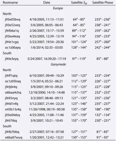
Table 2. List of the Detections of the Europa and Ganymede Footprint Tailsb Rootname Date SatelliteSIII Satellite Phase
Europa North j93e03bvq 4/18/2005, 11:13–11:51 64∘–85∘ 233∘–236∘ j93e52veq 5/6/2005, 06:05–06:43 64∘–85∘ 238∘–241∘ j9rlb6a1q 2/26/2007, 15:17–15:59 89∘–112∘ 259∘–262∘ j93ea4eaq 4/25/2005, 12:39–13:19 94∘–116∘ 230∘–233∘ j9rle1cgq 5/22/2007, 19:54–20:36 101∘–124∘ 257∘–260∘ oc1z06ayq 1/6/2014, 02:35–03:05 128∘–144∘ 242∘–244∘ South j9rle3eyq 5/24/2007, 16:39:20–17:19 97∘–119∘ 85∘–88∘ Ganymede North j9rlf1qtq 6/10/2007, 09:49–10:29 103∘–125∘ 233∘–234∘ oc1z05haq 1/5/2014, 05:52–06:21 112∘–129∘ 226∘–227∘ j9rlj6t4q 3/9/2007, 09:10–09:26 115∘–125∘ 227∘–228∘ o6baa4chq 12/18/2000, 14:10–14:48 115∘–137∘ 232∘–233∘ j9rli5nyq 3/2/2007, 08:48–09:13 121∘–135∘ 235∘–236∘ j9rld1nfq 5/12/2007, 21:44–22:24 123∘–146∘ 235∘–237∘ o43b13s4q 11/26/1998, 00:19–00:58 135∘–158∘ 188∘–190∘ j93e04dsq 4/25/2005, 11:08–11:46 137∘–159∘ 132∘–134∘ j9rli7tkq 3/9/2007, 10:21–10:45 155∘–170∘ 230∘–231∘ South j9rlb7bbq 2/27/2007, 07:16–07:58 127∘–151∘ 81∘–83∘ o6ba07wuq 1/20/2001, 12:42–13:21 130∘–153∘ 91∘–93∘
aThe number HST orbits for which the satellite’s phase angle lies between 90∘and 270∘is 62 for the northern EFP, 33 for the southern EFP, 70 for the northern GFP, and 44 for the southern GFP.
plasma sheet from south to north. This range also broadly corresponds the magnetic anomaly in the northern hemisphere. Moreover, Europa was in the dusk sector for all northern observations and in the dawn sector for the only southern observation. The observing geometry was thus also very similar, with the tail being close to the apparent ansa of the contour, a configuration favorable for limb brightening, which possibly facilitated the detection of this faint feature (see Figure 3 of Bonfond et al. [2013b] to better visualize this effect). It should, however, be noted that other image sets acquired in similar configurations did not lead to the identification of an EFP tail. Its brightness thus varies from one observation to another, similarly to the spots [Bonfond et al., 2017]. The brightness profile along the contour had a ∼ 5000 km plateau shape in the example studied by Grodent et al. [2006]. However, this profile may also display a more progressive decrease pattern with a e-folding length of ∼ 4000 km, which would correspond to approximately 14∘ of longitude when mapped into the equatorial plane (see Figure 2, top).
4.2.2. Ganymede Footprint Tail
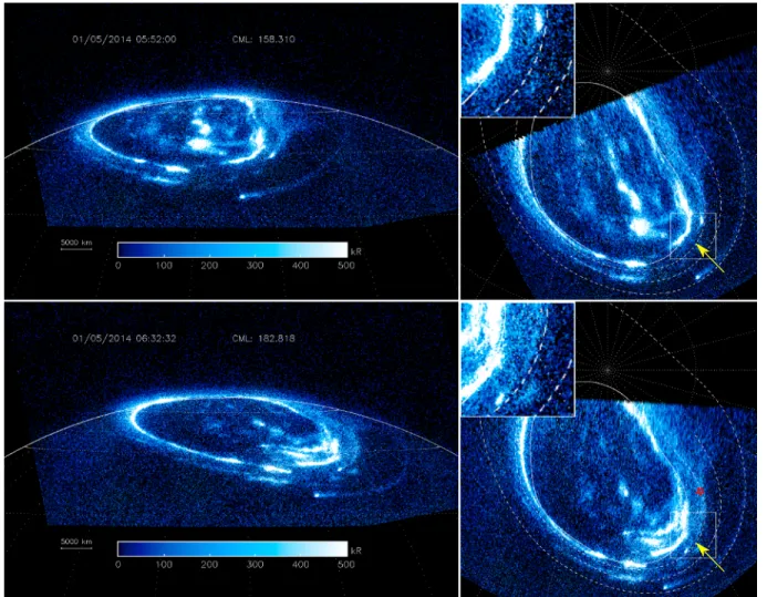
Figure 3 shows the polar projections of the first and last images acquired during a 45 min long HST obser-vation sequence acquired on 5 January 2014. It can clearly be seen on each image that the GFP MAW spot is followed by an arc of emission in the downstream direction. On individual images, it is not clear whether these emissions are actually related to Ganymede or if they are simply superposed to the GFP spot. However, the image sequence clearly demonstrates that at least a portion of these emissions are connected to the GFP because regions devoid of emissions in the first images (see the yellow arrow) only become bright after the passage of the GFP main spot. The SIIIlongitude of Ganymede changed from 112∘ to 136∘ during the
sequence. Ganymede was thus close to the center of the plasma sheet. Moreover, this indicates that the GFP tail was at least 24∘ long. While some of the emission on the dusk flank of the outer emissions most probably correspond to either the pitch angle diffusion boundary auroral signatures [Radioti et al., 2009] or auroral
Figure 2. Brightness profile along (top) the EFP and (bottom) the GFP. They originate from STIS time-tag imaging observations acquired on 6 and 5 January 2014 (see also Figure 3). No geometrical correction (i.e., limb brightening) is applied, and the uncertainty associated with the Poisson distribution of the counts is shown with dashed lines. In these two examples, the EFP tail profile drops rapidly while the GFP tail profile remains relatively constant over a long distance. The relative contribution of limb brightening and variations of the magnetic surface field to the apparent tail brightness are unclear.
injection signatures [Mauk et al., 2002; Dumont et al., 2014], it is nevertheless very likely that the tail seen on the last image continues beyond the location of the main spot on the first image. For example, the red star in Figure 3 maps to a point ∼30∘ downstream of Ganymede. Figure 2 (bottom) shows the brightness profile along the GFP contour for the last 500 s of this time-tag sequence. The brightness of this GFP tail decreases much more slowly than the one of the EFP.
A reinvestigation of the image database has lead to the identification of 9 other cases displaying a GFP tail in the northern hemisphere out of 70. Two additional cases have been identified in the southern hemisphere out of 44 (Table 2). Again, this detection rate is low relative to the number of HST orbits for which Ganymede’s phase angle lies between 90∘ and 270∘. Similarly to the Europa case, all of these cases are confined in a limited Ganymede longitude range (103∘ –170∘), even if this range is slightly shifted compared to the range found at Europa. In this range, Ganymede is leaving the plasma sheet center and approaching its northernmost centrifugal latitude.
4.2.3. Variability of the Io Footprint Tail Length
The IFP is located equatorward of any other auroral emission. The only exception, during which a blob of dif-fuse emissions was observed down to the latitude of the IFP, was documented by Bonfond et al. [2012]. In addition to being fixed in System III, the latitudinal extent of this feature was large and could not be mistaken for a much narrower (∼1000 km) footprint tail. As a consequence, the Io footprint tail can easily and system-atically be isolated and identified, contrary to the above mentioned EFP and GFP tails. Figure 4 (left) shows an exceptional case where an arc ∼20 kR above the background and colocated with the IFP reference contour emerges over the dawn limb>320∘ downstream of the MAW spot. Because this arc is located exactly where an IFP tail would be and because secondary auroral arcs have never been observed so far equatorward, its
attri-Figure 3. Images and polar projections of the northern aurora at the beginning and at the end of the sequence acquired on 5 January 2014. The solid line in the polar projection is the main emission reference oval from February 2007 [Bonfond et al., 2012]. The yellow arrows point toward the very same point in aSIIIfixed reference frame. This location was devoid of emission at the beginning of the sequence, and the emissions following the main GFP spot can thus be attributed to the GFP trail. The Io, Europa, and Ganymede footprint reference contours are shown with dashed lines in the polar projections. The main emission reference oval (February 2007) is shown in solid line. Tabulated values of these reference ovals are given in the supporting information.
bution to the IFP tail seems obvious. Interestingly, other image sets acquired in similar configurations (e.g., Figure 4 (right)) do not show any hint of such a long tail, indicating that its length, or at least, its brightness profile along the contour, may change with time.
5. Discussion and Conclusions
Early models of the Io footprint tail postulated a different mechanism to explain the spots and the tail: the spots would result from Alfvénic processes, while the tail would be generated by quasi-static processes [e.g., Delamere et al., 2003]. However, observations of the IFP above the limb showed that both the MAW spot and the tail have a similar vertical brightness profile [Bonfond et al., 2009; Bonfond, 2010]. This vertical pro-file is particularly broad (1200 km FWHM), and Monte Carlo simulations of the vertical propro-file indicated that only a broad energy distribution of the precipitating electrons, such as a kappa distribution, could fit the observations. The similarity of the vertical profile between the MAW spot and the tail suggests that the tail might also be Alfvénic in nature, as a result of an increasingly intricate reflection pattern for the Alfvén waves downstream of Io [Connerney and Satoh, 2000; Jacobsen et al., 2007, 2010]. We push this idea further here by showing that according to both model families, the tail length has the same dependence on the relevant phys-ical parameters, such as plasma density, plasma velocity, and magnetic field strength. To the first order, the footprint tail length is thus not a suitable parameter to differentiate the two kinds of models when we cross compare the auroral footprints of Io, Europa, and Ganymede. The length of the EFP and GFP tails derived from
Figure 4. Summed polar projections of the southern aurora on (left) 28 December 2000 and (right) 11 June 2007. The inner curve is the main emission reference oval from February 2007 [Bonfond et al., 2012] and the outer curve is the Io footprint reference oval [Bonfond et al., 2009]. The yellow arrow points toward a faint arc of emission collocated with the IFP contour and thus attributed to the IFP tail. In the other case, the observing geometry was similar but no hint of a tail can be seen above the dawn limb. The Io footprint reference contour and the main emission reference oval (February 2007) are shown in solid line. Tabulated values of these reference ovals are given in the supporting information.
our observations, ∼14∘ and⩾24∘ for Europa and Ganymede, respectively, lies within a factor of 2–3 relative to estimates from the theoretical model of Hill and Vasyli¯unas [2002] (𝜑Europa0 ≈ 6∘ and𝜑Ganymede0 ≈ 11∘), which may be considered as a fair agreement, acknowledging the variability of the plasma parameters at the satellite. On the other hand, Matsuda et al. [2012] challenged the idea that the vertical emission profile could actually be a reliable parameter to decide between them. They suggested that the evolution of the pitch angle distri-bution from quasi-parallel to the magnetic field at the acceleration site to horseshoe in the upper atmosphere, together with the mirroring of backscattered electrons could both broaden the vertical emission profile, even in the case of quasi-static electric fields. However, our new Monte Carlo simulations taking these two effects into account show that they only marginally modify the vertical emission profile and cannot account for the observed profile.
A reanalysis of the database of far UV images of the Jovian aurorae leads to the finding of footprint tails for both the EFP and the GFP and in both the hemisphere. This is an important result, because the nature of the local interaction is different at the three satellites: Io’s being dominated by its neutral sources, Europa’s by its induced magnetic field, and Ganymede’s by its intrinsic magnetic field [Jia et al., 2009b]. This further indicates that all footprints are the same [cf. Bonfond et al., 2017], in the sense that they all share the same morphology and thus most probably arise from the same mechanisms, despite the initial local differences. The finding of a GFP tail demonstrates that intense mass loading is not required to produce a footprint tail.
Even if the IFP shows some variability from one observation to another [Bonfond et al., 2013b], the temporal brightness and morphological variabilities are greater for the EFP and the GFP, both for the spots and the tails. Indeed, the tails of the EFP and GFP are only seldom seen, even in similar configurations. It is, however, likely that a more sensitive instrument would detect faint tail where we see none with HST’s current cameras. Nevertheless, the clustering of the detection events in the same longitude range is not likely solely due to a combination of selection bias and peculiar observing geometry favoring limb brightening on the dusk or dawn flanks. If the Alfvénic model for the tails is correct, as our new simulation suggests for the IFP tail, then it is expected that Alfvén waves’ reflections preferentially occur when the satellite lies within the plasma sheet and then persist for some time as the waves are partially trapped between density gradients and bounce back and forth for several tens of minutes. Since Io is always located within the torus, the tail would always be present, in accordance with the observations. Varying plasma conditions (density, temperature, composition, etc.) may trap the waves for a varying amount of time, sometimes leading to a longer tail than usual, as for the unusually long IFP tail showed in Figure 4.
References
Bisikalo, D. V., and V. I. Shematovich (2015), Precipitation of electrons into the upper atmosphere of a hot-Jupiter exoplanet, Astron. Rep., 59, 836–842, doi:10.1134/S1063772915090024.
Bonfond, B. (2010), The 3-D extent of the Io UV footprint on Jupiter, J. Geophys. Res., 115, A09217, doi:10.1029/2010JA015475.
Bonfond, B., D. Grodent, J.-C. Gérard, A. Radioti, J. Saur, and S. Jacobsen (2008), UV Io footprint leading spot: A key feature for understanding the UV Io footprint multiplicity?, Geophys. Res. Lett., 35, L05107, doi:10.1029/2007GL032418.
Bonfond, B., D. Grodent, J.-C. Gérard, A. Radioti, V. Dols, P. A. Delamere, and J. T. Clarke (2009), The Io UV footprint: Location, inter-spot distances and tail vertical extent, J. Geophys. Res., 114, A07224, doi:10.1029/2009JA014312.
Bonfond, B., M. F. Vogt, J.-C. Gérard, D. Grodent, A. Radioti, and V. Coumans (2011), Quasi-periodic polar flares at Jupiter: A signature of pulsed dayside reconnections?, Geophys. Res. Lett., 380, L02104, doi:10.1029/2010GL045981.
Bonfond, B., D. Grodent, J.-C. Gérard, T. Stallard, J. T. Clarke, M. Yoneda, A. Radioti, and J. Gustin (2012), Auroral evidence of Io’s control over the magnetosphere of Jupiter, Geophys. Res. Lett., 39, L01105, doi:10.1029/2011GL050253.
Bonfond, B., S. Hess, F. Bagenal, J.-C. Gérard, D. Grodent, A. Radioti, J. Gustin, and J. T. Clarke (2013a), The multiple spots of the Ganymede auroral footprint, Geophys. Res. Lett., 40, 4977–4981, doi:10.1002/grl.50989.
Bonfond, B., S. Hess, J.-C. Gérard, D. Grodent, A. Radioti, V. Chantry, J. Saur, S. Jacobsen, and J. T. Clarke (2013b), Evolution of the Io footprint brightness I: Far-UV observations, Planet. Space Sci., 88, 64–75, doi:10.1016/j.pss.2013.05.023.
Bonfond, B., S. Grodent, S. V. Badman, J. Saur, J.-C. Gérard, and A. Radioti (2017), Similarity of the Jovian satellite footprints: spots multiplicity and dynamics, Icarus, 292, 208–217, doi:10.1016/j.icarus.2017.01.009.
Clarke, J. T., et al. (2002), Ultraviolet emissions from the magnetic footprints of Io, Ganymede and Europa on Jupiter, Nature, 415, 997–1000. Connerney, J. E. P., and T. Satoh (2000), The H+3ion: A remote diagnostic of the Jovian magnetosphere, in Astronomy, Physics and Chemistry
of H+3, p. 2471, Royal Society, England.
Connerney, J. E. P., R. Baron, T. Satoh, and T. Owen (1993), Images of excitedH+
3at the foot of the Io flux tube in Jupiter’s atmosphere, Science, 262, 1035–1038.
Delamere, P. A., F. Bagenal, R. Ergun, and Y.-J. Su (2003), Momentum transfer between the Io plasma wake and Jupiter’s ionosphere, J. Geophys. Res., 108, 11–1, doi:10.1029/2002JA009530.
Dols, V., P. A. Delamere, and F. Bagenal (2008), A multispecies chemistry model of Io’s local interaction with the Plasma Torus, J. Geophys. Res., 113, A09208, doi:10.1029/2007JA012805.
Duling, S., J. Saur, and J. Wicht (2014), Consistent boundary conditions at nonconducting surfaces of planetary bodies: Applications in a new Ganymede MHD model, J. Geophys. Res. Space Physics, 119, 4412–4440, doi:10.1002/2013JA019554.
Dumont, M., D. Grodent, A. Radioti, B. Bonfond, and J.-C. Gérard (2014), Jupiter’s equatorward auroral features: Possible signatures of magnetospheric injections, J. Geophys. Res. Space Physics, 119, 10,068–10,077, doi:10.1002/2014JA020527.
Ergun, R. E., Y.-J. Su, L. Andersson, F. Bagenal, P. A. Delemere, R. L. Lysak, and R. J. Strangeway (2006), S bursts and the Jupiter ionospheric Alfvén resonator, J. Geophys. Res., 111, A06212, doi:10.1029/2005JA011253.
Eviatar, A., and C. Paranicas (2005), The plasma plumes of Europa and Callisto, Icarus, 178, 360–366, doi:10.1016/j.icarus.2005.06.007. Frank, L. A., and W. R. Paterson (1999), Intense electron beams observed at Io with the Galileo spacecraft, J. Geophys. Res., 104,
28,657–28,669.
Frank, L. A., and W. R. Paterson (2002), Plasmas observed with the Galileo spacecraft during its flyby over Io’s northern polar region, J. Geophys. Res., 107, 1220, doi:10.1029/2002JA009240.
Gérard, J.-C., B. Hubert, D. V. Bisikalo, and V. I. Shematovich (2000), A model of the Lyman-𝛼line profile in the proton aurora, J. Geophys. Res., 105, 15,795–15,806, doi:10.1029/1999JA002002.
Gérard, J.-C., A. Saglam, D. Grodent, and J. T. Clarke (2006), Morphology of the ultraviolet Io footprint emission and its control by Io’s location, J. Geophys. Res., 111, A04202, doi:10.1029/2005JA011327.
Gérard, J.-C., B. Bonfond, J. Gustin, D. Grodent, J. T. Clarke, D. Bisikalo, and V. Shematovich (2009), Altitude of Saturn’s aurora and its implications for the characteristic energy of precipitated electrons, Geophys. Res. Lett., 36, L02202, doi:10.1029/2008GL036554. Goertz, C. K. (1980), Io’s interaction with the plasma torus, J. Geophys. Res., 85, 2949–2956, doi:10.1029/JA085iA06p02949. Grodent, D. (2015), A brief review of ultraviolet auroral emissions on giant planets, Space Sci. Rev., 187, 23–50,
doi:10.1007/s11214-014-0052-8.
Grodent, D., J. Waite, and J.-C. Gérard (2001), A self-consistent model of the Jovian auroral thermal structure, J. Geophys. Res., 106, 12,933–12,952, doi:10.1029/2000JA900129.
Grodent, D., J.-C. Gérard, J. Gustin, B. H. Mauk, J. E. P. Connerney, and J. T. Clarke (2006), Europa’s FUV auroral tail on Jupiter, Geophys. Res. Lett., 33, L06201, doi:10.1029/2005GL025487.
Grodent, D., B. Bonfond, J.-C. Gérard, A. Radioti, J. Gustin, J. T. Clarke, J. Nichols, and J. E. P. Connerney (2008), Auroral evidence of a localized magnetic anomaly in Jupiter’s northern hemisphere, J. Geophys. Res., 113, A09201, doi:10.1029/2008JA013185.
Gustin, J., B. Bonfond, D. Grodent, and J. C. Gérard (2012), Conversion from HST ACS and STIS auroral counts into brightness, precipitated power and radiated power for H2giant planets J., J. Geophys. Res., 117, A07316, doi:10.1029/2012JA017607.
Hess, S., B. Bonfond, V. Chantry, J.-C. Gérard, D. Grodent, S. Jacobsen, and A. Radioti (2013), Evolution of the Io footprint brightness II: Modeling, Planet. Space Sci., 88, 76–85.
Hess, S. L. G., P. Delamere, V. Dols, B. Bonfond, and D. Swift (2010), Power transmission and particle acceleration along the Io flux tube, J. Geophys. Res., 115, A06205, doi:10.1029/2009JA014928.
Hill, T. W., and V. M. Vasyli ¯unas (2002), Jovian auroral signature of Io’s corotational wake, J. Geophys. Res., 107, 27–1, doi:10.1029/2002JA009514.
Hinson, D. P., A. J. Kliore, F. M. Flasar, J. D. Twicken, P. J. Schinder, and R. G. Herrera (1998), Galileo radio occultation measurements of Io’s ionosphere and plasma wake, J. Geophys. Res., 103, 29,343–29,358, doi:10.1029/98JA02659.
Jacobsen, S., F. M. Neubauer, J. Saur, and N. Schilling (2007), Io’s nonlinear MHD-wave field in the heterogeneous Jovian magnetosphere, Geophys. Res. Lett., 34, L10202, doi:10.1029/2006GL029187.
Jacobsen, S., J. Saur, F. M. Neubauer, B. Bonfond, J.-C. Gérard, and D. Grodent (2010), Location and spatial shape of electron beams in Io’s wake, J. Geophys. Res., 115, A04205, doi:10.1029/2009JA014753.
Jia, X., R. J. Walker, M. G. Kivelson, K. K. Khurana, and J. A. Linker (2009a), Properties of Ganymede’s magnetosphere inferred from improved three-dimensional MHD simulations, J. Geophys. Res., 114, A09209, doi:10.1029/2009JA014375.
Jia, X., M. G. Kivelson, K. K. Khurana, and R. J. Walker (2009b), Magnetic fields of the satellites of Jupiter and Saturn, Space Sci. Rev., 152, 271–305, doi:10.1007/s11214-009-9507-8.
Acknowledgments
B.B. would like to thank Zhonghua Yao for helpful discussions. B.B., D.G., A. R., and J.-C.G. were supported by the PRODEX program managed by ESA in collaboration with the Belgian Federal Science Policy Office. S.V.B. was supported by an STFC Ernest Rutherford Fellowship. D.B. and V.S. were supported by the Russian Science Foundation. This research is based on publicly available observations acquired with the NASA/ESA Hubble Space Telescope and obtained at the Space Telescope Science Institute, which is operated by AURA for NASA (program IDs 7308, 7769, 8171, 8657, 10140, 10507, 10862, 12883, and 13035) (https://archive.stsci.edu/ hst/search.php).
Jones, S. T., and Y.-J. Su (2008), Role of dispersive Alfvén waves in generating parallel electric fields along the Io-Jupiter fluxtube, J. Geophys. Res., 113, A12205, doi:10.1029/2008JA013512.
Kivelson, M. G., K. K. Khurana, D. J. Stevenson, L. Bennett, S. Joy, C. T. Russell, R. J. Walker, C. Zimmer, and C. Polanskey (1999), Europa and Callisto: Induced or intrinsic fields in a periodically varying plasma environment, J. Geophys. Res., 104, 4609–4626, doi:10.1029/1998JA900095.
Kivelson, M. G., F. Bagenal, W. S. Kurth, F. M. Neubauer, C. Paranicas, and J. Saur (2004), Magnetospheric interactions with satellites, in Jupiter, pp. 513–536, The Planet, Satellites and Magnetosphere, Cambridge Univ. Press, Cambridge, U. K.
Matsuda, K., N. Terada, Y. Katoh, and H. Misawa (2012), A simulation study of the current-voltage relationship of the Io tail aurora, J. Geophys. Res., 117, A10214, doi:10.1029/2012JA017790.
Mauk, B. H., J. T. Clarke, D. Grodent, J. H. Waite, C. P. Paranicas, and D. J. Williams (2002), Transient aurora on Jupiter from injections of magnetospheric electrons, Nature, 415, 1003–1005.
Motoba, T., and M. Hirahara (2016), High-resolution auroral acceleration signatures within a highly dynamic onset arc, Geophys. Res. Lett., 43, 1793–1801, doi:10.1002/2015GL067580.
Neubauer, F. M. (1980), Nonlinear standing Alfven wave current system at Io—Theory, J. Geophys. Res., 85, 1171–1178.
Neubauer, F. M. (1998), The sub-Alfvénic interaction of the Galilean satellites with the Jovian magnetosphere, J. Geophys. Res., 103, 19,843–19,866, doi:10.1029/97JE03370.
Paschmann, G., S. Haaland, and R. Treumann (2002), Chapter 4—In situ measurements in the auroral plasma, Space Sci. Rev., 103(1), 93–208, doi:10.1023/A:1023082700768.
Paty, C., W. Paterson, and R. Winglee (2008), Ion energization in Ganymede’s magnetosphere: Using multifluid simulations to interpret ion energy spectrograms, J. Geophys. Res., 113, A06211, doi:10.1029/2007JA012848.
Pryor, W. R., et al. (2011), The auroral footprint of Enceladus on Saturn, Nature, 472, 331–333, doi:10.1038/nature09928.
Radioti, A., A. T. Tomás, D. Grodent, J.-C. Gérard, J. Gustin, B. Bonfond, N. Krupp, J. Woch, and J. D. Menietti (2009), Equatorward diffuse auroral emissions at Jupiter: Simultaneous HST and Galileo observations, Geophys. Res. Lett., 36, L07101, doi:10.1029/2009GL037857. Saur, J. (2004), A model of Io’s local electric field for a combined Alfvénic and unipolar inductor far-field coupling, J. Geophys. Res., 109,
A01210, doi:10.1029/2002JA009354.
Saur, J., F. M. Neubauer, D. F. Strobel, and M. E. Summers (1999), Three-dimensional plasma simulation of Io’s interaction with the Io plasma torus: Asymmetric plasma flow, J. Geophys. Res., 104, 25,105–25,126, doi:10.1029/1999JA900304.
Saur, J., T. Grambusch, S. Duling, F. M. Neubauer, and S. Simon (2013), Magnetic energy fluxes in sub-Alfvénic planet star and moon planet interactions, Astron. Astrophys., 552, A119, doi:10.1051/0004-6361/201118179.
Shematovich, V. I., D. V. Bisikalo, J.-C. Gérard, C. Cox, S. W. Bougher, and F. Leblanc (2008), Monte Carlo model of electron transport for the calculation of Mars dayglow emissions, J. Geophys. Res., 113, E02011, doi:10.1029/2007JE002938.
Strobel, D. F., and S. K. Atreya (1983), Physics of the Jovian magnetosphere, in Ionosphere, chap 2., pp. 51–67, Cambridge Univ. Press, New York.
Su, Y.-J., R. E. Ergun, F. Bagenal, and P. A. Delamere (2003), Io-related Jovian auroral arcs: Modeling parallel electric fields, J. Geophys. Res., 108, 1094, doi:10.1029/2002JA009247.
Weiss, J. W. (2004), Jupiter: The planet, satellites and magnetosphere, in Planetary Parameters, chap. Appendix 2., pp. 699–706, Cambridge Univ. Press, Cambridge, U. K.
![Table 1. List of the Relevant Parameters to Compute the Length of the Footprint Tails According to the Model of Hill and Vasyli¯unas [2002] a](https://thumb-eu.123doks.com/thumbv2/123doknet/5944648.146617/2.918.348.782.179.288/table-relevant-parameters-compute-length-footprint-according-vasyli.webp)