HAL Id: hal-02624896
https://hal.inrae.fr/hal-02624896
Submitted on 23 Nov 2020HAL is a multi-disciplinary open access archive for the deposit and dissemination of sci-entific research documents, whether they are pub-lished or not. The documents may come from teaching and research institutions in France or abroad, or from public or private research centers.
L’archive ouverte pluridisciplinaire HAL, est destinée au dépôt et à la diffusion de documents scientifiques de niveau recherche, publiés ou non, émanant des établissements d’enseignement et de recherche français ou étrangers, des laboratoires publics ou privés.
Distributed under a Creative Commons Attribution - NonCommercial - NoDerivatives| 4.0 International License
differentiation in Arvicola water voles (Rodentia,
Cricetidae)
Pascale Chevret, Sabrina Renaud, Zeycan Helvaci, Rainer Ulrich, Jean-pierre
Quéré, Johan Michaux
To cite this version:
Pascale Chevret, Sabrina Renaud, Zeycan Helvaci, Rainer Ulrich, Jean-pierre Quéré, et al.. Ge-netic structure, ecological versatility, and skull shape differentiation in Arvicola water voles (Roden-tia, Cricetidae). Journal of Zoological Systematics and Evolutionary Research, Wiley, 2020, 58 (4), pp.1323-1334. �10.1111/jzs.12384�. �hal-02624896�
3
Short running title: Arvicola phylogeography and morphometry
4 5
Pascale Chevret 1, Sabrina Renaud 1, Zeycan Helvaci 2,3, Rainer Ulrich 4, Jean-Pierre Quéré 5, 6
Johan R. Michaux 2, 6 7
8
1 Laboratoire de Biométrie et Biologie Evolutive, UMR 5558, CNRS, Université Claude 9
Bernard Lyon 1, Université de Lyon, Villeurbanne, France 10
2 Conservation Genetics Laboratory, Institut de Botanique, Chemin de la Vallée, 4, 4000 11
Liège, Belgium 12
3 Present address: Aksaray Üniversitesi Fen Edebiyat Fakültesi, 68100 Merkez/ Aksaray, 13
Turkey 14
4 Institute of Novel and Emerging Infectious Diseases,Friedrich-Loeffler-Institut, Federal 15
Research Institute for Animal Health, Südufer 10, 17493 Greifswald - Insel Riems, Germany 16
5 Centre de Biologie et Gestion des Populations (INRA / IRD / Cirad /Montpellier SupAgro), 17
Campus international de Baillarguet, CS 30016, F-34988, Montferrier-sur-Lez Cedex, France 18
6 CIRAD/INRA UMR117 ASTRE, Campus International de Baillarguet, 34398 Montpellier 19
Cedex 5, France 20
21
Corresponding author: Pascale Chevret, e-mail: pascale.chevret@univ-lyon1.fr 22
23
Keywords: Phylogeography, geometric morphometrics, cytochrome b, Arvicola amphibius,
24
plasticity 25
26 27
28
Abstract
29 30
Water voles from the genus Arvicola display an amazing ecological versality, with aquatic 31
and fossorial populations. The Southern water vole (A. sapidus) is largely accepted as a valid 32
species, as well as the newly described A. persicus. In contrast, the taxonomic status and 33
evolutionary relationships within A. amphibius sensu lato had caused a long-standing debate. 34
The phylogenetic relationships among Arvicola were reconstructed using the mitochondrial 35
cytochrome b gene. Four lineages within A. amphibius s. l. were identified with good support: 36
Western European, Eurasiatic, Italian, and Turkish lineages. Fossorial and aquatic forms were 37
found together in all well-sampled lineages, evidencing that ecotypes do not correspond to 38
distinct species. However, the Western European lineage mostly includes fossorial forms 39
whereas the Eurasiatic lineage tend to include mostly aquatic forms. A morphometric analysis 40
of skull shape evidenced a convergence of aquatic forms of the Eurasiatic lineage towards the 41
typically aquatic shape of A. sapidus. The fossorial form of the Western European lineage, in 42
contrast, displayed morphological adaptation to tooth-digging behavior, with expanded 43
zygomatic arches and proodont incisors. Fossorial Eurasiatic forms displayed intermediate 44
morphologies. This suggest a plastic component of skull shape variation, combined with a 45
genetic component selected by the dominant ecology in each lineage. Integrating genetic 46
distances and other biological data suggest that the Italian lineage may correspond to an 47
incipient species (A. italicus). The three other lineages most probably correspond to 48
phylogeographic variations of a single species (A. amphibius), encompassing the former A. 49
amphibius, A. terrestris, A. scherman and A. monticola.
50 51 52
Introduction
53 54
The extension of phylogeographical studies has led to the increasing recognition that many 55
species traditionally identified based on morphological traits encompass several genetic 56
distinct forms that constitute “cryptic species” [e.g. (Bryja et al., 2014; Mouton et al., 2017)]. 57
Slow morphological divergence, as a probable consequence of stabilizing selection, may be 58
responsible for the limited phenotypic signature of these cryptic species. Yet, morphology, 59
inclusive osteological traits, varies according to ecological conditions, including diet 60
(Michaux, Chevret, & Renaud, 2007) but also way-of-life such as digging behavior, which 61
exerts strong functional demands on the skull (Gomes Rodrigues, Šumbera, & Hautier, 2016). 62
As a consequence, ecological versatility may lead to morphological convergence blurring the 63
signature of genetic divergence between species. Assessing the evolutionary units involved in 64
such cases is crucial to understand the selective context driving the genetic and morphological 65
divergence. 66
Water voles of the genus Arvicola constitute an emblematic example of the controversies that 67
may arise regarding ecological forms. Fossorial and semi-aquatic forms have been described 68
as species (A. terrestris, Linnaeus, 1758, type locality Uppsala, Sweden and A. amphibius, 69
Linnaeus, 1758, type locality England) already by Linnaeus in 1758. Later on, up to seven 70
species have been described (Miller et al., 2012). By combining chromosomal and ecological 71
data, only three species were thereafter proposed (Heim de Balsac & Guislain, 1955): the 72
Southern water vole A. sapidus, Miller, 1908, with 2n = 40, A. terrestris for semi-aquatic 73
forms with 2n = 36, and A. scherman, Shaw, 1801, for fossorial forms with 2n = 36. 74
The status of A. sapidus was subject to little debate but controversy persisted regarding the 75
aquatic and fossorial forms A. terrestris/A. scherman: considered as a single polytypic species 76
(Wilson & Reeder, 1993), or valid distinct species: A. amphibius and A. scherman (Wilson & 77
Reeder, 2005). More recently, the Italian water vole was proposed as a separate species (A. 78
italicus, Savi, 1839) (Castiglia et al., 2016), while the aquatic and fossorial forms remained
79
considered as separate species with distinct geographic distribution, under the names of A. 80
amphibius and A. monticola, de Sélys Longchamps, 1838 (Pardiñas et al., 2017). Even more
81
recently, Mahmoudi, Maul, Khoshyar, & Darvish (2019) identified in Iran another species, A. 82
persicus. Hence, the genus Arvicola currently includes five species: amphibius, italicus,
83
monticola, sapidus and persicus (Mahmoudi et al., 2019; Pardiñas et al., 2017).
84
Yet, an increasing genetic sampling brought new fuel in the debate, showing that the 85
ecological forms were not systematically associated with distinct clades. Fossorial and aquatic 86
forms have been found to coexist in the Italian water vole (Castiglia et al., 2016) and in A. 87
scherman (Kryštufek et al., 2015). The limited sampling of A. monticola precluded to reliably
88
asses the variation in this presumed fossorial clade (Mahmoudi et al., 2019). 89
The present study therefore aims at a clarification of the phylogenetic pattern within European 90
water voles, by compiling published and new cytochrome b sequences, with the aim to 91
improve the geographic coverage and representation of the two ecological forms. This genetic 92
approach was complemented by a morphometric analysis of skull shape variations of aquatic 93
and fossorial forms, in order to assess the patterns of morphological differentiation and 94
possible convergences. 95
96
Material and Methods
97 98
The terminology used thereafter is the following. The Southern water vole, A. sapidus, and 99
the Iranian water vole, A. persicus, were named by their Latin name. The other water voles 100
were designed as “water voles” or Arvicola amphibius considered sensu lato, hence including 101
both fossorial and aquatic water voles (including specimens labelled as amphibius, monticola, 102
scherman and terrestris). The status of the Italian water vole will be discussed, but the name
103
“italicus” was tentatively retained. 104
105
Material for genetics
106
The genetic sampling original to this study included 143 tissue samples of Arvicola amphibius 107
s. l. from Belgium, Denmark, France, Germany, Great Britain and Spain, two specimens
108
identified as A. scherman from Spain, as well as two samples of Arvicola sapidus (Table S1). 109
Most of the samples were attributed to fossorial or aquatic forms, based on field evidences: 110
fossorial forms were trapped in tumuli. It was completed with sequences available in 111
GenBank for A. amphibius (89), A. scherman (2), A. sapidus (12) and A. persicus (14) (Table 112
S1). The complete dataset for A. amphibius s. l. comprised 236 sequences from 102 localities 113
(Table S1, Figure 1A). 114
115
Material for morphometrics
116
The material available for morphometric studies (Table S2) corresponded to 223 skulls. It 117
included various fossorial populations from France and Western Switzerland. The Eurasiatic 118
lineage (sensu (Castiglia et al., 2016)) was sampled by aquatic populations from Finland, 119
Denmark, and Belgium. Water voles from Ticino in Southern Switzerland were labelled as 120
italicus and represented the Italian lineage (Brace et al., 2016; Castiglia et al., 2016).
121
Specimens from various localities in France and Spain represented the sister species A. 122
sapidus.
123
In three populations (Chapelle d’Huin, La Grave, and Prangins), sex information was 124
available and allowed to test for sexual dimorphism. Almost all specimens corresponded to 125
adult and sub-adult specimens. The specimens are stored in the collections of the Centre de 126
Biologie et Gestion des Populations (Baillarguet, Montferrier-sur-Lez, France), the Muséum 127
d’Histoire Naturelle (Geneva, Switzerland) and the Université de Liège (Belgium). 128
129
Genetic analysis
130
DNA was extracted from ethanol-preserved tissue of Arvicola, using the DNeasy Blood and 131
Tissue kit (Qiagen, France) following the manufacturer instructions. The cytochrome b gene 132
sequence was amplified using previously described primers L7 (5-133
ACCAATGACATGAAAAATCATCGTT-3) and H6 (5'-134
TCTCCATTTCTGGTTTACAAGAC-3') (Montgelard, Bentz, Tirard, Verneau, & Catzeflis, 135
2002). PCRs were carried out in 50 l volume containing 12.5 l of each 2 mM primers, 1 l 136
of 10 mM dNTP, 10 l of reaction buffer (Promega), 0.2 l of 5 U/l Promega Taq DNA 137
polymerase and approximately 30 ng of DNA extract. Amplifications were performed using 138
one activation step (94°C/4 min) followed by 40 cycles (94°C/30 s, 50°C/60 s, 72°C/90 s) 139
with a final extension step at 72°C for 10 min. PCR products (1243 bp long) were send to 140
Macrogen (Seoul, Korea) for sequencing. 141
The sequences generated were visualized and analyzed using Seqscape (Applied Biosystems) 142
or CLC Workbench (Qiagen) and aligned with Seaview v4 (Gouy, Guindon, Gascuel, & 143
Lyon, 2010). All the new sequences were submitted to GenBank: accession number 144
LR746349 to LR746495. The final alignment comprised 264 sequences of Arvicola, 147 new 145
ones and 117 retrieved from GenBank. Sequences of Microtus arvalis, Myodes glareolus, 146
Eothenomys melanogaster, and Ellobius tancrei were used as outgroups. This resulted in a
147
final alignment comprising 268 sequences and 911 positions (Alignment S1) after the removal 148
of the sites with more than 10% of missing data. The best model fitting our data (GTR+I+G) 149
was selected with jModelTest (Darriba, Taboada, Doallo, & Posada, 2012) using the Akaike 150
criterion (Akaike, 1973). The phylogenetic tree was reconstructed using maximum likelihood 151
with PhyMl 3.0 (Guindon et al., 2010) and Bayesian inference with MrBayes v3.2 (Ronquist 152
et al., 2012). Robustness of the nodes were estimated with 1000 boostrap replicates with 153
PhyMl and posterior probability with MrBayes. Markov chain Monte Carlo (MCMC) 154
analyses were run independently for 20 000 000 generations with one tree sampled every 500 155
generations. The burn-in was graphically determined with Tracer v1.6 (A. Rambaut, Suchard, 156
Xie, & Drummond, 2014). We also checked that the effective sample sizes (ESSs) were 157
above 200 and that the average standard deviation of split frequencies remained <0.05 after 158
the burn-in threshold. We discarded 10% of the trees and visualized the resulting tree with 159
Figtree v1.4 (Rambaut, 2012). MEGA 7 (Kumar, Stecher, & Tamura, 2016) was used to 160
estimate K2P distance between and within lineages. We use POPART (Leigh & Bryant, 161
2015) to reconstruct a median joining network of haplotypes (Bandelt, Forster, & Rohl, 162
1999). This analysis was restricted to the 236 sequences of A. amphibius, and the 163
corresponding haplotypes were determined with DnaSP v6 (Rozas et al., 2017). 164
165
Morphometric analyses
166
Each skull was photographed in ventral and lateral views using a Canon EOS 400D digital 167
camera. The ventral view was described by a configuration of 22 landmarks and 13 sliding 168
semi-landmarks along the zygomatic arch. The lateral view was described using a 169
configuration of 24 landmarks and 39 sliding semi-landmarks (Figure S1). All landmarks and 170
sliding semi-landmarks were digitized using TPSdig2 (Rohlf, 2010). The sampling included 171
189 skulls in ventral view and 186 ones in lateral view (Table S2). 172
The configurations of landmarks and semi-landmarks were superimposed using a generalized 173
Procrustes analysis (GPA) standardizing size, position and orientation while retaining the 174
geometric relationships between specimens (Rohlf & Slice, 1990). During the 175
superimposition, semi-landmarks were allowed sliding along their tangent vectors until their 176
positions minimize the shape between specimens, the criterion being here bending energy 177
(Bookstein, 1997). A Principal Component Analysis (PCA) was performed on the resulting 178
aligned coordinates. Relationships between difference groups were investigated using a 179
Canonical Variate Analysis (CVA) which aims at separating groups by looking for linear 180
combinations of variables that maximize the between-group to within-group variance ratio. 181
By standardizing within-group variance, this method may be efficient for evidencing 182
phylogenetic relationships (Renaud, Dufour, Hardouin, Ledevin, & Auffray, 2015). In order 183
to reduce the dimensionality of the data, the CVA was performed on the set of Principal 184
Components (PC) totaling more than 95% of the variance. 185
Skull size was estimated using the centroid size (square root of the sum of the squared 186
distances from each landmark to the centroid of the configuration). Size differences were 187
tested using analyses of variance (ANOVA). 188
Geometric differences between groups and regression models were investigated using 189
procedures adapted for Procrustes data (Procrustes ANOVA). Using this approach, the 190
Procrustes distances among specimens are used to quantify explained and unexplained 191
components of shape variation, which are statistically evaluated via permutation (here, 9999 192
permutations) (Adams et Otárola-Castillo 2013). Allometric variations were investigated, 193
investigating skull shape as a function of skull size. The effect of a grouping variable 194
combining genetic and ecological information (“GxE”) was also included (Table S2), 195
allowing to test if the allometric slopes were different between the groups. Visualization were 196
obtained using the Common Allometric Component (CAC) derived from this allometry 197
analysis (Adams et al. 2013). Procrustes superimposition, PCA and Procrustes ANOVA were 198
performed using the R package geomorph (Adams & Otárola-Castillo, 2013). The CVA was 199
computed using the package Morpho (Schlager, 2017). 200 201 Results 202 203 Genetics 204
On the phylogenetic tree (Figure 2, see Figure S2 for the complete phylogeny) the three 205
groups corresponding to A. sapidus, persicus and amphibius s. l. were well supported 206
(PP≥0.93, BP≥82) with A. amphibius more closely related to A. persicus (PP=0,93, PP=72) 207
than to A. sapidus. The phylogenetic tree as well as the network (Figure 1B) evidenced four 208
lineages within A. amphibius s. l.. Most of the sequences of amphibius s. l. belonged to two 209
lineages: Lineage 1 (L1) and Lineage 2 (L2). L1 was present in France, Spain, Switzerland 210
and the North of Great Britain and comprises mostly fossorial forms. This lineage was 211
divided into two sub-groups: the first one with samples from France and Spain and the second 212
one with samples from Great Britain, Switzerland and France. The two specimens identified 213
as A. scherman belonged to this lineage. L2 had a large repartition area from the south of 214
Great Britain to Russia (East), Finland (North) and Romania (South) and it comprised more 215
aquatic than fossorial forms. The two remaining lineages were restricted to Turkey, Lineage 3 216
(L3) with aquatic forms only and Italy, Lineage 4 (L4) with both aquatic and fossorial forms 217
(Figure 2, Figure S2 and Figure 1C). In several French localities (Chapelle d’Huin, Doubs; 218
Val d’Ajol, Vosges; Vauconcourt, Haute-Saône; Vigeois, Corrèze), a co-occurrence of 219
lineages 1 and 2 was documented. In all cases, L1 was dominant and the population mostly 220
fossorial. 221
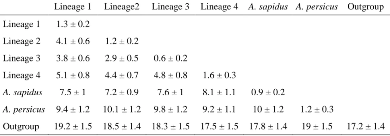
Regarding the amount of genetic divergence, A. sapidus, A. persicus and A. amphibius s. l. 222
appeared well differentiated (K2P distances ≥ 7.2). L3 was closely related to L2 (K2P = 2.9) 223
whereas L4, which correspond to A. italicus, was the most divergent (4.4 < K2P < 5.1) within 224 A. amphibius s. l. (Table 1). 225 226 Morphometrics 227
Sexual dimorphism. – Sexes displayed very similar skull size and shape. No difference was 228
detected for the size of the skull in ventral view (ANOVA on Ventral Centroid Size: Chapelle 229
d’Huin P = 0.3031; La Grave P = 0.8706; Prangins P = 0.9799) and in lateral view (ANOVA 230
on Lateral Centroid Size: Chapelle d’Huin P = 0.1358; La Grave P = 0.3575; Prangins P = 231
0.9576). Similarly, skull shape was not different between sexes, for the skull in ventral view 232
(Procrustes ANOVA on ventral skull shape: Chapelle d’Huin P = 0.6130; La Grave P = 233
0.4556; Prangins P = 0.8309) as for the skull in lateral view (Procrustes ANOVA on lateral 234
skull shape: Chapelle d’Huin P = 0.1918; La Grave P = 0.4337; Prangins P = 0.7164). All 235
animals were therefore pooled in subsequent analyses. 236
Skull size. – The different groups of water voles significantly differed in skull size (ANOVA 237
on CSventral and CSlateral: P < 0.0001). Skulls of water voles, being fossorial or aquatic, 238
were smaller than those of A. sapidus (Figure 3). Important size variation occurred within A. 239
amphibius s.l.. The aquatic populations of L2 were especially variable in size, the Belgian one
240
being almost as large as A. sapidus whereas skulls from Finnish A. amphibius were among the 241
smallest. Important size variation also occurred within populations belonging to L1. 242
Skull shape in ventral view. – The variation of skull shape in ventral view was structured in 243
two groups on the first two axes of a PCA on the aligned coordinates (Figure 4A). These two 244
groups opposed aquatic forms (A. sapidus and specimens belonging to L4 and L2) to fossorial 245
forms belonging to L1. The L2 fossorial population from Alsace plotted between these two 246
main groups, whereas the Slovakian specimens, presumably also belonging to L2 given the 247
geographic extension of this lineage, plotted within the range of variation of fossorial L1. The 248
fossorial specimens from Western Switzerland (Arzier and Prangins), presumably belonging 249
to L1, and the population from Chappelle d’Huin, characterized by a genetic mixing of L1 250
and L2, shared the same range of variation as fossorial L1. The shape change from negative to 251
positive PC1 scores, and hence from aquatic to fossorial forms, mostly involved a lateral 252
extension of the zygomatic arch and a forward displacement of the incisor tip. 253
Both fossorial and aquatic groups displayed an important variation along PC1 and PC2. This 254
was related to an important allometry (Figure 4B) (Procrustres ANOVA on aligned 255
coordinates: shape ~CS: P < 0.001). A Procrustes ANOVA including as factors centroid size 256
and the GxE grouping indicated a significant influence of both factors (P < 0.001) but 257
supported the hypothesis of parallel slopes. These parallel trends in the different groups were 258
visualized along the CAC (Figure 4B), which involved discrete shape changes with a slight 259
backward shift of the incisor tip, and a compression of the posterior part of zygomatic arch 260
(Figure 4C). For similar CAC scores, aquatic forms tended to display larger skulls, especially 261
those of A. sapidus. 262
The PCA on the aligned coordinates was further used to reduce the dimensionality of the data. 263
The first 23 axes totaled 95% of the total variance and were used in a CVA, the grouping 264
factors being the geographical groups (Figure 4D). As the PCA, the CVA tended to separate 265
aquatic and fossorial forms; but it more clearly isolated A. sapidus and to a lesser extent the 266
population from Ticino corresponding to the genetically well-differentiated L4. Despite their 267
ecological heterogeneity, populations affiliated to L2, including the fossorial population from 268
Alsace and the Slovakian population of unknown ecology, tended to share negative CVA1 269
scores. All other fossorial populations, affiliated to L1 or with a mixing of L1 and L2, plotted 270
towards positive CVA1 scores. 271
The morphological differences between some groups means were further visualized (Figure 272
4C). The change from the aquatic A. sapidus and to the typical fossorial water voles from the 273
L1 mostly involved a lateral expansion of the zygomatic arch, a posteriorly compressed brain 274
case and a forward shift of the incisor tip. The lateral expansion of the zygomatic arch is also 275
observed in the shape change from aquatic to fossorial ecology within L2. This change within 276
L2 is however of a lesser magnitude than the change between the well differentiated units A. 277
sapidus and fossorial L1.
278
Skull shape in lateral view. – The PCA on the aligned coordinates of the skull in lateral view 279
(Figure 5A) provided a less clear structure than the one of the skull in ventral view. Aquatic 280
and fossorial forms tended to segregate along PC1, but with a considerable overlap. The shape 281
changes along this axis involved a proodont shift of the incisor, a ventral expansion of the 282
zygomatic arch, and a curvature of the brain case, but these shape changes corresponded both 283
to a difference between aquatic and fossorial forms, and to an extensive variation within each 284
ecological form. 285
This extensive variation is largely due to allometry (Procrustes ANOVA: shape ~ CS: P < 286
0.001). As for the ventral view, the different groups had parallel allometric slopes which were 287
shifted between groups (Figure B; shape ~CS: P < 0.001, ~GxE: P < 0.001). The common 288
allometric trend corresponded to a flattening of the brain case and a slight backward shift of 289
the incisor tip (Figure 5C). 290
The first 29 axes of the PCA totaled 95% of variance and were used in a CVA (Figure 5D). A. 291
sapidus and the Ticino population from L4 appeared as well divergent along the first CVA
292
axis, explaining most of the variation. All other populations were close to each other. 293
Whatever their ecology, populations attributed to L2, including that from Slovakia, were 294
tightly clustered towards CVA1 scores close to zero. All fossorial populations belonging to 295
L1, or where lineages 1 and 2 co-occur, were clustered towards negative CVA1 scores. 296
The shape change between aquatic and fossorial group means (Figure 5C) allowed to better 297
assess the shape changes related to ecology. The difference between A. sapidus and the 298
fossorial L1 clearly showed the proodont shift of the incisor. This shift is also characteristic, 299
although at a lesser magnitude, in the transition from aquatic to fossorial forms within L2; this 300
was associated with a downward shift of the zygomatic arch. 301
302
Discussion
303 304
Phylogeny evidenced widespread ecological versatility
305
The molecular data confirmed the separation of A. sapidus and A. persicus and other water 306
voles as in Mahmoudi et al. (2019). They further evidenced four lineages within the 307
“European water vole” A. amphibius s. l: (1) L1, with a Western European distribution 308
(Castiglia et al., 2016) and a dominance of fossorial forms. This lineage was found mostly in 309
France, the neighboring Western Switzerland, and in Northern areas of Great Britain. (2) A 310
widespread Euroasiatic L2 (Castiglia et al., 2016; Kryštufek et al., 2015), present from 311
Belgium and Germany to the West up to Eastern parts of Russia. This lineage showed a 312
dominance of aquatic forms. Note that the co-occurrence of lineages 1 and 2 in Great Britain 313
has been shown to be the consequence of a colonization in two waves, the second partly 314
replacing the first ca 12-8 kyr BP (Brace et al., 2016; Searle et al., 2009). (3) Related to the 315
Eurasiatic L2, a third lineage (L3) was found, up to now, in Turkey (Kryštufek et al., 2015). 316
(4) L4, characteristic of Italy and the neighboring Southern Switzerland (Ticino) (Brace et al., 317
2016; Castiglia et al., 2016). It was the most divergent of the lineages within A. amphibius s. l. 318
and corresponded to the proposed species A. italicus. 319
Confirming recent results (Castiglia et al., 2016; Kryštufek et al., 2015), the present study 320
undermined the interpretation of fossorial and aquatic forms as distinct genetic units. Instead, 321
ecological versatility was evidenced within at least three out of four lineages, aquatic and 322
fossorial forms being mixed in the lineages 1 (Western Europe), 2 (Euroasiatic) and 4 323
(Italian). The reduced sampling of L3 (Turkey) precluded any conclusions regarding this 324
lineage. Clearly, aquatic and fossorial forms do not constitute separate species in water voles 325
A. amphibius s. l. (Kryštufek et al., 2015).
326
The genetic distances separating the lineages typically fell within a “grey zone”, where values 327
typical for intraspecific divergence and those associated with interspecific divergence overlap 328
(~3 < K2P < ~6) (Barbosa, Pauperio, Searle, & Alves, 2013). With K2P values between 4 and 329
5, they typically corresponded to the range of differentiation between phylogenetic lineages 330
within rodent species (Michaux, Magnanou, Paradis, Nieberding, & Libois, 2003; Paupério et 331
al., 2012), and slightly below values corresponding to the differentiation between species 332
(Amori, Gippoliti, & Castiglia, 2009; Kohli et al., 2014; Vallejo & González-Cózatl, 2012). 333
334
A two-fold morphological signature
335
The morphological differentiation among water voles was assessed using two widely used 336
methods in morphometrics: PCA and CVA. These methods provided different structures 337
between populations in the corresponding morphospaces, the PCA emphasizing the 338
morphological differences related to ecology, opposing aquatic and fossorial voles whatever 339
their phylogenetic background, while the CVA retrieved a signal more related to the 340
phylogenetic structure. This discrepancy is related to the properties of the methods. The PCA 341
decomposes the total variance, and therefore is highly impacted by extensive within-group 342
variation related to ontogenetic and ecological changes. In contrast, by expressing between-343
group differences while standardizing within-group variance, the CVA can put forward more 344
discrete traits characterizing different lineages. It is confirmed here as an efficient tool for 345
showing phylogenetic relationships (Renaud et al., 2015). 346
347
Ecological forms and their adaptive morphological signature on skull shape
348
The chisel-tooth digging behavior is known to exert strong physical loads on the skull, and 349
thus to constitute a strong selective pressure leading to morphological convergence in skull 350
shape across different rodent families (Gomes Rodrigues et al., 2016; Samuels & Van 351
Valkenburgh, 2009). Accordingly, an important skull shape differentiation opposed aquatic to 352
fossorial groups. Chisel-tooth digging especially requires powerful masseter muscles to move 353
the mandible into occlusion. This muscle originates along the zygomatic arch and inserts on 354
the angular process of the mandible. As a consequence, the expanded zygomatic arch is 355
typical for fossorial rodents (Samuels & Van Valkenburgh, 2009). Proodont incisors are also 356
a typical trait for fossorial rodents, favoring the process of biting in the substrate (Samuels & 357
Van Valkenburgh, 2009). The signal found in Arvicola skulls agrees with these general 358
ecomorphological characteristics: fossorial populations display an expanded angular 359
processes on the mandible (Durão, Ventura, & Muñoz-Muñoz, 2019), especially visible in 360
ventral view, and proodont incisors, a trait that is best traced in lateral view. Altogether, the 361
morphometric differentiation between fossorial and aquatic water voles documents an 362
integrated adaptive response to the functional demand of tooth digging. 363
Opposite to fossorial water voles, the skulls of A. sapidus display extreme skull shapes, 364
without overlap with other water vole populations, even aquatic ones. This pronounced 365
morphological differentiation [(Durão et al., 2019); this study] is likely the combined result of 366
a genetic divergence supportive of a valid species, and of the absence of ecological versatility 367
in this taxon, always displaying a semi-aquatic way of life. 368
Within A. amphibius s.l., fossorial and aquatic populations tended to be well differentiated. 369
This was especially true for the fossorial populations of the Western European L1 370
(dominantly fossorial) and the aquatic populations of the Euroasiatic L2 (mostly aquatic). The 371
Alsacian fossorial population of L2 was shifted towards the fossorial populations of L1, but 372
still displayed an intermediate morphology between aquatic and fossorial forms. This suggests 373
that the genetic divergence between the two lineages was enough to accumulate adaptations to 374
the dominant ecology. However, the persistent ecological versatility triggers local adaptation 375
in case of a switch to the alternative strategy. This response in skull shape probably include a 376
plastic component, since bone permanently remodel in response to mechanical stress 377
produced by muscular activity, including in the context of digging activity (Durão et al., 378
2019; Ventura & Casado-Cruz, 2011) . 379
Regarding size, fossorial forms of A. amphibius s.l were mentioned to be smaller than the 380
aquatic forms in the Euroasiatic region (Kryštufek et al., 2015) but the reverse in Italy 381
(Castiglia et al., 2016). The present study did not evidence any clear trend between lineages or 382
forms, to the exceptions of the clearly larger A. sapidus. The hypothesis that burrowing would 383
favor small-sized animals, because of reduced digging costs (Durão et al., 2019) is therefore 384
not supported within A. amphibius s. l., although local ecological conditions may be involved 385
in the important geographic differences in skull size even within the same lineage. The age 386
structure of the sampled populations may explain at least partly differences in the size 387
distribution, depending whether or not young animals were dominant at the time of trapping 388
(Renaud, Hardouin, Quéré, & Chevret, 2017). Whatever its cause, size variation was 389
associated to allometric variation of skull shape. A. sapidus, and fossorial and aquatic forms 390
of A. amphibius s.l. shared parallel allometric trajectories, fossorial forms showing more 391
“adult-like” morphologies than aquatic ones for a given size. In that respect, the evolution of 392
fossorial forms may be seen as heterochronic (Cubo, Ventura, & Casinos, 2006). However, 393
the morphological signal directly related to allometry was of limited amount and did not 394
match the differences related to ecology. Adaptive and plastic response to the functional 395
demand of chisel-tooth digging thus appears a more likely explanation of the morphological 396
differences between groups. The corresponding morphological characteristics seem to appear 397
early in life, with a conservation of the ontogenetic trajectory in aquatic and fossorial water 398
voles. 399
400
Fossorial vs. aquatic: an oversimplified classification
401
The Italian lineage (L4) was represented in the morphometric study by a sole population from 402
Ticino in Switzerland. This population was within the range of aquatic populations in PCA 403
morphospaces, in agreement with its dominant ecology. In the CVA morphospaces, it clearly 404
departed from the other lineages of A. amphibius s. l., suggesting a morphological signature of 405
the Italian lineage. 406
Similarly, populations belonging to L2 appeared clustered in the CVA plots, especially in 407
lateral view, suggesting a morphological signature for this lineage as well. However, in the 408
PCA morphospaces, these populations ranged from a typically aquatic to a fossorial 409
morphology (considering the Slovakian population as likely belonging to this lineage), with 410
the Alsacian population being intermediate in shape. This illustrates the ecological versatility 411
of water voles when facing environmental changes. Furthermore, if some forms are attached 412
all year to water, and some inhabit dry areas, some animals switch between both habitats 413
during the year (Wust-Saucy, 1998). In front of this ecological versatility even on very short 414
time scales, the expectation of discrete fossorial and aquatic morphotypes may be inadequate 415
(Kryštufek et al., 2015). Typical aquatic voles from the dominantly aquatic L2 and typical 416
fossorial voles from L1 might represent endmembers of a phenotypic continuum, the skull 417
morphology being dependent both on the genetic background and the ecological conditions of 418 growth. 419 420 Taxonomic implications 421
The strength of the present study relies on the extensive sampling of water voles across 422
Europe. However, the taxonomic conclusions are only based on a mitochondrial gene 423
(cytochrome b) and the pattern of morphological divergence of the skull. Nuclear data would 424
be required to validate these conclusions, but the only data available so far, based on the 425
Interphotoreceptor Retinoid Binding Protein (IRBP) gene, remained inconclusive for Arvicola 426
amphibius s.l. (Mahmoudi et al., 2019).
427
In agreement with previous studies, genetic and morphometric results support the specific 428
status for the Southern water-vole A. sapidus Miller, 1908 (type locality Santo Domingo de 429
Silos, Burgos Province, Spain). Its genetic divergence from the other lineages (K2P > 7) was 430
close to what is observed between other valid rodent species (Amori et al., 2009; Barbosa et 431
al., 2013). The genetic divergence was also very high for the species described in Iran: A. 432
persicus (K2P > 9) (Mahmoudi et al., 2019). Nuclear and mitochondrial data support the
433
specific status of these two species (Mahmoudi et al., 2019). 434
The Italian lineage is the most differentiated within A. amphibius s.l. (K2P ≥4.4). 435
Reproductive isolation has been evidenced between animals from the north and south sides of 436
the Swiss Alps, populations that can be nowadays attributed to the Western European L1 and 437
the Italian L4 [(Morel, 1979) in (Castiglia et al., 2016)]. This supports the Italian lineage as an 438
incipient species: A. italicus (type locality Pisa, Italy). 439
The other lineages (Western European L1, Euroasiatic L2, and Turkish L3) correspond 440
partially to entities that have been even recently proposed as separate species: A. amphibius 441
and A. monticola (Mahmoudi et al., 2019). In Mahmoudi et al. (2019), A. monticola was 442
proposed for fossorial voles from Western Europe (Switzerland and Spain), which are 443
included in our Lineage 1, whereas A. amphibius include Siberian (aquatic) and European 444
(aquatic and fossorial) voles, which are included in our Lineage 2. The genetic divergence 445
between lineages 1, 2 and 3 was rather low (K2P = 2.9-4.1), hence they are most likely 446
phylogenetic lineages related to repeated isolations in glacial refugia during the Quaternary 447
climatic fluctuations (Michaux, Chevret, Filippucci, & Macholan, 2002; Taberlet, Fumagalli, 448
Wust-Saucy, & Cosson, 1998). Furthermore, our extensive sampling evidenced that the two 449
main lineages (1 and 2) can co-occur in the same localities at the fringe of their respective 450
distribution area. In the population of Chapelle d’Huin, (Doubs, France), showing a co-451
occurrence of lineages 1 and 2, specimens display a skull shape typical of L1. This suggests 452
that exchanges between the two lineages occur at the nuclear level. The three lineages, which 453
present low genetic divergence, should thus be attributed to a single species: A. amphibius 454
(Linné, 1758) (including the former recognized species amphibius, monticola, sherman and 455 terrestris). 456 457 458 459
Acknowledgements
460 461
The authors are deeply indebted to all contributors who provided samples from the different 462
regions, or helped in the preparation of the material: E. Aarnink, H. Ansorge, T. Asferg, K. 463
Baumann, S. Blome, T. Büchner, P. Callesen, J. Caspar, F. Catzeflis, F. Chanudet, J.-F. 464
Cosson, G. Couval, C. Crespe, M. Debussche, the Derek Gow Consultancy Ltd, S. Drewes, 465
H. Dybdahl, A. Globig, J.-D. Graf, B. Hammerschmidt, A. Hellemann, H. Henttonen, J. 466
Huitu, J. Jacob, D. Kaufmann, N. Kratzmann, C. Kretzschmar, V. Kristensen, E. Krogh 467
Pedersen, J. Lang, P. Lestrade, D. Maaz, C. Maresch, C. Martins, A. Meylan, J.Morel, E. 468
Perreau, K. Plifke, B. Pradier, F. Raoul, D. Reil, S. Reinholdt, U. M. Rosenfeld, M. Ruedi, T. 469
Ruys, M. Schlegel, S. Schmidt, T. Schröder, J. Schröter, H. Sheikh Ali, N. Stieger, J. Struyck, 470
J. Thiel, F. Thomas, D. Truchetet, J.R. Vericad, G. Villadsen, K. Wanka, U. Wessels, A. 471
Wiehe, D. Windolph, R. Wolf, T. Wollny, I. Yderlisere. M.-P. Bournonville is particularly 472
thanked for her participation to the acquisition of the genetic data. 473
This work was performed using the computing facilities of the CC LBBE/PRABI. Johan 474
Michaux benefited from FRS-FNRS grants (“directeur de recherches”). The sequencing of the 475
cytochrome b gene was performed using private funding from the Conservation Genetics 476
Laboratory of the University of Liège. 477
478
References
479 480
Adams, D. C., & Otárola-Castillo, E. (2013). geomorph: an r package for the collection and 481
analysis of geometric morphometric shape data. Methods in Ecology and Evolution, 4(4), 482
393–399. https://doi.org/10.1111/2041-210X.12035 483
Akaike, H. (1973). Information theory as an extension of the maximum likelihood principle. 484
In B. N. Petrov & F. Csaki (Eds.), Second International Symposium on Information 485
Theory (pp. 267–281). https://doi.org/10.2307/2334537
486
Amori, G., Gippoliti, S., & Castiglia, R. (2009). European non-volant mammal diversity: 487
Conservation priorities inferred from phylogeographic studies. Folia Zoologica, 58(3), 488
270–278. 489
Bandelt, H. J., Forster, P., & Rohl, A. (1999). Median-joining networks for inferring 490
intraspecific phylogenies. Molecular Biology and Evolution, 16(1), 37–48. 491
https://doi.org/10.1093/oxfordjournals.molbev.a026036 492
Barbosa, S., Pauperio, J., Searle, J. B., & Alves, P. C. (2013). Genetic identification of Iberian 493
rodent species using both mitochondrial and nuclear loci: application to noninvasive 494
sampling. Molecular Ecology Resources, 13(1), 43–56. https://doi.org/10.1111/1755-495
0998.12024 496
Bookstein, F. L. (1997). Landmark methods for forms without landmarks: morphometrics of 497
group differences in outline shape. Medical Image Analysis, 1(3), 225–243. 498
https://doi.org/10.1016/S1361-8415(97)85012-8 499
Brace, S., Ruddy, M., Miller, R., Schreve, D. C., Stewart, J. R., & Barnes, I. (2016). The 500
colonization history of British water vole (Arvicola amphibius (Linnaeus, 1758)): 501
Origins and development of the Celtic fringe. Proceedings of the Royal Society B: 502
Biological Sciences, 283(1829). https://doi.org/10.1098/rspb.2016.0130
503
Bryja, J., Radim, Š., Meheretu, Y., Aghová, T., Lavrenchenko, L. A., Mazoch, V., … 504
Verheyen, E. (2014). Pan-African phylogeny of Mus (subgenus Nannomys ) reveals one 505
of the most successful mammal radiations in Africa. BMC Evolutionary Biology, 14(1), 506
256. https://doi.org/10.1186/s12862-014-0256-2 507
Castiglia, R., Aloise, G., Amori, G., Annesi, F., Bertolino, S., Capizzi, D., … Colangelo, P. 508
(2016). The Italian peninsula hosts a divergent mtDNA lineage of the water vole, 509
Arvicola amphibius s.l., including fossorial and aquatic ecotypes. Hystrix, 27(2). 510
https://doi.org/10.4404/hystrix-27.2-11588 511
Cubo, J., Ventura, J., & Casinos, A. (2006). A heterochronic interpretation of the origin of 512
digging adaptations in the northern water vole, Arvicola terrestris (Rodentia: 513
Arvicolidae). Biological Journal of the Linnean Society, 87(3), 381–391. 514
https://doi.org/10.1111/j.1095-8312.2006.00575.x 515
Darriba, D., Taboada, G. L., Doallo, R., & Posada, D. (2012). jModelTest 2: more models, 516
new heuristics and parallel computing. Nature Methods, 9(8), 772–772. 517
https://doi.org/10.1038/nmeth.2109 518
Durão, A. F., Ventura, J., & Muñoz-Muñoz, F. (2019). Comparative post-weaning ontogeny 519
of the mandible in fossorial and semi-aquatic water voles. Mammalian Biology, 97, 95– 520
103. https://doi.org/10.1016/j.mambio.2019.05.004 521
Gomes Rodrigues, H., Šumbera, R., & Hautier, L. (2016). Life in Burrows Channelled the 522
Morphological Evolution of the Skull in Rodents: the Case of African Mole-Rats 523
(Bathyergidae, Rodentia). Journal of Mammalian Evolution, 23(2), 175–189. 524
https://doi.org/10.1007/s10914-015-9305-x 525
Gouy, M., Guindon, S., Gascuel, O., & Lyon, D. (2010). SeaView version 4: A multiplatform 526
graphical user interface for sequence alignment and phylogenetic tree building. 527
Molecular Biology and Evolution, 27(2), 221–224.
528
https://doi.org/10.1093/molbev/msp259 529
Guindon, S., Dufayard, J.-F., Lefort, V., Anisimova, M., Hordijk, W., & Gascuel, O. (2010). 530
New algorithms and methods to estimate maximum-likelihood phylogenies: assessing 531
the performance of PhyML 3.0. Systematic Biology, 59(3), 307–321. 532
https://doi.org/10.1093/sysbio/syq010 533
Heim de Balsac, H., & Guislain, R. (1955). Évolution et spéciation des campagnols du genre 534
Arvicola en territoire français. Mammalia, 19(3), 367–390. 535
https://doi.org/10.1515/mamm.1955.19.3.367 536
Kohli, B. A., Speer, K. A., Kilpatrick, C. W., Batsaikhan, N., Damdinbaza, D., & Cook, J. A. 537
(2014). Multilocus systematics and non-punctuated evolution of Holarctic Myodini 538
(Rodentia: Arvicolinae). Molecular Phylogenetics and Evolution, 76, 18–29. 539
https://doi.org/10.1016/j.ympev.2014.02.019 540
Kryštufek, B., Koren, T., Engelberger, S., Horváth, G. F., Purger, J. J., Arslan, A., … 541
Murariu, D. (2015). Fossorial morphotype does not make a species in water voles. 542
Mammalia, 79(3), 293–303. https://doi.org/10.1515/mammalia-2014-0059
543
Kumar, S., Stecher, G., & Tamura, K. (2016). MEGA7: Molecular Evolutionary Genetics 544
Analysis Version 7.0 for Bigger Datasets. Molecular Biology and Evolution, 33(7), 545
1870–1874. https://doi.org/10.1093/molbev/msw054 546
Leigh, J. W., & Bryant, D. (2015). POPART: full-feature software for haplotype network 547
construction. Methods in Ecology and Evolution, 6(9), 1110–1116. 548
https://doi.org/10.1111/2041-210X.12410 549
Mahmoudi, A., Maul, L. C., Khoshyar, M., & Darvish, J. (2019). Evolutionary history of 550
water voles revisited: confronting a new phylogenetic model from molecular data with 551
the fossil record. Mammalia. https://doi.org/10.1515/mammalia-2018-0178 552
Michaux, J., Chevret, P., & Renaud, S. (2007). Morphological diversity of Old World rats and 553
mice (Rodentia, Muridae) mandible in relation with phylogeny and adaptation. Journal 554
of Zoological Systematics and Evolutionary Research, 45(3), 263–279.
555
https://doi.org/10.1111/j.1439-0469.2006.00390.x 556
Michaux, J. R., Chevret, P., Filippucci, M.-G., & Macholan, M. (2002). Phylogeny of the 557
genus Apodemus with a special emphasis on the subgenus Sylvaemus using the nuclear 558
IRBP gene and two mitochondrial markers: cytochrome b and 12S rRNA. Molecular 559
Phylogenetics and Evolution, 23(2), 123–136.
https://doi.org/10.1016/S1055-560
7903(02)00007-6 561
Michaux, J. R., Magnanou, E., Paradis, E., Nieberding, C., & Libois, R. (2003). 562
Mitochondrial phylogeography of the Woodmouse (Apodemus sylvaticus) in the 563
Western Palearctic region. Molecular Ecology, 12(3), 685–697. 564
Miller, W., Schuster, S. C., Welch, A. J., Ratan, A., Bedoya-Reina, O. C., Zhao, F., … 565
Lindqvist, C. (2012). Polar and brown bear genomes reveal ancient admixture and 566
demographic footprints of past climate change. Proceedings of the National Academy of 567
Sciences, 109(36), E2382–E2390. https://doi.org/10.1073/pnas.1210506109
568
Montgelard, C., Bentz, S., Tirard, C., Verneau, O., & Catzeflis, F. M. (2002). Molecular 569
systematics of sciurognathi (rodentia): the mitochondrial cytochrome b and 12S rRNA 570
genes support the Anomaluroidea (Pedetidae and Anomaluridae). Molecular 571
Phylogenetics and Evolution, 22(2), 220–233. https://doi.org/10.1006/mpev.2001.1056
572
Morel, J. (1979). Le campagnol terrestre en Suisse: Biologie et systématique (Mammalia 573
Rodentia). Université de Lausanne.
574
Mouton, A., Mortelliti, A., Grill, A., Sara, M., Kryštufek, B., Juškaitis, R., … Michaux, J. R. 575
(2017). Evolutionary history and species delimitations: a case study of the hazel 576
dormouse, Muscardinus avellanarius. Conservation Genetics, 18(1), 181–196. 577
https://doi.org/10.1007/s10592-016-0892-8 578
Pardiñas, U., Ruelas, D., Bradley, L., Bradley, R., Ordonez, N., Kryštufek, B., … Brito M., J. 579
(2017). Cricetidae (true hamsters, voles, lemmings and new world rats and mice) - 580
Species accounts of Cricetidae. In D. . Wilson, T. E. J. Lacher, & R. A. Mittermeier 581
(Eds.), Handbook of the Mammals of the World. Volume 7. Rodents II. (Lynx Edici, pp. 582
280–535). Barcelona. 583
Paupério, J., Herman, J. S., Melo-Ferreira, J., Jaarola, M., Alves, P. C., & Searle, J. B. (2012). 584
Cryptic speciation in the field vole: a multilocus approach confirms three highly 585
divergent lineages in Eurasia. Molecular Ecology, 21(24), 6015–6032. 586
https://doi.org/10.1111/mec.12024 587
Rambaut, A., Suchard, M. A., Xie, D., & Drummond, A. J. (2014). Tracer v1.6 588
http://beast.bio.ed.ac.uk/Tracer.
589
Rambaut, Andrew. (2012). FigTree v1.4. http://tree.bio.ed.ac.uk/software/figtree/. 590
Renaud, S., Dufour, A.-B., Hardouin, E. A., Ledevin, R., & Auffray, J.-C. (2015). Once upon 591
Multivariate Analyses: When They Tell Several Stories about Biological Evolution. 592
PLOS ONE, 10(7), e0132801.
593
Renaud, S., Hardouin, E. A., Quéré, J. P., & Chevret, P. (2017). Morphometric variations at 594
an ecological scale: Seasonal and local variations in feral and commensal house mice. 595
Mammalian Biology, 87, 1–12. https://doi.org/10.1016/j.mambio.2017.04.004
596
Rohlf, F. J. (2010). Tpsdig v.2. Ver. 2.16: Ecology and Evolution, SUNY at Stony Brook. 597
Rohlf, F.James, & Slice, D. (1990). Extensions of the Procrustes Method for the Optimal 598
Superimposition of Landmarks. Systematic Biology, 39(1), 40–59. 599
Ronquist, F., Teslenko, M., van der Mark, P., Ayres, D. L., Darling, A., Höhna, S., … 600
Huelsenbeck, J. P. (2012). MrBayes 3.2: Efficient Bayesian Phylogenetic Inference and 601
Model Choice Across a Large Model Space. Systematic Biology, 61(3), 539–542. 602
https://doi.org/10.1093/sysbio/sys029 603
Rozas, J., Ferrer-Mata, A., Sánchez-DelBarrio, J. C., Guirao-Rico, S., Librado, P., Ramos-604
Onsins, S. E., & Sánchez-Gracia, A. (2017). DnaSP 6: DNA Sequence Polymorphism 605
Analysis of Large Data Sets. Molecular Biology and Evolution, 34(12), 3299–3302. 606
https://doi.org/10.1093/molbev/msx248 607
Samuels, J. X., & Van Valkenburgh, B. (2009). Craniodental Adaptations for Digging in 608
Extinct Burrowing Beavers. Journal of Vertebrate Paleontology, 29(1), 254–268. 609
Schlager, S. (2017). Morpho and Rvcg - Shape Analysis in R. In G. Zheng, S. Li, & G. 610
Szekely (Eds.), Statistical Shape and Deformation Analysis (pp. 217–256). Academic 611
Press. 612
Searle, J. B., Kotlík, P., Rambau, R. V, Marková, S., Herman, J. S., & McDevitt, A. D. 613
(2009). The Celtic fringe of Britain: insights from small mammal phylogeography. 614
Proceedings. Biological Sciences / The Royal Society, 276(1677), 4287–4294.
615
https://doi.org/10.1098/rspb.2009.1422 616
Taberlet, P., Fumagalli, L., Wust-Saucy, A. G., & Cosson, J.-F. (1998). Comparative 617
phylogeography and postglacial colonization routes in Europe. Mol. Ecol., 7(4), 453– 618
464. 619
Vallejo, R. M., & González-Cózatl, F. X. (2012). Phylogenetic affinities and species limits 620
within the genus Megadontomys (Rodentia: Cricetidae) based on mitochondrial 621
sequence data. Journal of Zoological Systematics and Evolutionary Research, 50(1), 67– 622
75. https://doi.org/10.1111/j.1439-0469.2011.00634.x 623
Ventura, J., & Casado-Cruz, M. (2011). Post-weaning ontogeny of the mandible in fossorial 624
water voles: ecological and evolutionary implications. Acta Zoologica, 92(1), 12–20. 625
https://doi.org/10.1111/j.1463-6395.2010.00449.x 626
Wilson, D. E., & Reeder, D. M. (Eds.). (1993). Mammals species of the world, a taxonomic 627
and geographic reference. Second edition. (Smithsonia). Washington.
628
Wilson, D. E., & Reeder, D. M. (Eds.). (2005). Mammal Species of the World Third Edition. 629
Baltimore: The Johns Hopkins University Press. 630
Wust-Saucy, A. G. (1998). Polymorphisme génétique et phylogéographie du campagnol 631
terrestre Arvicola terrestris. Université de Lausanne.
632 633 634
635
Figure legends
636 637
Figure 1. Distribution of the ecological forms in the sampled localities (A), genetic network 638
(B) and distribution of the genetic lineages (C). 639
640
Figure 2. Simplified Bayesian phylogeny of Arvicola water voles. The support is indicated as 641
follow: Posterior Probability (MrBayes) / Bootstrap Support (PhyMl). The different lineages 642
are indicated on the right side of the phylogeny. For each lineage, the dominant ecotype is 643
indicated in brackets, with its percentage of occurrence based on the number of sequences in 644
the tree attributed to this ecotype. 645
646
Figure 3. Variation of skull centroid size between populations of water voles (above, ventral 647
side; bottom, lateral side). Each dot represents a specimen. 648
649
Figure 4. Skull shape in ventral view. (A). Morphospace corresponding to the first two axes of 650
a PCA on the aligned coordinates. (B). Allometric relationship, represented by the Common 651
Allometric Component in the “GxE” groups (CACGxE), as a function of centroid size. (C). 652
Visualization of shape changes, as arrows pointing from a first to a second item. From top to 653
bottom: Shape changes along the first PC axis; allometric shape change, from minimum to 654
maximum centroid size along the CACGxE; change between the mean morphology of A. 655
sapidus and fossorial lineage 1; change between the mean morphology of aquatic and
656
fossorial forms within lineage 2. (D). Morphospace corresponding to the first two axes of a 657
CVA on the PC axes totaling 95% of shape variance. 658
659
Figure 5. Skull shape in lateral view. (A). Morphospace corresponding to the first two axes of 660
a PCA on the aligned coordinates. (B). Allometric relationship, represented by the Common 661
Allometric Component in the “GxE” groups (CACGxE), as a function of centroid size. (C). 662
Visualization of shape changes, as arrows pointing from a first to a second item. From top to 663
bottom: Shape changes along the first PC axis; allometric shape change, from minimum to 664
maximum centroid size along the CACGxE; change between the mean morphology of A. 665
sapidus and fossorial lineage 1; change between the mean morphology of aquatic and
666
fossorial forms within lineage 2. (D). Morphospace corresponding to the first two axes of a 667
CVA on the PC axes totaling 95% of shape variance. 668
669
Supporting Information
670 671
Figure S1. Examples of water vole skulls in ventral and lateral view, with the location of the 672
landmarks (red dots) and sliding semi-landmarks (blue dots along the black lines). 673
674
Figure S2. Phylogenetic tree reconstructed with the cytochrome b mitochondrial gene. For the 675
main nodes, the support is indicated as follow: posterior probability (MrBayes) / bootstrap 676
support (PhyMl). The different lineages are indicated on the right side of the phylogeny. The 677
color code of the sequence names represents the ecology: in orange fossorial; in blue aquatic. 678
679
Table S1. Sampling for the genetic study. Abbreviations: JPQ = Jean-Pierre Quéré, JRM = 680
Johan R. Michaux, RGU = Rainer G. Ulrich. 681
682
Table S2. Sampling for the morphometric study. 683
GxE: grouping variable combining genetics and ecology. Nventra/Nlateral: number of skulls 684
measured in ventral/lateral view. Abbreviations: JPQ = Jean-Pierre Quéré; JRM = Johan R. 685
Michaux, CBGP: Centre de Biologie et Gestion des Populations (Baillarguet, Paris), MHN: 686
Muséum d’Histoire Naturelle (Geneva, Switzerland), ULG = Université de Liège (Belgium). 687
688
Alignment S1. Alignments of Cytb sequences used in the present study. 689
690 691
Table 1. K2P distances and standard error between (below the diagonal) and within (on the diagonal) 692
lineages. 693
Lineage 1 Lineage2 Lineage 3 Lineage 4 A. sapidus A. persicus Outgroup Lineage 1 1.3 ± 0.2 Lineage 2 4.1 ± 0.6 1.2 ± 0.2 Lineage 3 3.8 ± 0.6 2.9 ± 0.5 0.6 ± 0.2 Lineage 4 5.1 ± 0.8 4.4 ± 0.7 4.8 ± 0.8 1.6 ± 0.3 A. sapidus 7.5 ± 1 7.2 ± 0.9 7.6 ± 1 8.1 ± 1.1 0.9 ± 0.2 A. persicus 9.4 ± 1.2 10.1 ± 1.2 9.8 ± 1.2 9.2 ± 1.1 10 ± 1.2 1.2 ± 0.3 Outgroup 19.2 ± 1.5 18.5 ± 1.4 18.3 ± 1.5 17.5 ± 1.5 17.8 ± 1.4 19 ± 1.5 17.2 ± 1.4 694 695
696 697
698 699
700 701
702 703