Adaptive modal damping for advanced LIGO suspensions

Adaptive Modal Damping for Advanced LIGO

Suspensions

ARCHWES

by

MASSACHUSETTS INS E

Brett Noah Shapiro

B.S.,Engineering Science (2005) JUN 2 8 2012

The Pennsylvania State University

-Y_ YBRAR1ES

Massachusetts Institute of Technology

Submitted to the Department of Mechanical Engineering in partial fulfillment of the requirements for the degree of

Doctor of Philosophy in Mechanical Engineering at the

MASSACHUSETTS INSTITUTE OF TECHNOLOGY June 2012

©

Author...

...

Department of Mechanical Engineering May 11, 2012 Certified by ... Certified by ... .... . . .. Nergis Mavalvala Professor of Physics

/

//

Kamal Youcef-Toumi

Pr

sor of Mecha ical Engineering

/Thi-sSupervisor

A ccepted by ... ...

David E. Hardt Chairman, Committee on Graduate Students

Adaptive Modal Damping for Advanced LIGO Suspensions

by

Brett Noah Shapiro

Submitted to the Department of Mechanical Engineering on May 11, 2012, in partial fulfillment of the

requirements for the degree of

Doctor of Philosophy in Mechanical Engineering

Abstract

Gravitational waves are predicted to exist by Einstein's Theory of General Relativ-ity. The waves interact extremely weakly with the surrounding universe so only the

most massive and violent events such as supernovae and collisions of black holes or neutron stars produce waves of sufficient amplitude to consider detecting. The Laser Interferometer Gravitational-Wave Observatory (LIGO) aims to pick up the signals from these very faint waves.

LIGO directs much of its effort to the areas of disturbance rejection and noise

suppression to measure these waves. The work in this thesis develops an adaptive modal damping control scheme for the suspended optics steering the laser beams in the LIGO interferometers. The controller must damp high quality factor mechanical resonances while meeting strict noise and disturbance rejection requirements with the challenges of time varying ground vibrations, many coupled degrees of freedom, process noise, and nonlinear behavior. A modal damping scheme is developed to decouple the complex system into many simpler systems that are easily controlled. An adaptive algorithm is then built around the modal damping scheme to automatically tune the amount of damping applied to each mode to achieve the optimal trade-off between disturbance rejection and noise filtering for all time as the non-stationary stochastic disturbances evolve. The adaptation is tuned to provide optimal sensitivity to astrophysical sources of gravitational waves. The degree of sensitivity improvement is analyzed for several classes of these sources.

Thesis Supervisor: Nergis Mavalvala Title: Professor of Physics

Thesis Supervisor: Kamal Youcef-Toumi Title: Professor of Mechanical Engineering

Acknowledgments

My time with LIGO at MIT has been an absolutely invaluable experience. It was

during this time that I learned what it means to be an engineer and a scientist. I must first thank Sam Finn who introduced me to LIGO by allowing me to attend his weekly lab meetings while I was just a freshman at Penn State. David Shoemaker deserves a special thanks for connecting me to the LIGO group at MIT when I began my graduate work and for being a constant source of support throughout.

Each of my four committee members deserve a special and personal thanks. First, my advisors Nergis and Kamal. Nergis's unwavering support and her extensive knowl-edge of the science behind LIGO contributed immensely to this work. Nergis also has an awe-inspiring ability to maintain the larger scope of a project and find direction among infinite possibilities. This is a quality I will strive to replicate throughout my career. Kamal's expansive expertise in the field of controls kept me grounded in the engineering world amidst a sea of scientists. His guidance in searching for controls contributions and his steady encouragement to justify, explore, and explain all directions taught me to turn my ideas into work worthy of publication. From my supervisor Rich, I learned first hand how to setup, run, and debug the experiments in the lab. Rich showed me the excitement of conducting experiments, and the pa-tience it often requires. Professor Slotine encouraged me to take this work to the next level. With this encouragement, the contributions established in this thesis are greatly enhanced.

Professor Scott Hughes contributed immensely to the science goals here. His class on relativity that I sat in on during the fall of 2011 infinitely expanded my understanding of the subject matter (or at least my realization of how little I in fact knew). Additionally, our few but dense conversations directly led to the identification of further science benefits to LIGO from this work.

Thanks to Myron for all the help in the lab. Myron has an ability I can only equate with magic (seriously) to just make things happen in a seemingly effortless way. Without Myron's help I would never have gotten out of the lab. To Marie, I

could never offer enough thanks. All the travel help, purchases, cookies, fax machine rescuing, advice, etc.. .I would have been lost without. Thanks to Fred for all the computer help and advice. He directly supported the computation required by the simulations in this thesis. Not to mention he often kept my computers running when they needed help.

To Alex, Rolf, and Jay all the way at Caltech for taking many 'please help' calls regarding LIGO electronics and software. I'll never forget the time Jay flew cross country on a single day's notice just to repair one of those pesky ESD cables. You are missed, my heart goes out to you and your family.

Matt, Lisa, Sam, and Peter. I am immensely grateful for all your cavity help and all the discussions we had about how my work fits in with the greater scope of LIGO. To the entire suspensions group. I wish I could thank everyone of them here. I would like to call out some of them personally. Norna, Janeen, Mark, and Ken Strain for many helpful conversations regarding all things suspensions. Thanks to Jeff for becoming the only other full time suspension's team member at MIT and driving the implementation of much of my work at the sites. The guys at RAL: Joe, Ian, and Justin for showing me that a few masses on springs can provide years worth of fascination.

Thanks to everyone else at MIT. To call out a few: Jonathon Soto for all those deep conversations we had in the brief time we shared an office. I always valued bouncing ideas back and forth with you. Thanks to John Miller, Sharon, and Rutu for all your help in the BSC; Laurent for introducing me to the concept of modal damping; Fabrice for providing another engineering perspective; Ruslan for our data analysis conversations; and Rai for your input and passion.

A special thanks to Nevan for sharing an apartment in Tang for 3 years and for

sharing some special drinks. To Kyle for your many visits from Hatfield that gave me some distracting sanity. And of course for all those awesome board games.

Finally, my family. Mom, dad, and Nina, and Darren, I wouldn't have gotten this far without you. To Jamie for your constant and unwavering support, often from very far away. Without you this thesis would not exist.

Contents

1 Introduction

1.1 Behavior of Gravitational Waves . . . .

1.2 Sources of Gravitational Waves . . . .

1.2.1 Binary Inspirals. . . . .

1.2.2 Pulsars. . . . .

1.2.3 B ursts . . . .

1.2.4 Stochastic Background . . . .

1.3 LIG O . . . .

1.3.1 Advanced LIGO Layout . . . .

1.3.2 Sensitivity Limiting Noise Sources .

1.3.3 Seismic Isolation Systems . . . . .

1.3.4 Problems and Challenges . . . .

1.4

1.5

1.6

Proposed Adaptive Approach for LIGO Thesis Overview . . . . List of Contributions . . . . 25 26 . . . . 27 . . . . 27 . . . . 28 . . . . 29 . . . . 29 . . . . 30 . . . . 31 . . . . 34 . . . . 35 . . . . 38 spensions . . . . 40 . . . . 41 . . . . 42

2 The Quadruple Pendulum 2.1 Performance Requirements ... 2.1.1 Spectral Requirements . . . . 2.1.2 Non-spectral Requirements . . . . 2.2 Mechanical Design . . . . 2.3 Sensors, Actuators, and Electronics . . . . 2.3.1 Optical Sensor Electro-Magnet (OSEM) 45 . . . . 45 . . . . 45 . . . . 47 . . . . 48 . . . . 52 . . . . 52

2.3.2 Electrostatic Drive (ESD) . . . . 5

3 Quadruple Pendulum Model and System Identification 3.1 Model ... ... 3.2 System Identification ... 3.2.1 Resonant Frequency Measurements . . . . 3.2.2 Transfer Function Measurements . . . . 4 Parameter Estimation Problem 4.1 Sensitivity Selection Procedure . . . . 4.1.1 Analysis . . . . 4.1.2 Procedure . . . . 4.2 Parameter Estimation Method... 4.2.1 Newton's Method . . . . 4.2.2 Gauss-Newton Algorithm . . . . 4.2.3 Implementing Gauss-Newton on 4.3 Experimental Results . . . . 4.3.1 Selection Procedure . . . . 4.3.2 Parameter Estimation... 4.4 Conclusion . . . . the Data 5 Actuator Sizing 5.1 Quadruple Pendulum Actuator Sizing . . . . 5.2 C onclusion . . . . 6 Modal Damping 6.1 Overview . . . . 6.2 Feedback Loop Design . . . 6.3 State Estimation . . . . 6.4 Top Mass Limited Damping 6.4.1 Two Mode Case . . . 6.4.2 Four Mode Case . . . 59 . . . . 59 . . . . 62 . . . . 62 . . . . 64 65 . . . . 65 . . . . 66 . . . . 70 . . . . 71 . . . . 72 . . . . 73 . . . . 75 . . . . 78 . . . . 78 . . . . 80 . . . . 8 2 87 88 92 93 . . . . 9 3 . . . . 9 6 . . . . 9 8 . . . . 1 0 0 . . . . 1 0 3 . . . . 1 0 8 55

6.4.3 Implementing Realistic Feedback . . . . 111

6.5 C onclusion . . . . 115

7 Adaptive Modal Damping 119 7.1 C hallenges . . . . 119

7.2 O verview . . . . 121

7.3 C ost B ox . . . . 123

7.3.1 Dual Cost Paths . . . . 123

7.3.2 Cost function . . . . 127

7.4 Adaptation Box . . . . 130

7.4.1 Gauss-Newton Algorithm . . . . 130

7.4.2 Switching Step Rates and Sizes . . . . 131

7.5 Experimental Setup . . . . 132

7.6 R esults . . . . 137

7.7 C onclusion . . . . 140

8 Adaptive Modal Damping for Targeted Searches 143 8.1 Simulation Details . . . . 143

8.2 Advanced LIGO Sensitivity to GW Sources . . . . 148

8.2.1 Binary Inspiral . . . . 148

8.2.2 Stochastic Background . . . . 149

8.3 Binary Inspiral Results . . . . 150

8.4 Stochastic Background Results . . . . 159

8.5 C onclusion . . . . 160

A Quadruple Pendulum Model 163

B MATLAB@ Code 165

List of Figures

1-1 Effect of a GW on a ring of particles. The top half shows the effect

of a wave polarized with axes, x and y, parallel to the vertical and horizontal axes of the page. The lower half shows the effect of a wave

polarized at 450 relative to the upper wave. Space is alternately

com-pressed and stretched along the wave's x and y axes as it propagates

through the plane [1]. . . . . 26

1-2 The last quarter second of an inspiral waveform for two 1.4 solar mass

neutron stars 100 Mpc from Earth. . . . . 28

1-3 A photograph of the LIGO Hanford Observatory in Washington State

[2 ]. . . . . 3 1

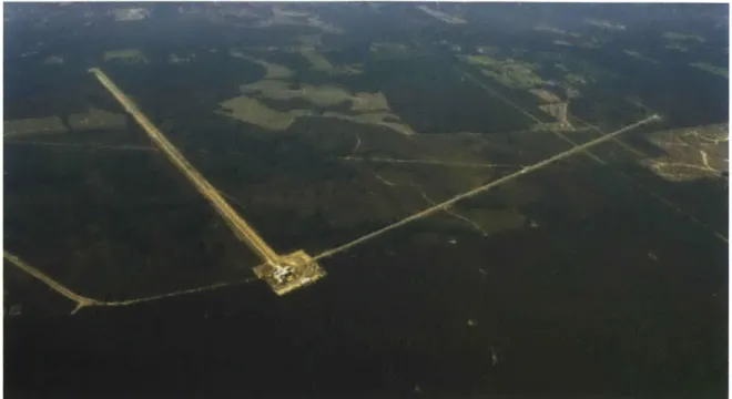
1-4 A photograph of the LIGO Livingston Observatory in Louisiana.

Cour-tesy of A ero D ata. . . . . 32

1-5 A top view of the optical layout of an Advanced LIGO observatory (not

to scale). A propagating GW passing through the observatory alters the differential length of the two 4 km perpendicular light storage arms. This differential length is measured with the amplitude of the light on

the photodetector. Adapted from

[3].

1-6 Projected displacement spectral density for the Advanced LIGO design

with contributing noise sources. The strain spectral density sensitivity is found by scaling the displacement down by 4000 m, the length of the interferometer arms. The measured Initial LIGO displacement is

1-7 Layout of the three cascading systems of seismic attenuation for

Ad-vanced LIGO's test masses: HEPI, a single stage active isolation sys-tem external to the vacuum chamber; The ISI, a two stage active and passive isolation system inside the vacuum chamber; and a quadruple pendulum, a passively isolating system whose bottom stage is a test

m ass. Adapted from [5, 6]. . . . . 37

1-8 The two stage active-passive Internal Isolation System (ISI). The ISI

is supported inside the vacuum system by HEPI. The ISI supports the

quadruple pendulum that suspends the ETM and ITM optics [3]. . . 37

1-9 Upconversion of seismic disturbances in Initial LIGO at the Hanford,

WA observatory during February 2006. Courtesy of Samuel Waldman. 39

2-1 _{Blue line: expected motion along the translational DOFs of the table}

from which the quadruple pendulum hangs. The rotational DOFs have similar numerical values, but in units of radians rather than meters

[4, 7]. Green line: the test mass requirement along the x DOF within the GW detection band. The pendulum must achieve more than six

2-2 (a): An illustration of the quadruple pendulum. It consists of two chains, a main chain (right) and a reaction chain (left). Stage 4 of the main chain is the interferometer optic. Three stages of cantilever springs provide vertical isolation. Sensor actuator devices (OSEMs) provide active damping and control in conjunction with an electro-static drive (ESD). The reaction chain is used as a seismically isolated actuation surface. (b): A photograph of a prototype quadruple pen-dulum at the Rutherford Appleton Lab in the UK. Stages 3 and 4 are stainless steel dummy stages whereas the production versions are fused silica glass. Stages 1 and 2 are almost entirely covered by the surrounding cage. The cage's purpose is to mount sensors, actuators, and to catch the stages. Copyright Science and Technology Facilities C oun cil. . . . . 49

2-3 The isolation performance for pendulums consisting of 1 through 4 stages, where the lowest stage is an optic. Each curve is a simulated transfer function between ground motion and the displacement of the

lowest stage of the pendulum along the interferometer axis. The triple and quadruple pendulum curves are simulations of actual Advanced

LIGO pendulum designs. The single and double pendulum curves are

illustrative exam ples. . . . . 51

2-4 A drawing of the working parts of an OSEM. The basic OSEM compo-nents consist of an LED, photodiode, and coil of wire. A flag mounted to a stage on the quadruple pendulum blocks part of the LED light and produces a position dependent signal from the photodiode. When a current is run through the coil an actuation force is produced on a permanent magnet mounted under the flag. Adapted from [8]. .... 53

2-5 The modeled frequency response of the stage 1 actuation including the current driver and a coil-magnet pair. The current driver has two poles

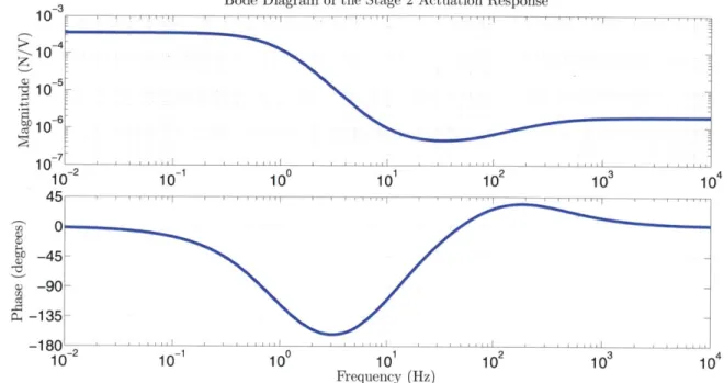
2-6 The modeled frequency response of the stage 2 actuation including the current driver and a coil-magnet pair. The current driver has three poles at 1 Hz, one pole at 325 Hz, three zeros at 10 Hz, and one zero at

60 H z [10]. . . . . 54

2-7 The modeled frequency response of the stage 3 actuation including the

current driver and a coil-magnet pair. The current driver has poles at

0.5 Hz, two at 200 Hz and zeros at 5 Hz and two at 20 Hz [11]. . . . . 54

2-8 A photograph of a prototype quadruple pendulum electrostatic drive (ESD) on the reaction chain bottom stage. Each quadrant has two

interlaced gold traces. A potential difference between the traces will

apply a force on the dielectric surface of the nearby test mass. . . . . 55

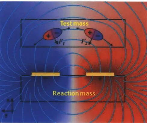
2-9 A diagram illustrating the working principle of the ESD. The upper

rectangle represents the test mass containing two polarized molecules; the lower rectangle represents the reaction mass bearing two electrodes.

The electric field lines are shown in cyan [12]. . . . . 56

2-10 The modeled dependence of the ESD coupling coefficient ae on the gap

between the test mass and stage 4 of the reaction chain [12]. . . . . . 57

3-1 The four system identification configurations of the quadruple

pendu-lum from which measurements are taken. The configuration on the left shows measurements being taken on the single pendulum of stage 4 while stage 3 is locked. The next shows measurements on the double

pendulum of the lower two stages, then the triple pendulum of the lower three stages, and finally the full pendulum. The sketched in eye balls indicate where measurements are taken. The fists indicate where

4-1 The solid line shows the values of the parameter uncertainty

sensitivi-ties in descending order (pj). The dashed line shows the squared length

of P up to its J"h component. The dashed line can be interpreted as the integral of the squared elements of the solid line. The dotted line

indicates that all parameters beyond j = n* = 8 in ]P are rejected. . . 81

4-2 The solid line shows the values of the measurement sensitivities in

descending order (4). The dashed line shows the squared length of

E, up to its ith component. The dashed line can be interpreted as

the integral of the squared elements of the solid line. The dotted line

indicates that all parameters beyond i = m* = 20 in 4 are rejected. . 81

4-3 Original quadruple pendulum model against the measured stage 1 pitch to pitch transfer function. The blue curve is the model, the red the

m easurem ent. . . . . 83

4-4 Model fit result, using all 47 measurements, against the measured stage

1 pitch to pitch transfer function. The blue curve is the model, the red

the m easurem ent. . . . . 84

4-5 Model fit result, using the selected 20 measurements, against the mea-sured stage 1 pitch to pitch transfer function. The blue curve is the

model, the red the measurement. . . . . 85

4-6 The solid line is the sum of the squared error at each iteration of the fitting routine when all 47 measurements are used. The dashed line is the sum of the squared error when only the selected 20 measurements

are used... ... 85

5-1 The Advanced LIGO displacement sensitivity from Figure 1-6 extended

5-2 A schematic diagram of the test mass (stage 4) positioning control loop. Actuation is applied on all four stages of the pendulum to control the position of the test mass, y, along the interferometer axis. The signals

u must be maintained within the l01V limit of the DAC. A1 to A4

represent the actuator dynamics. . . . . 89

5-3 The block diagram of the test mass positioning control loop. Actuation

is applied on all four stages of the pendulum to control the position of the test mass, y, along the interferometer axis. The signals u must be

maintained within the ±10 V limit of the DAC. . . . . 90

5-4 Amplitude spectra of the DAC voltages u8. . . . . 91

6-1 A block diagram of a modal damping scheme for the four x modes.

An estimator converts the incomplete sensor information into modal signals. The modal signals are then sent to damping filters, one for each mode. The resulting modal forces are brought back into the Cartesian coordinate system through the transposed inverse of the eigenvector matrix <b. Only stage 1 forces are applied for enhanced sensor noise

filtering to stage 4. . . . . 95

6-2 Left, the loop gain transfer function of an example 1 Hz modal oscillator

with its damping filter. Right, the root locus plot of the modal damping loop. The plant contributes the large resonant peak and 0 Hz zero, the damping filter contributes the remaining poles and zeros. All the damping loops have the same basic shape but are shifted in frequency

and gain (except the fixed frequency 10 Hz notch). . . . . 97

6-3 The components of the cost function (6.12) for the x DOF as a function

of R calculated by the optimization routine. At each value of R the closed loop system performance is simulated using the estimator design

6-4 An amplitude spectrum showing a simulation of the test mass displace-ment along the x DOF under the influence of the optimized modal

damping loop with R = 9 x 10-. The black dashed line is the sensor

noise and the green line is its contribution to the test mass displace-ment. The solid black line is the ground disturbance and the blue line is its contribution to the test mass displacement. The red line is the

uncorrelated stochastic sum of both contributions. . . . . 102

6-5 The dashed and dotted lines are the closed loop damping ratios as

a function of (,. The open loop mode frequencies are 0.440 Hz and

0.982 Hz. The shaded region represents the area beyond the critical

p o in t. . . . . 105

6-6 The dashed and dotted lines are the closed loop mode frequencies as

a function of (. The open loop mode frequencies are 0.440 Hz and

0.982 Hz. The shaded region represents the area beyond the critical

p oint. . . . . 106

6-7 The mode 1 closed loop damping ratio (CL,1 versus the reference

damp-ing ratios for both modes 1 and 2. Both reference dampdamp-ing ratios are less than or equal to the critical value (,,c = 0.3812. In this example

(CL,c = 0.4124. . . . . .. - - - . . .. - - - . . 108

6-8 The mode 2 closed loop damping ratio (CL,2 versus the reference

damp-ing ratios for both modes 1 and 2. Both reference dampdamp-ing ratios are less than or equal to the critical value (,c = 0.3812. In this example

(CL,c = 0.4124 . . . . .. . . . . . .. . -. . . . . .. - -. 109

6-9 The dashed, dotted, and thick solid lines are the closed loop damping

ratios as a function of (,. The open loop mode frequencies are 0.440 Hz,

0.982 Hz, 1.9873 Hz, and 3.3942 Hz. . . . . 111

6-10 The dashed, dotted, and thick solid lines are the closed loop mode

frequencies as a function of (,. The open loop mode frequencies are

6-11 The mode 1 closed loop damping ratio (CL,1 versus the reference

damp-ing ratios for modes 1, 2, 3, and 4. The (r,2,3,4 axis considers all (CL,1

values at (r,1 within the cube defined by (r,2 (r,2,3,4, (r,3 < (r,2,3,4,

(r,4 < (r,2,3,4. The (CL,1 value plotted represents the largest deviation

from (r,1, where the deviation is measured as

|C,-

deviation over the entire plot is 12%. . . . . 113

6-12 The mode 2 closed loop damping ratio (CL,2 versus the reference

damp-ing ratios for modes 1, 2, 3, and 4. The (r,1,3,4 axis considers all (CL,2 values at (r,2 within the cube defined by

Cr,i

(r,4 < r, 1,3,4. The (CL,2 value plotted represents the largest deviation from (r,2, where the deviation is measured as CL,2 - 1. The largest

(,,2

deviation over the entire plot is 15%. . . . . 113

6-13 The mode 3 closed loop damping ratio (CL,3 versus the reference

damp-ing ratios for modes 1, 2, 3, and 4. The (r,1,2,4 axis considers all (CL,3 values at (r,3 within the cube defined by

Cr,1

C,4

from (,3, where the deviation is measured as

|"

(,,3

deviation over the entire plot is 35%. . . . . 114

6-14 The mode 4 closed loop damping ratio (CL,4 versus the reference damp-ing ratios for modes 1, 2, 3, and 4. The (,1,2,3 axis considers all (CL,4

values at G,4 _{within the cube defined by (,1} G,1,2,3, r,2 < (,1,2,3 r,3 < (r,1,2,3. The (CL,4 value plotted represents the largest deviation from (,4, where the deviation is measured as C4 - 1|. The largest

d.,4

6-15 The response of stage 4 to an impulse at stage 1 along the x axis with

modal damping engaged. The damping values are set to the values

listed in Eqs. (6.29) to (6.32) so that each mode damps to in 10 s.

The solid red line is the response with the ideal unity feedback filters. The dashed blue line is the response with the filters designed in Section

6.2. The dotted lines represent the required decay amplitude for the

practical feedback. . . . . 115

7-1 Seismic disturbances at the Livingston, LA observatory, Nov. 21, 2009

measured with commercial Streckeisen STS-2 seismometers. Courtesy

L IG O L ab . . . . 122

7-2 Top level block diagram of adaptive modal damping applied to a

quad-ruple pendulum. The interferometer control is included for reference. 123

7-3 Signal flow block diagram inside the cost box. . . . . 124

7-4 Illustration of the modal bandpass filters. The blue line in the back-ground is a simulation of an example stage 1 displacement spectrum for a two mode system. The magnitude of this line is arbitrary. The dotted and dashed lines are the unitless bandpass filter transfer functions. 125

7-5 Simulated example of the response of an RMS filter with different time

constants. The blue trace in the background is the input to the filter, the dashed black and red solid lines are the outputs with different time

constants. . . . . 126

7-6 Example cost function employed by the adaptive modal damping method

for each mode. In this example, D = 94, Mo = 6, and ko = 100. . . . 129

7-7 Boundary layer separating the cost function space into slow and fast

7-8 Experimental Fabry-Perot cavity setup at MIT used to test the adap-tive modal damping technique. The input laser power is 10 mW, the power transmission coefficient of the triple pendulum test mass is 0.01 and the transmission coefficient of the quadruple pendulum test mass

is

5

7-9 This figure shows the response of the MIT setup to disturbances applied by shaking the table underneath the triple pendulum. The top half of

plot (a) shows the measured change in displacement between the two test masses due to the velocity of these disturbances shown in the bottom plot of (a). Plot (b) shows the measured power of the laser transmitted through the quadruple pendulum, which is proportional to the power resonant in the cavity between the test masses. Plot (c) shows the response of the adaptive damping gains. . . . 139

7-10 The steady state measured amplitude spectra of the output of the MIT

interferometer with varying amplitudes of seismic disturbance. These disturbances are applied by shaking the table supporting the triple pendulum and are designed to be flat in velocity between 1 Hz and

3 Hz and close to zero elsewhere. The disturbance signal comes from

filtering white noise through a bandpass elliptical filter. The modal adaptive damping is allowed to respond and settle to each amplitude

of seism ic disturbance. . . . . 141

8-1 _{Top level block diagram of the simulation used to investigate the}

influ-ence of adaptive modal damping on the sensitivity of Advanced LIGO to particular GW sources. . . . 144

8-2 Seismic disturbance and damping sensor noise included in the modal

8-3 Simulated example of relevant low and high noise terms relative to Advanced LIGO's nominal design sensitivity. The high upconverted seismic disturbance line is generated from large disturbances between

0 Hz and 4 Hz when damping is small. The upconversion results from

a simulated quadratic nonlinearity term in the behavior of the inter-ferometer with large displacements. . . . . 147 8-4 Effect of seismic disturbance on inspiral sensitivity as a function of

inspiral mass. The horizontal axis lists the mass of each object in a symmetric binary system. . . . . 152 8-5 Effect of damping noise on inspiral sensitivity as a function of inspiral

mass. The horizontal axis lists the mass of each object in a symmetric binary system . . . . 153 8-6 The inspiral volume for two 150 solar mass inspiraling black holes for

varying seismic amplitudes and damping levels. . . . . 154

8-7 Summary of inspiral volume results with and without adaptive modal damping. This data is listed in the last column of Tables 8.2 and 8.3. 156 8-8 Simulated interferometer sensitivity with the optimal modal damping

gains for the maximum seismic disturbance. . . . . 157 8-9 The solid black line is the Advanced LIGO sensitivity with the

max-imum seismic disturbance and optimal damping. The dotted black line is the sensitivity with the maximum disturbance and minimum damping. The dashed magenta line (courtesy Scott Hughes) is the characteristic signal produced by two inspiraling neutron stars of 1.4 solar masses each at a distance of 100 Mpc from the Earth. . . . . 158 8-10 The relative sensitivity of the Advanced LIGO detector to stochastic

gravitational waves at all frequencies. The listed energy densities, g,

List of Tables

2.1 The spectral limits on the motion of the test mass within the Ad-vanced LIGO GW detection band. The technical noise is restricted to contribute less than one part in ten to the overall motion of the test mass along the translational DOFs. Motion along the rotational DOFs is merely specified as an upper limit [13]. . . . . 47

5.1 The least squares DAC voltages i1, of each actuator and the probabil-ities p of saturating at the ±10 V limit. The probabilprobabil-ities refer to each

DAC sam ple tim e. . . . . 92

8.1 Adaptive modal damping cost function parameters. . . . . 154

8.2 Optimal damping values determined by the selected cost functions. The last column lists the inspiral volume for two 150 solar mass black holes. The percentage of the inspiral volume to the best case volume is given in parenthesis. . . . . 155 8.3 Inspiral results for the maximum disturbance with the maximum and

minimum damping levels. The last column lists the inspiral volume for two 150 solar mass black holes. The percentage of the inspiral volume to the best case volume is given in parenthesis. . . . . 156

8.4 Advanced LIGO stochastic sensitivity results from the simulation. The last row is the case of optimal damping with the maximum seismic

Chapter 1

Introduction

The remaining years of this decade promise to be an exciting time for gravitational wave astronomy. Current upgrades to existing gravitational wave observatories such as the Laser Interferometer Gravitational-Wave Observatory (LIGO) are likely to make direct observations of these waves from massive compact events in space possible for the first time. For some of these events, such as black hole mergers and early universe processes, gravitational waves may be the only detectable radiation emitted. For others such as supernovae, these waves can augment electromagnetic observations, providing ever deeper astrophysical understanding.

Gravitational waves have not yet been directly observed because they interact so weakly with any possible detector design. Consequently, the science available to current (and foreseeable future) observatories is limited by many sources of noise. One class of these noise sources for ground based detectors such as LIGO consists of non-stationary disturbances coming through the ground. These disturbances are con-stantly evolving in time depending on weather, tides, and man-made activities. Many active control loops are involved to compensate for these disturbances to maintain the detectors at a set operating point. The main contributions in this thesis target the development of an adaptation algorithm to optimize certain control loops for the observation of astrophysical sources of gravitational waves.

1.1

Behavior of Gravitational Waves

Gravitational waves (GWs) are currently undetected phenomena predicted to exist

by Einstein's Theory of General Relativity. In this theory accelerating mass produces

GWs in a manner analogous to the way accelerating charges produce electromagnetic waves. Additionally, GW's interaction with surrounding space is incredibly weak. Only the most massive and violent events in the universe such as supernovae and collisions of black holes or neutron stars produce GWs strong enough to consider detecting [1].

The effect of GWs is quite different from electromagnetic waves. As they prop-agate they compress and stretch space. Consider the ring of particles in Figure 1-1 below. If the axis of propagation is perpendicular to the page then the shape of space is altered in the plane of the page, perpendicular to propagation. Two perpendicular axes in this plane simultaneously have opposite effects; one is stretched while the other is compressed.

y

h+®:xQQ

CS~O

time

hxOOO

₎

Figure 1-1: Effect of a GW on a ring of particles. The top half shows the effect of a wave polarized with axes, x and y, parallel to the vertical and horizontal axes of the page. The lower half shows the effect of a wave polarized at 450 relative to the upper wave. Space is alternately compressed and stretched along the wave's x and y axes

as it propagates through the plane [1].

The figure shows two different polarizations of a GW [14, 15]. Polarization is defined as the tilt of the plane wave's x and y axis relative to the observer. The upper half of the figure, h+, is a case when the polarization is parallel with the vertical and horizontal axes of the page. The lower one is a case when the polarization is tilted

be planar.

The stretching of space is similar to the concept of mechanical strain in that it is a proportional effect. If two objects are far apart, the distance between them will change more than for two objects that are close together. The amount of strain produced by a GW, h, is proportional to the strength of the wave. For a GW of strength h, the specified distance L is altered by AL = hL. For more details on GWs and associated general relativity see [14, 15].

1.2

Sources of Gravitational Waves

Sources of GWs that are expected to be strong enough for detection by current and upcoming observatories include coalescing compact binaries, pulsars, supernovae, and a stochastic background. These sources encode in their waves rich information about general relativity and astrophysics. A non-exhaustive summary of these sources and the scientific knowledge they encode in their waves is presented in this section. More information can be found in [16, 17, 18].

1.2.1 Binary Inspirals

A binary inspiral is a coalescing pair of compact, massive objects such as black holes

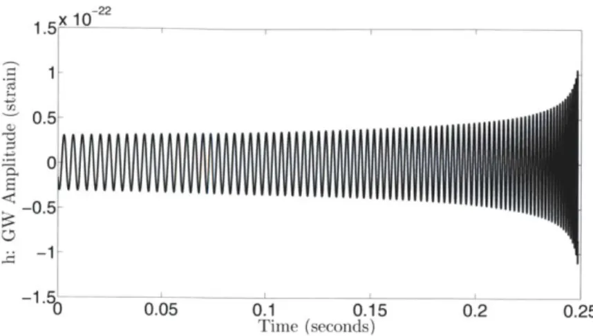
and neutron stars. Such events begin with the objects orbiting around their common center of mass. The orbital distance and period gradually decay due to energy loss through the emission of gravitational radiation. The pair begins spiraling into the center of mass and the GW signal increases both in frequency and amplitude creating a chirp-like signal. Finally both objects crash into each other emitting a final burst of gravitational radiation. Figure 1-2 plots the waveform for last 0.25 seconds of two

1.4 solar mass inspiraling neutron stars.

Inspirals are a potentially rich source of information. Their GWs encode informa-tion about their populainforma-tion in the universe and mass and spin properties. The tidal disruption of a neutron star merging into a black hole produces information on the neutron star matter's equation of state of which there is still much uncertainty. The

1 .5 -- - - 0.5-0 -0.5--. 0 0.05 0.1 0.15 0.2 0.25 Time (seconds)

Figure 1-2: The last quarter second of an inspiral waveform for two 1.4 solar mass neutron stars 100 Mpc from Earth.

merging of two black holes creates the most extreme warping of space time, providing detailed information on the as yet untested nonlinear strong field dynamics of general relativity.

1.2.2

Pulsars

Pulsars are rotating neutron stars that emit GW radiation due to their rotation. This is another mechanism for neutron stars to emit observable gravitational radiation. Spherical symmetry prevents wave emission, but if the star is slightly asymmetric (its ellipticity) and rotating quickly enough, then waves strong enough to observe from Earth may be produced at twice the pulsar's rotational frequency.

Long term observations of these waves as the Earth revolves around the sun reveal to high precision the location in the sky of the pulsar, which enables the blending of electromagnetic observations. Comparison's between GW and electromagnetic observations can divulge inhomogeneities in the density of the pulsar and its ellipticity. GWs can also carry more detailed information about the star's structure such as the properties of its crust, crust-core interactions, viscosity, etc. There is also the possibility of observing a so-called r-mode oscillation in fast spinning stars, which is an unstable oscillation in the GW induced flow of material within the star. This oscillation contributes to the strength of the waves, thus enhancing the oscillation further until dissipative forces bring it to an equilibrium.

1.2.3

Bursts

Bursts represent a class of cosmic events characterized by high energy output on short time scales. One example is the type-II supernova, which is the explosive death of a massive star and the subsequent collapse of the core to a neutron star or black hole. The exact evolution of a supernova is not well known, so this source provides an excellent opportunity to expand scientific knowledge of such phenomena. Many of these events have already been observed through neutrino and electromagnetic emissions. Merging these observations with concurrent GWs would produce a more complete picture of these events than any that has been achieved to date. GW emission requires the collapse of the stellar core to have spherical asymmetry, however it is believed this is usually the case. For example, if the core is spinning its collapse will not be symmetric and strong waves can be produced. Since these events lead to neutron stars and black holes there is a considerable opportunity to study these

compact objects just as they are born in ways that are not achievable otherwise. Gamma ray bursts include another set of possible sources in this class. These events emit strong bursts of gamma rays over a period of a fraction of a second to

100 seconds. They are observed approximately once per day by dedicated satellites,

in particular by the Swift mission [19]. The specific triggers for gamma ray bursts are not well formalized, but it is believed they come from a variety of sources such as supernovae, accretion around a black hole, and the merger of compact binary objects.

1.2.4

Stochastic Background

Stochastic background radiation encompasses a final class of GWs. The background could consist of either an incoherent superposition of many discrete weak sources or primordial radiation from very early times following the Big Bang. The stochastic signals are expected to be broadband and extremely weak. They are generally mod-eled as being isotropic, stationary, and Gaussian, though these assumptions are not necessarily true. There are many ways to break the anisotropy assumption. A simple example is for a background dominated by discrete sources in the Milky Way, such

as binary white dwarfs. Since the galaxy is not spherical the strongest signals would point towards the bulk of the Milky Way in the sky. The stationary assumption is reasonable given that the universe evolves on cosmological timescales that are much greater than the anticipated lifetime of GW observation. The Gaussian assumption is reasonable in particular for a background dominated by early universe radiation.

Current understanding of the nature of this background is rather poor. It is unknown for instance which of the two stochastic components will dominate, the pri-mordial radiation or the superposition of discrete sources. Conversely however, there is room for large gains in knowledge. The primordial radiation, if visible, will contain

information about the universe as early as 10-22 s after the Big Bang. In comparison,

our current earliest view of the universe comes from Cosmic Microwave Background Radiation (CMBR) originating at 10' years after the big bang [20]. Observations of the stochastic background will help answer many of these unknowns.

1.3

LIGO

For the first time the direct detection of GWs may now be possible due to the work of observatories such as the Laser Interferometer Gravitational-Wave Observatory

(LIGO) [3, 21, 22]. To date, no direct detections of GWs have been made due to

the weak interactions of gravitational radiation. A typical wave produced from such

powerful sources as described in section 1.2 is expected to induce a strain of only 10-22,

about 104 times smaller than the diameter of a proton for the 4 km observation paths

used in LIGO. Earth-based detectors, such as LIGO, have the added complication of natural and man-made noise traveling through the ground. Nearly all the work of these detectors up to this point is focused on developing ways to amplify the signal and reduce sources of noise that will wash out these infinitesimally small signals.

In order to bring observations of gravitational waves into the realm of regular astronomy, the second generation of LIGO known as Advanced LIGO [3] is currently under construction. Advanced LIGO increases the sensitivity of the first generation of LIGO, known as Initial LIGO by tenfold over a broad frequency band. This increases

the volume of space visible to LIGO by a factor of 1000, which brings the expected GW detection rate from about once is a handful of years to as much as once a day.

1.3.1

Advanced LIGO Layout

Advanced LIGO installation is currently underway within the existing LIGO vacuum envelopes at the two LIGO sites in Livingston, Louisiana and Hanford, Washington. See Figures 1-3 and 1-4 for photos of these observatories. To improve upon the Initial LIGO sensitivity nearly all hardware with the exception of the vacuum system itself will be upgraded. These systems include seismic isolation, optics, and lasers [3].

Figure 1-3: A photograph of the LIGO Hanford Observatory in Washington State [2].

Each Advanced LIGO detector consists of a Michelson interferometer with 4 km long Fabry-Perot cavities in each perpendicular arm, used to measure the differential arm length caused by the passing wave. A long arm length was chosen in order to maximize the length change induced by the strain of the wave. The interferometer is housed in a vacuum envelope evacuated to about 10-' Torr to prevent interference from gas particles.

Figure 1-5 shows the schematic diagram of these interferometers. The exact details of how these detectors work are rather complicated, but the essential principles can

Figure 1-4: A photograph of the LIGO Livingston Observatory in Louisiana. Courtesy of Aero Data.

be described as follows. A laser injects 1064 nm (infrared) light into a beam splitter that splits the light into the two orthogonal arms. A Fabry-Perot cavity in each arm of the Michelson, comprising optics referred to as an input test mass (ITM) and an end test mass (ETM), stores the laser light to increase the phase sensitivity of the interferometer. The test masses are suspended as pendulums in order to isolate them from ground motion and act as free test particles, such as those in the rings of Figure

1-1. A photon will make approximately 100 round trips between these optics in order

to amplify the length measurement of each arm. The light then recombines at the beam splitter and continues on to a photodetector. Measuring the intensity of the light at this photodetector provides a measure of the phase difference of the light in each arm, and thus the differential length [1].

The purpose of multiple observatories is motivated by several factors. One is to locate which part of the sky the GW came from and determine its polarization. Another is to create veto scenarios so that GWs can be distinguished from local noise sources such as a heavy truck driving down a nearby road. A GW of cosmic origin should be present coincidentally at both sites whereas the truck will not.

I

Input Mode Cleaner

Beam

Splitter-Laser

Power Recycling

Mirror

End Test Mass

Input Test Mass

Compensation

Plate

Signal

Mirror

*g

+-

Photodetector

- Output Mode Cleaner

Figure 1-5: A top view of the optical layout of an Advanced LIGO observatory (not to scale). A propagating GW passing through the observatory alters the differential length of the two 4km perpendicular light storage arms. This differential length is measured with the amplitude of the light on the photodetector. Adapted from [3].

1.3.2

Sensitivity Limiting Noise Sources

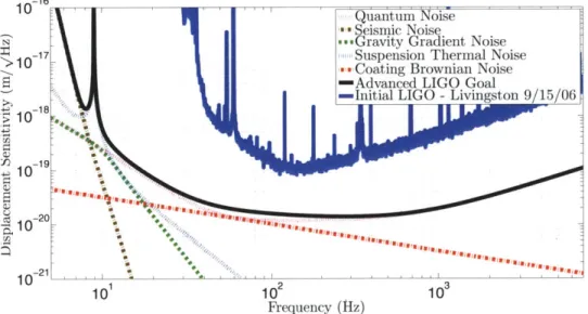
In order to make the detectors sensitive enough to see GWs, many different sources of noise and disturbances in the LIGO detection band (10 Hz to 8 kHz) have to be eliminated or reduced. The dominating sources are categorized into seismic, gravity gradients, thermal, and quantum noise. Quantum noise consists of both radiation pressure and shot noise. Each source contributes to specific parts of the spectrum

[3]. Figure 1-6 shows each one relative to the Advanced LIGO design sensitivity. The

measured Initial LIGO sensitivity from the Livingston Observatory is included for reference.

10-1 1016uantum Noise

Seismic Noise

-- Gravity Gradient Noise

-17 -Suspension Thermal Noise

'10

- _{.Coating Brownian Noise}

-Advanced LIGO Goal

-Initial LIGO - Livingston 9/15/06

-4-D -18 10 10-10 -20 ~ -21 10 ' 2 3 10 10 10 Frequency (Hz)

Figure 1-6: Projected displacement spectral density for the Advanced LIGO design with contributing noise sources. The strain spectral density sensitivity is found by scaling the displacement down by 4000 m, the length of the interferometer arms. The measured Initial LIGO displacement is plotted for reference. Adapted from [3, 4].

Seismic disturbances dominate at frequencies below about 10 Hz. The term seismic is used to collectively refer to all sources coming through the ground. These sources include actual seismic motion from tectonic plates and volcanic activity. However, it also includes noise from ocean waves crashing onto the shores as well as man-made activity. A nine order of magnitude attenuation is needed to meet the Advanced

LIGO sensitivity requirement at the 10 Hz start of the GW detection band.

and a possible contribution from gravity gradient noise. Radiation pressure noise is the disturbance from the momentum transfer of random numbers of photons from the

interferometer laser reflecting off the test masses. It scales with the square root of the laser power [23]. The thermal noise in this band is associated with the mechanical dissipation of the test mass suspension systems. Thermal energy in the materials making up the suspensions (particularly the silica fibers supporting the test masses) couple to the motion of the test mass along the interferometer axis. Gravity gradient noise refers to classical (as opposed to relativistic) fluctuations in the local gravi-tation field from variations in the distribution of nearby mass, particularly density fluctuations in the local ground.

From about 40 Hz to 200 Hz radiation pressure combines with shot noise and ther-mal noise in the test mass optical coatings to limit the sensitivity. Radiation pressure and shot noise are both quantum noises associated with the random distribution of discrete photons in the laser light. Radiation pressure physically moves the test masses as described above, whereas shot noise is a sensing problem. The random number of photons at any given moment falling on the photodetector measuring the interferometer output generates the shot noise contribution. It scales with the inverse square root of the laser power. Consequently, there is a fundamental design trade-off when choosing the laser power since radiation pressure scales with the square root of the laser power. Frequency dependent squeezing technology is currently under development to improve upon this quantum noise trade-off [24]. The optical coating thermal noise has the same process as the suspension thermal noise except that here the source is in the coating on the test mass surface. Beyond 200 Hz shot noise will be the sole dominating noise.

1.3.3

Seismic Isolation Systems

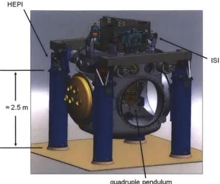
Advanced LIGO requires the installation of sophisticated seismic isolation systems to reach design sensitivity in the seismic and thermal noise dominated band of the spectrum. This isolation is achieved with three cascading systems. For the test masses, where the noise contributions are most critical, these systems encompass a

total of seven stages of both passive and active isolation. Figure 1-7 is an illustration of how the three systems fit together in the vacuum chambers that house the test masses. This section focuses on these particular test mass systems. Similar systems with fewer stages exist for many of the auxiliary optics within the interferometer [25].

The first system, known as the Hydraulic External Pre-Isolator (HEPI), functions outside the vacuum chambers that house the test masses and internal isolation sys-tems. HEPI is a single stage that senses and actively removes ground motion by about an order of magnitude between the frequencies of 0.1 Hz to 10 Hz. Its specifi-cations call for actuation in all six degrees of freedom (DOFs), force generation up to 2000 N, a range of t1mm in translation, +1 mrad in rotation, and a noise floor no greater than 10-9 m//Hz at 1 Hz. The actuation is applied to the four corners of the support tubes that carry the internal seismic isolation systems. Bellows allow the motion to be transmitted to the inside of the vacuum chamber. HEPI has in-ertial and displacement sensors which feedback to collocated laminar flow hydraulic actuators. Seismometers placed nearby on the ground further enhance isolation with feedforward control [3, 5].

The second system, known as the Internal Seismic Isolation (ISI) system is shown in a detailed drawing by Figure 1-8. It supports the suspensions inside the chambers and is directly supported by HEPI. It is a two stage system providing both active and passive isolation. The ISI has inertial and displacement sensors that feedback to electromagnetic actuators to provide active isolation from about 0.2 Hz to 30 Hz. The two stages are suspended by cantilever springs which provide passive isolation beyond the bandwidth of the active isolation control. Overall, the ISI isolates by about a factor of 300 at 1 Hz and 3000 at 10 Hz [3, 5].

The second stage of the ISI is equipped with an optical table from which a passively isolating test mass suspension hangs. These suspensions are chains of four stages hanging from each other, where the bottom stage is an interferometer optic serving as a test mass. The test mass suspensions are known as the quadruple pendulum. The quadruple pendulum is describe in detail in Chapter 2.

HEP

' ISI

I 2

~2.5 m

quadruple pendulum

Figure 1-7: Layout of the three cascading systems of seismic attenuation for Advanced LIGO's test masses: HEPI, a single stage active isolation system external to the vacuum chamber; The ISI, a two stage active and passive isolation system inside the vacuum chamber; and a quadruple pendulum, a passively isolating system whose

bottom stage is a test mass. Adapted from [5, 6].

Stage 2 - Seismometer

Stage 1

Stage 0 _SpringsBlade

Figure 1-8: The two stage active-passive Internal Isolation System (ISI). The ISI is supported inside the vacuum system by HEPI. The ISI supports the quadruple

isolation is achieved with simpler versions of the aforementioned systems, generally

with fewer stages. Details of these systems can be found in reference [25].

1.3.4

Problems and Challenges

To measure the weakly interacting gravitational waves, LIGO's test masses must have a minimum relative displacement spectral density less than 10-19 m/ /Hz between

10 Hz and 10 kHz. This sensitivity is realized at the low end of LIGO's spectrum

through the advanced isolation systems described in Section 1.3.3. These systems have many coupled degrees of freedom that must be controlled to properly steer the test masses. LIGO requires that the overall relative root mean square (RMS) displacement and orientation between the test masses be less than 10-15 m and 10-9 rad respectively

[26] as a result of the fact that the interferometer's sensitivity to higher order nonlinear

terms increases with large motions of the test masses and isolation systems. These nonlinearities cause the generally low frequency ground vibrations to upconvert to frequencies where LIGO hopes to measure GWs. Many of the nonlinearity sources are either not measured or poorly understood, preventing their electronic subtraction from the interferometer's output. Some of the known or suspected sources result from laser light scattering off the walls of the interior vacuum system, laser light clipping from falling off the optics, the approximately quadratic nature of the interferometer output, higher order dynamics in the isolation systems, nonlinear actuator responses, and creak (sliding dislocations) in the materials of the isolation systems.

Additionally, the seismic disturbances the LIGO observatories experience is not constant in time. The magnitude of the noise changes depending on weather, earth-quakes, and highly variable man-made (anthropogenic) disturbances. Ideally, all the control loops would be designed with sufficiently large gains to keep the test masses

within an RMS of 10-5 m and 10-9 rad during the worst case seismic events. In

practice however, non-negligible sensor noise exists in many of the feedback control loops, limiting these gains. Therefore it is likely that purely linear control of the interferometer will not provide optimal GW sensitivity for all seismic disturbances.

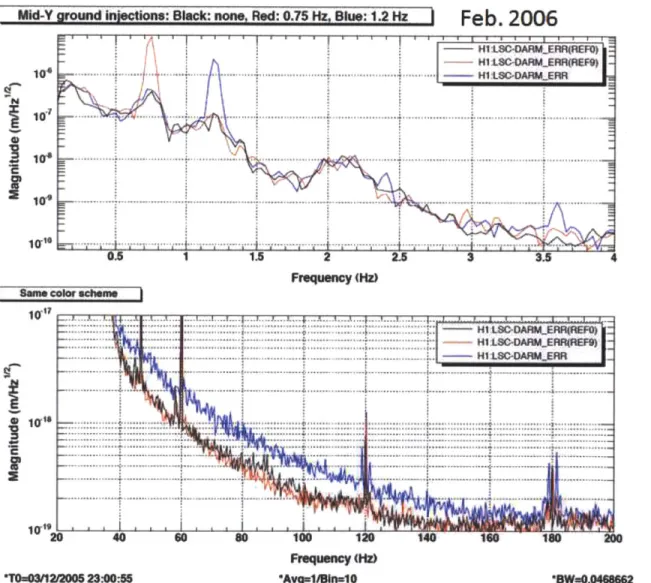
1-9 illustrates an example of moderately large low frequency seismic disturbance

up-conversion at the Hanford Observatory during February of 2006. The top plot shows different cases of disturbances between 0.1 Hz and 4 Hz. The lower plot shows the resulting interferometer displacement sensitivity between 20 Hz and 200 Hz. In this case upconversion was most apparent for the disturbance at 1.2 Hz. Historically, the largest seismic disturbances experienced by Initial LIGO would move the interfer-ometers so far beyond their linear range that they would go off-line until the period passed.

Mid-Y ground inec : Black: non, Red: 0.75 Hz Blue: 1.2 Hz

Nr

M

Feb. 2006

-HaSC-~DA1RM.AEF)

- H... -DA .E-R

Frequency

-TOananosas5 2:00:56 -Avgeniln=10 -sW.0460sess

Figure 1-9: Upconversion of seismic disturbances in Initial LIGO at the Hanford, WA

observatory during February 2006. Courtesy of Samuel Waldman.

To date, LIGO has devoted much effort to optimize the design of control ioops that

l

position the interferometer's many coupled degrees of freedom while rejecting seismic disturbances with the minimal amount of process noise. These control loops were designed with many types of methods including traditional loop shaping techniques, feedforward control, and modal damping [27, 4, 28, 29]. Certain adaptation tech-niques have been explored as well. Driggers et al [27] explored adaptive feedforward cancellation of seismic disturbances and Zuo [30, 31, 32] explored adaptive feedback control of isolation systems with unknown or time-varying plant parameters. Refer-ence [31] develops the concept of model reaching adaptive control. It improves upon model reference adaptive control by defining a goal for the system's dynamics, rather than its output. This change eliminates the need to measure ground disturbances. Reference [32] employs a frequency shaped sliding control method to robustly handle unknown or time varying system parameters.

1.4

Proposed Adaptive Approach for LIGO

Sus-pensions

Previous adaptive feedback work focused on unknown or time varying isolation table parameters. It did not go as far as considering the pendulums or show how the control or seismic disturbances influenced the output of the interferometer. At this point in Advanced LIGO's development, the pendulums are well understood and their parameters are static. Adaptive feedforward work did consider the interferometer output under changing seismic conditions, but the adaptation was limited to time scales longer than 10 minutes and it can be very computationally intensive for good performance.

Additional gains could be made with adaptive feedback control on the pendulums that takes directly into account the interferometer performance and unique aspects of these pendulums. Such a controller would adapt its parameters in real-time in some optimal way to balance the trade-off between rejecting non-stationary seismic disturbances and the interferometer's sensitivity to upconversion. A need also remains

to define the optimal trade-off directly in terms of LIGO's science goals. Adaptive modal damping is developed to implement this real-time automatic tuning for the case of the local damping of the quadruple pendulums, which is one component of the interferometer's overall feedback control architecture. However, similar adaptive methods are applicable to other control components such as test mass angular control, control of auxiliary optical cavities, and the isolation loops of the seismic systems.

Local damping refers to any control strategy used to reduce or 'damp' the large amplitude displacements of the pendulums induced by the residual seismic distur-bances amplified by high quality factor mechanical resonances. The proposed strat-egy, adaptive modal damping, incorporates a modal damping scheme enveloped by an adaption algorithm that adjusts the amount of damping applied to each mode in response to changing seismic disturbances. Modal damping is a convenient way to decouple the modes of vibration so they can be damped independently. Since each mode responds as a simple second order system, the design of each mode's com-pensator is minimally complex. As a result, it is relatively easy to find an optimal trade-off between damping and noise amplification for each mode. This trade-off is defined in terms of LIGO's sensitivity to the astrophysical sources of GWs listed in Section 1.2. The adaptive part of the control monitors the amplitude of each mode's response and scales the feedback gains of the compensators in real-time. More gain is chosen when a modal signal increases in amplitude and less gain when it decreases. The control also switches its adaptation rates for quick, coarse responses to sudden disturbances and slow, precise responses to steady disturbances.

1.5

Thesis Overview

The remaining chapters of this thesis support the main contributions of applying adaptive modal damping to the Advanced LIGO quadruple pendulums. Chapter 2 describes the design and requirements of the quadruple pendulum used to isolate and support the Advanced LIGO test masses. Chapter 3 describes the derivation of a model of the quadruple pendulum's equations of motion and the system