An adaptive space-time discontinuous Galerkin method for reservoir flows

(1)

An adaptive space-time discontinuous Galerkin

method for reservoir flows

by

Yashod Savithru Jayasinghe

M.Eng., University of Cambridge (2013) S.M., Massachusetts Institute of Technology (2015) Submitted to the Department of Aeronautics and Astronautics

in partial fulfillment of the requirements for the degree of Doctor of Philosophy in Computational Science and Engineering

at the

MASSACHUSETTS INSTITUTE OF TECHNOLOGY June 2018

c

Author . . . . Department of Aeronautics and Astronautics

May 24, 2018 Certified by . . . . Thesis Supervisor: David L. Darmofal Professor of Aeronautics and Astronautics Certified by . . . . Thesis Committee Member: Steven R. Allmaras Research Engineer of Aeronautics and Astronautics Certified by . . . . Thesis Committee Member: Ali H. Dogru Saudi Aramco Fellow Certified by . . . . Thesis Committee Member: Youssef M. Marzouk Professor of Aeronautics and Astronautics Accepted by . . . .

Hamsa Balakrishnan Associate Professor of Aeronautics and Astronautics Chair, Graduate Program Committee Accepted by . . . .

Nicolas Hadjiconstantinou Professor of Mechanical Engineering Co-director, Computational Science and Engineering

(2)

(3)

An adaptive space-time discontinuous Galerkin method for

reservoir flows

by

Yashod Savithru Jayasinghe

Submitted to the Department of Aeronautics and Astronautics on May 24, 2018, in partial fulfillment of the

requirements for the degree of

Doctor of Philosophy in Computational Science and Engineering

Abstract

Numerical simulation has become a vital tool for predicting engineering quantities of interest in reservoir flows. However, the general lack of autonomy and reliability prevents most numerical methods from being used to their full potential in engineering analysis. This thesis presents work towards the development of an efficient and robust numerical framework for solving reservoir flow problems in a fully-automated manner. In particular, a space-time discontinuous Galerkin (DG) finite element method is used to achieve a high-order discretization on a fully unstructured space-time mesh, instead of a conventional time-marching approach. Anisotropic mesh adaptation is performed to reduce the error of a specified output of interest, by using 𝑎 𝑝𝑜𝑠𝑡𝑒𝑟𝑖𝑜𝑟𝑖 error estimates from the dual weighted residual method to drive a metric-based mesh optimization algorithm.

An analysis of the adjoint equations, boundary conditions and solutions of the Buckley-Leverett and two-phase flow equations is presented, with the objective of de-veloping a theoretical understanding of the adjoint behaviors of porous media models. The intuition developed from this analysis is useful for understanding mesh adaptation behaviors in more complex flow problems. This work also presents a new bottom-hole pressure well model for reservoir simulation, which relates the volumetric flow rate of the well to the reservoir pressure through a distributed source term that is independent of the discretization. Unlike Peaceman-type models which require the definition of an equivalent well-bore radius dependent on local grid length scales, this distributed well model is directly applicable to general discretizations on unstructured meshes.

We show that a standard DG diffusive flux discretization of the two-phase flow equations in mass conservation form results in an unstable semi-discrete system in the advection-dominant limit, and hence propose modifications to linearly stabilize the discretization. Further, an artificial viscosity method is presented for the Buckley-Leverett and two-phase flow equations, as a means of mitigating Gibbs oscillations in high-order discretizations and ensuring convergence to physical solutions.

(4)

compress-ible two-phase flow problems in homogeneous and heterogeneous reservoirs. Compar-isons with conventional time-marching methods show that the adaptive space-time DG method is significantly more efficient at predicting output quantities of interest, in terms of degrees-of-freedom required, execution time and parallel scalability. Thesis Supervisor: David L. Darmofal

Title: Professor of Aeronautics and Astronautics Thesis Committee Member: Steven R. Allmaras

Title: Research Engineer of Aeronautics and Astronautics Thesis Committee Member: Ali H. Dogru

Title: Saudi Aramco Fellow

Thesis Committee Member: Youssef M. Marzouk Title: Professor of Aeronautics and Astronautics

(5)

Acknowledgments

I would like to express my sincere gratitude to all those who have helped, in numerous ways, to make this research study and thesis possible.

First and foremost, I would like to thank my advisor, Prof. David Darmofal, for giving me the opportunity to be a part of his research group, and for his consistent guidance, inspiration and encouragement throughout my graduate study. His insights, critiques and constructive feedback have been vital to the progress of this work. I would also like to thank Dr. Steven Allmaras for his valuable feedback and advice throughout my time at MIT, and for his dedication to the weekly meetings despite being three time zones away. The long chains of emails and discussions we have had about adjoints, boundary conditions and stability have taught me a lot on the subtler aspects of CFD analysis. Dr. Marshall deserves acknowledgement for his significant contributions to the two research codes developed and used by our group, ProjectX and SANS, and for patiently teaching us the ways of writing good code (with unit-tests of course). His vast programming experience and unparalleled availability for debugging, brainstorming and discussing various topics definitely made my graduate life a lot easier. I would also like to thank Nick Burgess and Eric Dow for their valuable input and perspectives from the industry at the weekly meetings, which helped shape the course of this thesis work. I would also like to thank the other members of my thesis committee, Dr. Ali Dogru and Prof. Youssef Marzouk, for their feedback on this thesis work. I’m also grateful to Prof. Abbas Firoozabadi and Prof. Qiqi Wang for reading the initial drafts of this thesis.

This work would have not been possible without the efforts and contributions of the entire ProjectX/SANS teams, both past and present. I would specifically like to thank Arthur, Ben, Carmen, Cory, Hugh, Philip and Shun for their contributions to SANS, and for being a passionate and helpful group of colleagues over the past few years. Masa also deserves recognition for laying down the foundations of the adaptive framework that is used in this work. I would also like to thank all the ACDLers for creating a productive and friendly working environment, including my fellow system

(6)

administrators, Chaitanya and Chi, for their support in setting up computers, moving clusters, and helping with all the other sysadmin things that kept the computational resources in the lab running smoothly. Being an ACDL sysadmin was truly a great learning experience outside research. Furthermore, I would also like to thank Beth, Jean, Kate, Meghan and Robin for their help with scheduling meetings, making travel arrangements and all the other important administrative tasks.

Outside the lab, I’m deeply grateful to Charith, Maleen, Sandamali, Nawodya, Prashan, Thulith, Tharanga, and Chamithri for making my life in Boston fun and colorful, with all the game-nights, movies and hikes. Thank you Thanuja, for the Skype calls from the other end of the world, and for being a great friend all these years. Narmada, no words will do justice for the love, support, and wonderful memories you have given me over the past five years. Thank you for making MIT feel home.

Lastly, I would like to thank my parents and sister for their unconditional love and constant support, without which I would never have gotten this far. I’m forever indebted for all the sacrifices you have made to help me pursue my goals. I wish all of you the best of happiness and health.

This research was supported through a Research Agreement with Saudi Aramco, a Founding Member of the MIT Energy Initiative (http://mitei.mit.edu/), with tech-nical monitors Dr. Ali Dogru and Dr. Eric Dow.

(7)

List of Figures

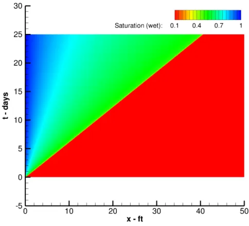
1-1 Space-time mesh for an elastodynamics problem (Hughes [76]) . . . . 21 1-2 Illustration of different space-time meshes . . . 21 1-3 General outline of the adaptation framework . . . 23 2-1 Mesh metric-field duality (Modisette [99]) . . . 45 2-2 Example split configurations with associated metric tensors (Yano [137]) 47 3-1 Schematic of space-time domain Ω . . . 53 3-2 Primal solution of Buckley-Leverett problem using a second-order

space-time DG method with 750,000 DOF. . . 62 3-3 Comparison of space-time DG (solid lines) and exact (dashed lines)

primal solutions at different times. . . 62 3-4 Primal characteristics of the Buckley-Leverett problem entering the

shock (blue region) or exiting the top (grey region) and right (red region) boundaries. . . 63 3-5 Exact adjoint solution for output 𝐽𝑇. . . 65

3-6 Numerical adjoint solution for output 𝐽𝑇 from a second-order

space-time DG method with 750,000 DOF. . . 66 3-7 Comparison of space-time DG (solid lines) and exact (dashed lines)

adjoint solutions at different times, for output 𝐽𝑇. . . 66

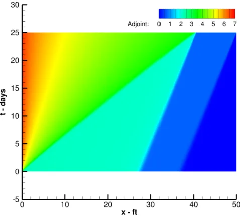
3-8 Exact adjoint solution for output 𝐽 . . . . 68 3-9 Numerical adjoint solution for output 𝐽 from a second-order space-time

(12)

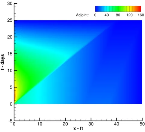
3-10 Comparison of space-time DG (solid lines) and exact (dashed lines) adjoint solutions at different times, for output 𝐽 . . . . 69 3-11 Numerical adjoint solution 𝜓𝑤 for output 𝐽 from a second-order

space-time DG method with 750,000 DOF per state variable. . . 78 3-12 Numerical adjoint solution 𝜓𝑛 for output 𝐽 from a second-order

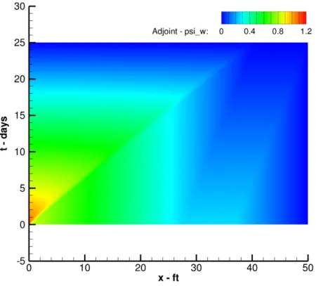
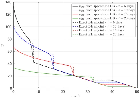
space-time DG method with 750,000 DOF per state variable. . . 78 3-13 Space-time contour plot of 𝜓𝐵𝐿 = 𝜌𝑤𝜓𝑤 − 𝜌𝑛𝜓𝑛, computed from the

numerical adjoint solutions. . . 79 3-14 Comparison of 𝜓𝐵𝐿with the exact Buckley-Leverett adjoint at different

times. . . 79 4-1 Outline of linearized analysis for deriving upwinding modifications . . 83 4-2 Generalized eigenvalues of a DG P0 discretization of the linearized

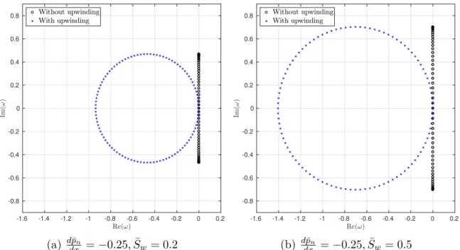
two-phase equations with periodic BCs, for different mean solutions . 93 4-3 Generalized eigenvalues of a DG P1 discretization of the linearized

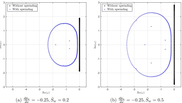
two-phase equations with periodic BCs, for different mean solutions . 93 4-4 Generalized eigenvalues of a DG P1 discretization of the linearized

two-phase equations with Dirichlet BCs, for different mean solutions . 95 4-5 Generalized eigenvalues of a DG P1 discretization of the nonlinear

two-phase equations with Dirichlet BCs, evaluated at a P1 L2_{-projection of}

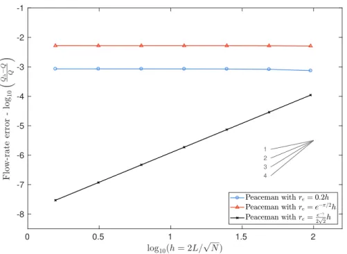
the mean solution . . . 95 5-1 Flow rate error convergence for Peaceman’s well model with different

𝑟𝑒 definitions . . . 101

5-2 Non-uniform grid spacings in 1D for 𝛽 = 0.01, 0.1 and 1 . . . . 104 5-3 Flow rate error convergence for Peaceman’s well model with FV on

uniform and non-uniform meshes . . . 104 5-4 Polynomial activation functions 𝑓𝑚(𝑠) for different orders of pressure

continuity . . . 112 5-5 Comparison of analytic pressure profiles between Peaceman and the

(13)

5-6 Comparison of analytic source term distributions . . . 114 5-7 Comparison of analytic volumetric flowrate distributions . . . 114 5-8 Comparison of analytic pressure derivatives for different orders of

pres-sure continuity 𝑚 . . . . 115 5-9 Pressure solutions obtained with a finite volume method on a 81 × 81

quadrilateral mesh . . . 121 5-10 Pressure solution obtained with a piecewise linear (P1) discontinuous

Galerkin method on a 81 × 81 quadrilateral mesh, using the distributed well model with 𝑚 = 6 and 𝑅 = 100 ft . . . . 121 5-11 Pressure solutions obtained with a discontinuous Galerkin method on

simplex meshes adapted to 10,000 degrees of freedom, using the dis-tributed well model with 𝑚 = 6 and 𝑅 = 100 ft . . . . 122 5-12 Comparison of discrete pressure profiles along 𝑥 = 𝑦 with Peaceman’s

analytic solution . . . 122 5-13 Volumetric flow rate errors for distributed well models with different

continuity orders . . . 123 5-14 Zoomed-in plots of the final adapted meshes for piecewise cubic (P3)

DG solutions with 50,000 degrees of freedom, using the distributed well model . . . 124 5-15 Volumetric flow rate error vs. average mesh size for different

discretiza-tions . . . 125 5-16 Volumetric flow rate errors for Peaceman’s well model and the

dis-tributed well model with 𝑚 = 6 and different model radii . . . . 126 5-17 Volumetric flow rate error vs ℎ/𝑅 for distributed well models with

different model radii . . . 127 5-18 Volumetric flow rate errors on uniform and non-uniform rectangular

meshes, with Peaceman’s well model and a distributed well model with

𝑚 = 6, 𝑅 = 100 ft . . . . 127 5-19 Schematic of reservoir . . . 129

(14)

5-20 Solutions from a FV method with BDF1 using Peaceman’s well model, on a 63 × 63 grid with 625 timesteps (Δ𝑡 = 4 days), at 𝑡 = 2500 days 132 5-21 Solutions from a FV method with BDF1 using a distributed well model

with 𝑚 = 6 and 𝑅 = 100 ft, on a 63 × 63 grid with 625 timesteps

(Δ𝑡 = 4 days), at 𝑡 = 2500 days . . . . 132

5-22 Solutions from a piecewise linear (P1) DG method with BDF2 using a distributed well model with 𝑚 = 6 and 𝑅 = 100 ft, on a 63 × 63 grid with 625 timesteps (Δ𝑡 = 4 days), at 𝑡 = 2500 days . . . . 133

5-23 Piecewise linear (P1) solutions from the space-time adaptive DG method using a distributed well model with 𝑚 = 6 and 𝑅 = 100 ft, on a fully unstructured, tetrahedral space-time mesh adapted to 250,000 DOF . 134 5-24 Output vs. space-time DOF plot for Peaceman’s well model and the distributed well model with 𝑚 = 6 and 𝑅 = 100 ft . . . . 135

5-25 Volumetric flow rate errors for Peaceman’s well model and the dis-tributed well model with 𝑚 = 6 and 𝑅 = 100 ft . . . . 136

6-1 Primal solutions from the FV method with BDF1 on a 63 × 63 grid with 625 timesteps (Δ𝑡 = 4 days), at 𝑡 = 2500 days . . . . 140

6-2 Primal solutions from the P1 DG method with BDF2 on a 63 × 63 grid with 625 timesteps (Δ𝑡 = 4 days), at 𝑡 = 2500 days . . . . 140

6-3 Space-time mesh after 20 iterations of the adaptive algorithm, with P1 DG primal solutions adapted to 106 _{DOF . . . .} ₁₄₁

6-4 Cross-section of final adapted space-time mesh, with P1 DG primal solutions adapted to 106 _{DOF . . . .} ₁₄₁

6-5 Cross-sections of P2 DG adjoint solutions in the space-time domain . 142 6-6 Slice of P1 space-time DG solution at 𝑡 = 625 days . . . 143

6-7 Slice of P1 space-time DG solution at 𝑡 = 1250 days . . . . 143

6-9 Output vs. space-time DOF for different discretizations . . . 144

(15)

6-11 Wall time required to achieve 0.1% output error vs. MPI process count 146 6-12 Speed-up factor vs. MPI process count . . . 146 7-1 Space-time DG solutions to the Buckley-Leverett problem, on a

struc-tured mesh with 100 × 100 × 2 triangles . . . 150 7-2 Comparison of the P0 space-time DG solution (solid lines) with the

analytic solution (dashed lines) at different times . . . 151 7-3 Comparison of the P1 space-time DG solution (solid lines) with the

analytic solution (dashed lines) at different times . . . 151 7-4 Saturation contours from P1 space-time DG solutions on a structured

mesh with 100 × 100 × 2 triangles, using different artificial viscosity formulations . . . 159 7-5 Artificial viscosity contours from P1 space-time DG solutions on a

structured mesh with 100 × 100 × 2 triangles, using different artifi-cial viscosity formulations . . . 160 7-6 Zoomed-in views of artificial viscosity contours from P1 space-time

DG solutions on a structured mesh with 100 × 100 × 2 triangles, using different artificial viscosity formulations . . . 160 7-7 Piecewise constant cell sensor contours in the log scale, obtained using

different artificial viscosity formulations . . . 161 7-8 Comparison of the P1 space-time DG 𝑆𝑤 solution (solid lines) with the

analytic solution (dashed lines) at different times, with the 𝜈 solution plotted at the bottom. These solutions were obtained using the spatial artificial viscosity formulation. . . 161 7-9 Comparison of the P1 space-time DG 𝑆𝑤 solution (solid lines) with the

analytic solution (dashed lines) at different times, with the 𝜈 solution plotted at the bottom. These solutions were obtained using the space-time artificial viscosity formulation. . . 162 7-10 Plot of 𝜇𝑤_𝜆𝜆_𝑤𝑤_+𝜆𝜆𝑛_𝑛 vs. 𝑆𝑤 using quadratic relative permeability functions,

(16)

8-1 Schematic of heterogeneous 2D reservoir . . . 168

8-2 Primal solutions from the FV method with BDF1 on a 63 × 63 grid with 500 timesteps (Δ𝑡 = 8 days), at 𝑡 = 4000 days . . . . 171

8-6 Space-time mesh after 20 iterations of the adaptive algorithm, with P1 DG primal solutions adapted to 106 _{DOF . . . .} ₁₇₃

8-7 Cross-section of final adapted space-time mesh, with P1 DG primal solutions adapted to 106 _{DOF . . . .} ₁₇₄

8-10 Slice of P1 space-time DG solution at 𝑡 = 3000 days . . . . 175

8-11 Output vs. space-time DOF for different discretizations . . . 178

8-12 Wall time required to achieve 0.1% output error vs. MPI process count 178 8-13 Speed-up factor vs. MPI process count . . . 179

E-1 Breakdown of wall-clock times of the P1 adaptive space-time DG method using 16 MPI processes, for different target DOFs . . . 202

E-2 Breakdown of wall-clock times of the P2 adaptive space-time DG method using 16 MPI processes, for different target DOFs . . . 202

E-3 Breakdown of wall-clock times of the P1 adaptive space-time DG method with 400k DOF, for different MPI process counts . . . 203

E-4 Breakdown of wall-clock times for the P2 adaptive space-time DG method with 150k DOF, for different MPI process counts . . . 203

(17)

Chapter 1 Introduction

Over the past few decades, numerical simulation has become an indispensable tool for understanding and predicting the behavior of many physical phenomena, ranging from fluid dynamics to electromagnetics. In the context of hydrocarbon reservoirs, numerical simulations are frequently used to investigate flow processes, assess the viability of recovery methods, and predict the overall reservoir performance under different operating conditions. Since the results of these numerical simulations have a significant impact on engineering and management decisions, their accuracy and reliability is of great importance.

1.1 Motivation

A computational fluid dynamics (CFD) method typically utilizes a mesh structure to discretize the domain of the flow, and the numerical flow solution can be interpreted as a distribution of values on this discrete mesh. The resolution of the mesh directly impacts the number of degrees of freedom in the numerical solution, and thereby also the accuracy of the solution. Even with the advances in parallel computing, most large scale reservoir simulators typically solve problems with hundreds of millions of cells, with the most powerful simulators only recently entering the billion-cell regime. For large scale reservoirs which may span tens of kilometers, the size of an average cell in a mega-cell model could easily be larger than a city block, inside which all subscale

(18)

features are averaged out [46]. However, the length scales at which seismic data is provided is typically about an order of magnitude smaller (∼ 25 m) [48], suggesting that existing CFD methods may not be fully utilizing the geological data.

Reservoir performance predictions have improved significantly over the years, pri-marily driven by the exponential growth of processing power and computer hardware technologies, allowing for ever-increasing mesh resolutions [48, 47, 104]. Finer meshes allow the model to accurately capture localized features such as sharp saturation fronts, gas breakthroughs, and regions of trapped oil, all of which may affect the global performance of the reservoir. However, this approach needs to be done care-fully to be cost-effective. For example, increasing the mesh density in regions of smooth flow may not yield significant improvements in accuracy, in comparison to doing so in regions with distinct solution features. Due to the multi-scale nature of the problems, heterogeneity of the geology and the nonlinearity of governing equa-tions, reservoir flows usually contain important local solution features that need to be captured accurately. However, knowing the size, location, and orientation of these features and their impact on the global output of interest is a non-trivial task. As a result, most reservoir simulations performed today require a significant amount of human intervention, particularly during the mesh generation process where the distri-bution of mesh elements is decided based on “best practices” and expert knowledge of the problem at hand. Furthermore, such “human-in-the-loop” solution processes are known to produce unreliable predictions of engineering outputs, since the engineer’s ability to identify all the solution features relevant to the output diminishes as the complexity of the problem increases.

In such cases, where the desired mesh resolution is not known a priori, a more attractive alternative is to develop an adaptive method that can autonomously and iteratively modify the mesh, or more generally the discretization, to systematically produce more reliable and accurate output predictions.

(19)

1.2 Thesis objective

The objective of this thesis is to develop an efficient and robust solution framework for solving partial differential equations (PDEs) that describe flows in porous media. In particular, this work presents a space-time finite element discretization, coupled with an automated mesh adaptation framework, for accurately predicting output quantities of interest in multi-dimensional, heterogeneous porous media flows.

The proposed solution approach may be viewed as a fusion of three main ideas: space-time methods, solution adaptive methods, and high-order discretizations, with the goal of improving the following aspects of reservoir simulation:

∙ Efficiency: Reducing the amount of computational effort required to produce an output prediction of a given level of accuracy.

∙ Autonomy: Minimizing the amount of user intervention required in the entire PDE solution process, including the mesh generation steps. It is also desirable to isolate the physics of the problem from the numerics, such that users require minimal specialist knowledge of the discretization used.

∙ Robustness: Improving the ability of the solver to produce reliable solutions over a wide range of physical conditions.

1.3 Background

The following sub-sections present a review of the literature pertaining to the work in this thesis.

1.3.1 Space-time adaptive methods

Typically, an unsteady partial differential equation (PDE) is first discretized in space to produce a set of ordinary differential equations that are then discretized in time, following what is often referred to as a method of lines approach. Most reservoir simulations use first or second order accurate temporal discretizations, such as the

(20)

Backward Euler method [10, 112, 122]. However, an alternative is to apply the finite element method along the temporal axis as well. The idea of using this “space-time finite element method” dates back to the 1960s, to the work of Oden [106], Argyris and Scharpf [7], and Fried [57].

In a conventional time-marching approach, the ordinary differential equations re-sulting from the spatial discretization are integrated using the same temporal dis-cretization, producing a structured space-time discretization. From a space-time per-spective, this is equivalent to using a tensor-product space-time mesh, where each space-time element is a tensor-product of a spatial element and a time-interval. How-ever, as discussed in [76], the potential of the space-time finite element method lies in the use of unstructured space-time meshes, where arbitrarily oriented, anisotropic space-time elements can capture solution features more efficiently compared to more constrained tensor-product elements.

Hughes and Hulbert solved the second-order hyperbolic elastodynamic PDE us-ing a space-time method with a continuous Galerkin (CG) method in space and a discontinuous Galerkin (DG) method in time [76, 77]. Their method partitions the space-time domain into decoupled time-slabs, which are solved sequentially by em-ploying the solution at the end of the current time-slab as the initial condition for the next. However, they allow the space-time mesh to be unstructured within each time-slab, as seen in Figure 1-1, making their method attractive for space-time adaptive schemes. More recently, Chen et al. [36] developed a DG method in both space and time to solve a single-phase porous media flow problem using a quadrilateral mesh. In both Hughes and Hulbert and Chen et al, a specific space-time adaptive algorithm is not proposed. In [137], Yano and Darmofal proposed a space-time DG method with fully-unstructured anisotropic mesh adaptation, and demonstrated that it can signifi-cantly improve the error-to-degrees-of-freedom efficiency of solving wave-propagation problems for one and two-dimensional spatial domains, compared to tensor-product space-time mesh adaptation. They motivate their method by comparing the number of space-time degrees of freedom (DOF) required to accurately capture an impor-tant flow feature of characteristic length 𝛿 ≪ 𝐿, using different types of space-time

(21)

meshes, where 𝐿 is the domain length. Assuming the flow feature is transported through space at a constant speed, its motion can be represented by the red lines on the space-time diagrams in Figure 1-2. Their analysis shows that the required space-time DOF scale as 𝒪(𝛿−2), 𝒪(𝛿−1), and 𝒪(1) for the uniformly refined, tensor product, and fully unstructured space-time meshes respectively. The outcome of their simple analysis clearly highlights the potential for large computational savings with space-time adaptive methods, especially for wave propagation problems.

Figure 1-1: Space-time mesh for an elastodynamics problem (Hughes [76])

(a) Uniformly refined (b) Tensor product (c) Unstructured

Figure 1-2: Illustration of different space-time meshes

In our previous work, the approach of Yano and Darmofal was extended to porous media flows problems, specifically in the context of reservoir simulations. Fully un-structured space-time mesh adaptation was shown to be significantly more efficient, in

(22)

terms of output accuracy for a given amount of computational work, for single-phase and two-phase flow problems in 1D spatial domains [78, 79]. The work presented in this thesis is an extension of the same methodology to more realistic flows in 2D spatial domains.

1.3.2 Solution adaptive methods

The objective of a numerical reservoir simulation is to accurately predict outputs of interest, such as the oil recovery factor, oil production rate, or the average pressure in the domain. A solution adaptive numerical method can autonomously arrive at accurate estimates of these outputs of interest, without any prior knowledge of the problem. This minimizes the amount of human intervention required and allows for systematic and reliable output predictions. In this work, this is achieved via a

posteriori output-based error estimation and mesh adaptation algorithms.

The general outline of the output-based solution adaptation framework can be described using Figure 1-3 as follows. The process begins with a problem statement, which includes the initial mesh, the PDE to be solved, boundary conditions, initial conditions, output function, desired error tolerance and typically a parameter denot-ing the amount of computational resources available (e.g. 𝑡max = maximum number

of CPU hours). The PDE is then solved on this initial mesh and the output error estimates are computed. If the error estimate is larger than the specified tolerance and there is more CPU time available (𝑡 < 𝑡max), the adaptation algorithm will utilize

localized error estimates to generate a new mesh. The process is then repeated with the new adapted mesh until the output error meets the tolerance criterion or the solver runs out of the allocated resources.

A variety of approaches exist for determining where adaptation should occur based upon the solution on the current mesh. For example, the magnitude of solution gradi-ents can be used to identify important features [50, 13, 30, 38, 111]. Other approaches, based on the magnitude of residuals, have been demonstrated for porous media flows by Klieber [85] and Lee [88] using finite element methods, and by Amaziane et al. [4] using the finite volume method. The output-based adaptive method employed in

(23)

Problem definition Compute flow and outputs Estimate output errors ? Output + Error estimates Adapt mesh to reduce error ℰ ≤ ℰmax 𝑡 ≥ 𝑡max

Figure 1-3: General outline of the adaptation framework

this work utilizes the dual-weighted residual (DWR) approach proposed by Becker and Rannacher [24, 25] to obtain both global and local output error estimates, which are then used to drive the mesh adaptation.

This work focuses on ℎ-adaptation, which involves changing the size and shape of elements in the mesh to control the total output error. Isotropic mesh refinement is a widely used mesh adaptation strategy, where selected elements are uniformly refined to decrease the error, as seen in [50, 85, 111, 38, 4, 88] for flows through heterogeneous porous media. However, it is well known that anisotropic mesh adaptation is signifi-cantly more efficient for problems involving highly anisotropic features. In this work, we use the Mesh Optimization via Error Sampling and Synthesis (MOESS) algorithm proposed by Yano and Darmofal [137, 138] to combine output error estimates with anisotropic adaptation. The MOESS algorithm constructs surrogate error models via element-wise local solves to describe how the output error responds to local changes in the mesh, and then optimizes this error model subject to computational cost con-straints to obtain an optimal Riemannian metric tensor field. This metric tensor field, which describes the sizes and orientations of mesh elements, is then passed to a metric-conforming mesh generator to produce a new mesh.

1.3.3 High-order methods

Reservoir simulations are often computed with low-order discretizations based on the finite volume method (FVM) [10, 55] and finite difference methods (FDM) [112], where the term “low-order” typically refers to numerical methods that have at most

(24)

second-order accuracy in space and time [133]. However, in recent years, high-order methods are being applied to porous media flow problems. Finite element methods, such as the DG method, offer a means to obtain high-order accurate solutions by increasing the order of the polynomial basis functions, and have been successfully applied to single-phase [123, 122, 92], two-phase [121, 122, 51, 85, 52, 6, 23], and three-phase [100, 120] flow problems. Additional properties such as local mass conservation on the primal mesh and ease of implementation on unstructured grids make the DG method a competitive alternative to the conventional low-order methods.

The use of a space-time DG discretization in this work also allows for high-order temporal discretizations, without being restricted to the first-order time-marching schemes that are largely used in practice for reservoir simulation. For smooth prob-lems, the higher convergence rates allow high-order methods to achieve a given level of accuracy with fewer degrees of freedom compared to low-order methods [12]. How-ever for problems with low regularity, the efficiency gains of high-order methods may not be realized without also utilizing mesh adaptation.

1.3.4 Adjoint solutions

The adjoint equations to a set of partial differential equations (the primal equations) are useful for computing the sensitivity of an objective function to perturbations in the primal problem. For optimization of PDE-constrained problems, adjoint analysis is an efficient approach to determine the sensitivity of a problem when the number of objective functions and constraints is much smaller than the number of design parameters (controls) [65, 93]. For porous media flows, an important application of adjoint analysis is data assimilation (or history-matching) in which the initial conditions, boundary conditions, and model parameters are adjusted so that the flow solution best matches the available measured data. The optimized primal problem can then be used as the basis of a predictive model for future behavior. Adjoint-based sensitivity analysis methods have been used for performing history matching in single-phase [35, 33, 134, 107], multi-phase [136, 93, 68, 9] and compositional flow problems [54, 86].

(25)

Adjoint solutions also play an important role in the analysis and control of nu-merical errors. The dual-weighted residual (DWR) method developed by Becker and Rannacher is based on the fundamental result that the residual of the approx-imate primal solution weighted by the adjoint is the error in the objective function [24, 25]. With this insight, Becker and Rannacher developed a grid adaptive method to control a DWR-based estimate of this objective function error. While the DWR method fits most naturally with finite element discretizations, the key ideas have been extended to other discretizations [61, 62, 18]. An extensive literature now exists on a variety of DWR-based adaptive methods applied to a wide range of problems [130, 131, 72, 137, 56, 95, 78, 79].

1.3.5 Well models

Representing the behavior of wells is an important part of the numerical simulation of fluid flows in the subsurface. The large disparity in length scales between a typi-cal well-bore and a reservoir makes it computationally infeasible to explicitly model the near-well pressure behavior by increasing mesh resolution. Therefore, in most practical applications, a mathematical well model is used to capture the interaction between the well-bore and the reservoir, while still allowing the use of grid cells that are a few orders of magnitude larger than the well-bore.

One of the first theoretical studies of wells was done by Peaceman in [113], where a well model is presented for a cell-centered finite difference method on square grids. The analysis provides an interpretation of the well-block pressure and relates it to the flowing bottom-hole pressure of the well, under assumptions of single-phase flow in a homogeneous, isotropic reservoir. Peaceman associates the numerically computed well-block pressure with the steady-state flowing pressure of the actual well at a radial distance 𝑟𝑒away from the well center, which is defined to be the equivalent well radius.

Various definitions for the equivalent well radius, including the popular rule of thumb

𝑟𝑒 ≈ 0.2ℎ where ℎ is the grid spacing, are obtained via numerical experiments and

semi-analytic calculations. Peaceman later extended his original well model to allow for non-square Cartesian grids and diagonally anisotropic permeability tensors in

(26)

[114], and investigated the effects of off-centered and multiple wells within a well-block in [115]. Abou-Kassem and Aziz [1] also present an analytical approach for computing the equivalent bore radius for wells that are located arbitrarily inside the well-block, in a manner that is applicable to both five- and nine-point finite difference schemes in 2D. Peaceman-type well models have also been developed for horizontal wells [11, 110, 58], and inclined wells [89]. Although most well models have been developed for finite difference or finite volume schemes, there also exist a few works which derive well models for the continuous Galerkin finite element (CG), control volume finite element (CVFE) and mixed finite element methods [59, 140]. The recurring theme in all of the well models found in the literature above is the calculation of an equivalent well radius 𝑟𝑒, which is obtained either via tedious mathematical

analysis or numerical experiments of a particular numerical discretization. As a result, the derived well models are inherently tied to the specific numerical method and type of mesh that was used to calculate 𝑟𝑒.

Although these methods have been applied to a variety of flow problems with promising results, the literature lacks a generic, rigorously derived well model that can relate the bottom-hole well pressure to the flow rate in a discretization-independent manner. Therefore, most existing works using unstructured meshes, high-order finite element methods or mesh adaptation resort to less attractive approaches for modeling the behavior of wells. One such approach is to impose a Dirichlet boundary condition (BC) for the pressure at the well-bore radius by cutting out the region inside the well-bore from the mesh, as done in [121, 85, 52]. However, this approach is clearly infeasible for large problems since the length scale disparity between a typical well-bore and a reservoir requires an impractical level of mesh resolution in the near-well regions. Furthermore, the presence of “holes” in the mesh increases the complexity of the mesh generation process significantly. One of the contributions of this thesis aims to bridge this gap in the literature, by developing a discretization-independent bottom-hole pressure well model that can be readily used with general discretizations on arbitrarily unstructured meshes, without requiring mesh resolution down to the well-bore.

(27)

1.3.6 Shock-capturing methods

High-order linear discretizations produce Gibbs oscillations in regions around dis-continuities in the solution (e.g. saturation fronts) and under-resolved features more generally. These unphysical oscillations may propagate and pollute the solution down-stream. In the context of multi-phase flows, the oscillations may give rise to unphys-ical values of saturation and cause the numerunphys-ical solution to converge to entropy-violating solutions. The goal of shock-capturing methods is to mitigate or eliminate the unphysical oscillations by modifying the discretization through some form of non-linearity. There exists a wide body of literature of such methods, but only a few of the most suitable ones will be reviewed here.

Slope limiters

The goal of using slope limiters (or flux limiters) is to limit solution gradients to physical values, in order to avoid spurious oscillations that may occur in high-order numerical solutions near solution discontinuities. The use of slope limiters make the numerical solutions total variation diminishing (TVD), which implies that no new local extrema are created, the values of local minima do not decrease, and the values of local maxima do not increase. One of the first applications of slope limiters to DG schemes was in a series of papers by Cockburn and Shu, where a Runge-Kutta discontinuous Galerkin method (RKDG) was used with minmod-type slope limiters [41, 40, 39, 43]. In the context of reservoir simulation, slope limiters have been used with DG methods to discretize the saturation equation in two-phase flow problems [34, 102, 75], and the species mass balance equations in compositional flow problems [74, 100]. However, one of the major disadvantages of slope limiting methods is that they do not work well with implicit time-marching schemes, since the clamping of higher-order solution modes near discontinuities and the non-differentiability of most limiters tend to produce ill-conditioned Jacobian matrices, and thereby poor convergence behaviors.

(28)

Artificial viscosity

An alternate method is to explicitly add extra dissipation into the problem by in-troducing diffusion terms to the govering PDE. A simple approach is to increase the amount of physical viscosity in the problem, for example by increasing capillary ef-fects [78], but this has the downside of degrading the accuracy of the solution globally. Hence, a better approach would be to add artificial viscosity in a controlled manner such that the artificial viscosity is zero in smooth regions of the solution and non-zero only in the vicinity of shocks where oscillations occur. Furthermore, the artificial viscosity must vanish as ℎ → 0, in order to ensure the consistency of the numerical discretization.

The amount of artificial viscosity added may be driven by the residuals of the original PDEs or some other predefined sensor quantity that is a function of the local solution. The work of Johnson et al [82], Bassi and Rebay [20], and Hartmann and Houston [71], successfully demonstrate the use of residual-based artificial viscosity to control oscillations in finite element solutions of the compressible Euler equations. Similar residual-based methods have been applied to miscible displacement and three-phase flow problems in [128, 127]. The entropy viscosity method introduced in [69] stabilizes the solution by adding an artificial viscosity that is proportional to the entropy residual, and is demonstrated for nonlinear scalar conservation laws and the Euler equations using a continuous Galerkin (CG) method. The entropy viscosity method has also been extended to the DG method in [141], and for miscible displace-ment problems using the enriched Galerkin method in [88]. The streamline-diffusion shock-capturing (SD-SC) space-time DG method proposed and analyzed by Hilte-brand and Mishra [73] also makes use of a residual-based artificial viscosity operator, and is later modified by Zakerzadeh and May in [139]. The amount of artificial vis-cosity added can also be controlled by a sensor variable that detects discontinuities and under-resolved regions in the solution. In [118], Persson and Peraire propose an artificial viscosity driven by a discontinuity sensor, which uses the decay rate of higher order solution modes to identify regions with large jumps in the solution. Their

(29)

method is demonstrated for the 1D Burgers’ equation and 2D Euler equations using the DG method. In [101], Moro et al use a dilation-based sensor to compute the artificial viscosity for Navier-Stokes problems, which exploits the presence of strong negative velocity divergences (dilation) near shocks. Barter and Darmofal [17] show that a piecewise-constant artificial viscosity field can introduce spurious oscillations on the gradient of the solution which may corrupt the downstream solution. Hence, they propose a PDE-based artificial viscosity method, where an additional equation is solved in a coupled manner with the original PDE(s) in order to determine the dis-tribution of artificial viscosity over the domain. A reaction-diffusion PDE is used for the auxiliary equation which smoothly diffuses away the artificial viscosity generated by the reaction term. The application of this approach to compressible Navier-Stokes problems demonstrates greater solution accuracy and smoother artificial viscosity distributions compared to piecewise-constant approaches. Unlike slope limiting tech-niques, artificial viscosity methods obtained by modifying the governing PDE(s) can be discretized using implicit schemes in a straight-forward manner.

Jiang and Shu [81] prove that the standard DG method for scalar conservation laws using Lipschitz continuous monotone fluxes (or E-fluxes) satisfies a cell entropy inequality, but claim that convergence to the unique entropy solution may only be achieved if the flux function is convex. As this is often not true for porous me-dia flow equations (i.e. Buckley-Leverett equation), ℎ-dependent modifications such as streamline diffusion and shock capturing operators need to be added to the DG scheme to show convergence in the case of non-convex flux functions or systems of conservation laws [73, 139].

1.4 Thesis overview

This thesis presents work towards the development of an efficient and robust nu-merical framework for solving porous media PDEs, based on a space-time DG finite element discretization coupled with output-based mesh adaptation. The primary contributions of this thesis are given below.

(30)

∙ Formulation of a space-time discontinuous Galerkin method for compressible two-phase flow problems in both homogeneous and heterogeneous reservoirs. ∙ Analysis of the adjoint equations, boundary conditions and analytic adjoint

solutions of the Buckley-Leverett and two-phase flow equations, with the goal of developing a theoretical understanding of the adjoint equations and solution behavior.

∙ Derivation of additional stabilization terms for the standard DG discretization of the two-phase flow equations in mass conservation form, which effectively upwind the underlying saturation equation.

∙ Development of a distributed bottom-hole pressure well model that is discretization-independent, and therefore applicable to finite element discretizations on un-structured meshes. The proposed well model also includes extensions to anisotropic permeability tensors and multi-phase flows.

∙ Demonstration of the adaptive space-time DG framework on a slightly compress-ible two-phase flow problem in a homogeneous reservoir, including performance comparisons with conventional time-marching methods.

∙ Extension of the PDE-based artificial viscosity method in [17] to the two-phase flow equations, to increase the stability and robustness of the space-time DG method for flows with little or no physical diffusion (capillary effects).

∙ Demonstration of the adaptive space-time DG method with artificial viscosity on a two-phase problem in a heterogeneous reservoir, with zero capillary effects. This thesis is organized as follows. Chapter 2 presents the space-time DG method and reviews the DWR method for output error estimation and the MOESS mesh adap-tation framework. Chapter 3 presents an analysis of the analytic adjoint equations and solutions of the Buckley-Leverett and two-phase flow equations. Chapter 4 de-rives the upwinding stabilization terms for the DG discretization of the two-phase flow equations, and presents numerical results for a 1D test problem showing the effect of

(31)

the stabilization terms on the linear stability of the discretization. Chapter 5 reviews the Peaceman well model and presents a new distributed bottom-hole pressure well model. Numerical results are presented for incompressible single-phase and two-phase flow problems, with comparisons between Peaceman’s well model and the distributed well model. Chapter 6 demonstrates the adaptive space-time DG framework on a slightly compressible two-phase flow problem in a homogeneous reservoir, and com-pares its performance with conventional methods. Chapter 7 presents a PDE-based artificial viscosity method applicable for space-time discretizations of the two-phase flow equations. Chapter 8 demonstrates the adaptive space-time DG method with ar-tificial viscosity on a two-phase flow problem with heterogeneous rock permeabilities, and compares its performance with other approaches. Finally, Chapter 9 summarizes the work presented in this thesis and discusses areas of future work.

(32)

(33)

Chapter 2 Discretization, Error Estimation,

and Output-based Adaptation

This chapter first reviews the space-time discontinuous Galerkin (DG) method for general conservation laws. Then the dual-weighted residual (DWR) method proposed by Becker and Rannacher [24, 25] is presented as a way of estimating the output error. Finally, a summary of the MOESS framework for mesh adaptation presented by Yano and Darmofal [137, 138] is given. Appendix A presents an analysis of the computational costs involved with each of the key steps in the space-time DG mesh adaptation algorithm given below, and shows that the proposed approach scales in a computationally feasible manner to multi-dimensional problems.

2.1 Space-time formulation

Consider a general unsteady conservation law of the form,

𝜕 𝜕𝑡

(︁

Ftemp(u))︁+ ∇ ·(︁⃗Fadv(u) − ⃗Fdiff(u, ∇u))︁+ S(u, ∇u, ⃗𝑥, 𝑡) = 0, ∀⃗𝑥 ∈ Ω𝑠, 𝑡 ∈ 𝐼

(2.1) where u ∈ R𝑚 _{is the 𝑚-variable state vector, ⃗}_{𝑥 represents the spatial coordinates}

(34)

the temporal or unsteady flux, whereas ⃗Fadv_{(u) and ⃗}_Fdiff_{(u, ∇u) represent the}

spa-tial advective and diffusive fluxes respectively. Any solution-, coordinate- and time-dependent source terms are given by S(u, ∇u, ⃗𝑥, 𝑡). In a space-time formulation, the 𝑑-dimensional unsteady conservation law given above is recast as a (𝑑+1)-dimensional

conservation law, yielding,

𝑑+1 ∑︁ 𝑗=1 𝜕 𝜕 ^𝑥𝑗 ^ Fadv_𝑗 (u) − 𝑑+1 ∑︁ 𝑗=1 𝜕 𝜕 ^𝑥𝑗 ^

Fdiff_𝑗 (u, ^∇u) = S(u, ∇u, ^⃗𝑥), ∀^⃗𝑥 ∈ Ω, (2.2) where Ω = Ω𝑠∪ 𝐼 ∈ R𝑑+1 is the space-time domain, and ^⃗𝑥 = [⃗𝑥, 𝑡] ∈ R𝑑+1 is the

augmented space-time coordinate. The space-time advective fluxF⃗^adv_{(u) ∈ R}𝑚×(𝑑+1), and the space-time diffusive flux F⃗^diff_{(u, ^}_{∇u) ∈ R}𝑚×(𝑑+1) _{can be written in terms of}

the fluxes in Eq. 2.1 as ^

⃗

Fadv(u) = [︂

⃗

Fadv_{(u), F}temp_(u)

]︂

, (2.3)

^

⃗

Fdiff(u, ^∇u) = [︂

⃗

Fdiff_{(u, ∇u), 0}

]︂

. (2.4)

The space-time diffusive flux is also assumed to be a linear function of ^∇u, and hence decomposed as,

^

⃗

Fdiff(u, ^∇u) =A(u) ^⃗^ ∇u, (2.5) where A(u) is a solution-dependent tensor containing the diffusion coefficients. The⃗^

boundary conditions are imposed using an operator ℬ defined as,

ℬ(u,⃗F^adv(u) · ^⃗𝑛,F⃗^diff(u, ^∇u) · ^⃗𝑛, ^⃗𝑥; 𝐵𝐶) = 0, ∀^⃗𝑥 ∈ 𝜕Ω, (2.6) where ^⃗𝑛 is the space-time unit normal vector pointing out of the domain and 𝐵𝐶

represents the boundary condition data. The initial condition of the original unsteady conservation law is transformed by the above formulation into a Dirichlet boundary condition at the 𝑡 = 0 boundary of the space-time domain Ω. This “temporal” boundary condition is implemented like any other spatial boundary condition using

(35)

ℬ.

Note that in Eqs. 2.2 - 2.6, hat accents have been used (i.e. ^∇(·)) to distinguish (𝑑 + 1)-dimensional space-time vectors, fluxes and operators from their 𝑑-dimensional spatial counterparts. The rest of this chapter assumes a space-time formulation, hence, the hat accents will be omitted for clarity.

2.2 Space-time DG discretization

The space-time discontinuous Galerkin discretization seeks a solution in a finite di-mensional function space 𝒱ℎ,𝑝, which is defined as,

𝒱ℎ,𝑝 ≡

{︁

v ∈ [𝐿2(Ω)]𝑚 : v|𝜅 ∈ [𝒫𝑝(𝜅)]𝑚, ∀𝜅 ∈ 𝒯ℎ

}︁

. (2.7)

𝒱ℎ,𝑝 represents the piecewise discontinuous solution space of 𝑝𝑡ℎ-order polynomials

on each element of 𝒯ℎ, where 𝒯ℎ is a triangulation of the space-time domain Ω into

non-overlapping elements 𝜅 of characteristic size ℎ.

Multiplying Eq. 2.2 by a test function vℎ,𝑝 ∈ 𝒱ℎ,𝑝 and integrating by parts yields

the weak formulation of the governing equation. Solving this weak formulation in-volves finding a solution uℎ,𝑝 ∈ 𝒱ℎ,𝑝 that satisfies,

ℛℎ,𝑝(uℎ,𝑝; vℎ,𝑝) = 0, ∀vℎ,𝑝 ∈ 𝒱ℎ,𝑝, (2.8)

where the semi-linear weighted residual ℛℎ,𝑝 : 𝒱ℎ,𝑝 × 𝒱ℎ,𝑝 → R is composed of three

terms,

ℛℎ,𝑝(uℎ,𝑝; vℎ,𝑝) = ℛadvℎ,𝑝(uℎ,𝑝; vℎ,𝑝) + ℛdiffℎ,𝑝(uℎ,𝑝; vℎ,𝑝) + ℛsourceℎ,𝑝 (uℎ,𝑝; vℎ,𝑝). (2.9)

ℛadv

ℎ,𝑝(uℎ,𝑝; vℎ,𝑝), ℛdiffℎ,𝑝(uℎ,𝑝; vℎ,𝑝) and ℛsourceℎ,𝑝 (uℎ,𝑝; vℎ,𝑝) represent the contributions of

(36)

2.2.1 Advective flux discretization

The DG discretization of the advective flux term is given by,

ℛadv ℎ,𝑝(u; v) = − ∑︁ 𝜅∈𝒯ℎ ∫︁ 𝜅 ∇v𝑇 _{· ⃗}_Fadv_{(u) 𝑑Ω} _(2.10) + ∑︁ 𝑓 ∈Γ𝐼 ∫︁ 𝑓 (v+− v−₎𝑇_ℋ(u+_{, u}−_{; ⃗}_𝑛+_{) 𝑑Γ} + ∑︁ 𝑓 ∈Γ𝐵 ∫︁ 𝑓 v+𝑇ℋ𝐵_(u+_{, u}𝐵_(u+_{; 𝐵𝐶); ⃗}_𝑛+_{) 𝑑Γ,}

where (·)+ _{and (·)}− _{denote the trace values evaluated from opposite sides of a face 𝑓}

and ⃗𝑛+ _{is the unit space-time normal vector pointing from the (+) side to the (−)}

side of a face. Γ𝐼 and Γ𝐵 represent the set of interior and boundary faces in the mesh,

respectively. ℋ and ℋ𝐵 _{are the numerical flux functions on the interior and boundary}

faces, respectively. In this work, ℋ takes the form,

ℋ(u+_{, u}− ; ⃗𝑛+) = ⎧ ⎪ ⎪ ⎨ ⎪ ⎪ ⎩ ℋ𝑠(u+, u−; ⃗𝑛+𝑠) + Fadv𝑑+1(u+) · 𝑛+𝑡 , if 𝑛+𝑡 ≥ 0, ℋ𝑠(u+, u−; ⃗𝑛+𝑠) + Fadv𝑑+1(u−) · 𝑛+𝑡 , otherwise, (2.11)

where ⃗𝑛+_𝑠 and 𝑛+𝑡 denote the spatial and temporal components of the unit space-time

normal vector ⃗𝑛+_{. For problems containing spatial advective fluxes, the operator ℋ}

𝑠

upwinds the spatial fluxes using a Riemann solver, such as Roe’s solver [125] for the Euler or Navier-Stokes equations, or Godunov’s exact flux [91] for scalar equations. The advective flux in the temporal direction is evaluated using the solution in the direction of decreasing time (i.e. in the past), in accordance with the laws of causality. At the domain boundaries, the numerical flux ℋ𝐵 is evaluated using a boundary state

u𝐵_{, which itself is a function of both the interior state u}+ _{and the user-specified}

boundary condition data 𝐵𝐶.

2.2.2 Diffusive flux discretization

In most of the previous work where a pressure-saturation formulation of the two-phase flow equations is considered [121, 85, 53, 51], the diffusive fluxes in the pressure

(37)

equation are discretized using either the Oden-Baumann-Babuska (OBB) method [105], or a generalized form of the non-symmetric interior penalty Galerkin method (NIPG) [124], the symmetric interior penalty Galerkin method (SIPG) [8, 135] and the incomplete interior penalty Galerkin method (IIPG) [44]. In this work, the diffusive flux terms are discretized using the second method proposed by Bassi and Rebay (BR2) [21, 22]. For simplicity of notation, the jump_{J·K and average {·} operators are} defined for a scalar 𝑠 and a vector ⃗𝑣 on an interior face as,

{𝑠} = 1 2(𝑠 +_{+ 𝑠}− ), {⃗𝑣} = 1 2(⃗𝑣 +_{+ ⃗}_𝑣− ), (2.12) J𝑠K = 𝑠 +_⃗_𝑛+_{+ 𝑠}− ⃗ 𝑛−, _J⃗𝑣_{K = ⃗}𝑣+· ⃗𝑛+_{+ ⃗}_𝑣−_{· ⃗𝑛}− .

The diffusive flux discretization can then be written as follows,

ℛdiff ℎ,𝑝(u; v) = ∑︁ 𝜅∈𝒯ℎ ∫︁ 𝜅 ∇v𝑇 ·(︁A(u)∇u⃗ )︁ 𝑑Ω (2.13) − ∑︁ 𝑓 ∈Γ𝐼 ∫︁ 𝑓 {︁ ⃗ A𝑇(u)∇v}︁𝑇 ·_{JuK 𝑑Γ} − ∑︁ 𝑓 ∈Γ𝐼 ∫︁ 𝑓JvK 𝑇 ·{︁A(u)∇u⃗ }︁ 𝑑Γ − ∑︁ 𝑓 ∈Γ𝐼 ∫︁ 𝑓JvK 𝑇 ·{︁A(u)𝜂⃗ 𝑓⃗r𝑓(JuK) }︁ 𝑑Γ − ∑︁ 𝑓 ∈Γ𝐵 ∫︁ 𝑓 (︁ ⃗ A𝑇_𝐵∇v+)︁𝑇 ·(︁u+− u𝐵)︁⃗𝑛+ 𝑑Γ − ∑︁ 𝑓 ∈Γ𝐵 ∫︁ 𝑓 (︁ v+⃗𝑛+)︁𝑇 · ⃗A𝐵∇u𝐵 𝑑Γ − ∑︁ 𝑓 ∈Γ𝐵 ∫︁ 𝑓 (︁ v+⃗𝑛+)︁𝑇 · ⃗A𝐵𝜂𝑓⃗r𝑓((u+− u𝐵)⃗𝑛+) 𝑑Γ,

where the boundary fluxes are set using u𝐵_(u+_{; 𝐵𝐶), ⃗}_A

𝐵(u𝐵; 𝐵𝐶), and ∇u𝐵(∇u+; 𝐵𝐶).

The lifting operator, ⃗r𝑓 : [𝒱ℎ,𝑝(𝑓 )]𝑑+1 → [𝒱ℎ,𝑝]𝑑+1, penalizes jumps in the solution

across a face, and is defined for an interior face 𝑓 as,

∑︁ 𝜅∈𝜅𝑓 ∫︁ 𝜅 ⃗s𝑇 · ⃗r𝑓(⃗g) 𝑑Ω = − ∫︁ 𝑓 {⃗s}𝑇 · ⃗g 𝑑Γ, ∀⃗s, ⃗g ∈ [𝒱ℎ,𝑝]𝑑+1, (2.14)

(38)

where 𝜅𝑓 is the set of elements sharing the face 𝑓 . For boundary faces, the lifting

operator is defined as, ∫︁ 𝜅𝐵 ⃗s𝑇 · ⃗r𝑓(⃗g) 𝑑Ω = − ∫︁ 𝑓 ⃗s+𝑇 · ⃗g 𝑑Γ, ∀⃗s, ⃗g ∈ [𝒱ℎ,𝑝]𝑑+1, (2.15)

where 𝜅𝐵 is the element containing the boundary face. The stability of the DG

discretization requires that the BR2 stabilization parameter, 𝜂𝑓, is greater than or

equal to the number of faces in an element [70]. In this work, 𝜂𝑓 is set to a slightly

conservative value of twice the number of faces in an element, e.g. 6 for triangular meshes and 8 for tetrahedral meshes.

Although standard diffusive flux discretizations such as the BR2 method work well for diffusive problems, they may suffer from stability issues if the diffusive fluxes being discretized are concealing an underlying advection-dominant behavior. In such cases, although counter-intuitive, it is necessary to modify the standard diffusive flux discretization such that the underlying advection-dominant operator is “upwinded”. In particular, the two-phase flow equations in mass conservation form contain this complexity, which is discussed and addressed in Chapter 4.

2.2.3 Source discretization

The discretization of the source terms follows the formulation proposed by Bassi et

al. in [19] where the state gradients are augmented with a global lifting operator as

shown below.

ℛsource_ℎ,𝑝 (u; v) = ∑︁

𝜅∈𝒯ℎ ∫︁

𝜅

v𝑇S(u, ∇u + ⃗r_glob(u), ⃗^𝑥) 𝑑Ω, (2.16) where the global lifting operator ⃗rglob : 𝒱ℎ,𝑝 → [𝒱ℎ,𝑝]𝑑+1 is defined as the sum of local

lifting operators, ⃗rglob(u) = ∑︁ 𝑓 ∈Γ𝐼 ⃗r𝑓(JuK) + ∑︁ 𝑓 ∈Γ𝐵 ⃗r𝑓 (︁ (u+− u𝐵_)⃗_𝑛+)︁ . (2.17)

(39)

This approach was also shown to be asymptotically dual-consistent by Oliver in [109]. Dual-consistent or asymptotically dual-consistent discretizations have been observed to yield higher convergence rates for an output of interest, compared to dual-inconsistent schemes [108].

2.2.4 Solution method

Expressing the solution uℎ and the test function vℎ in terms of an element-wise

discontinuous polynomial basis yields a discrete nonlinear system of equations, which is then solved using Newton’s method with a line search algorithm to ensure that residuals decrease. The Jacobian matrices are computed through operator overloaded automatic differentation [60] of the residuals. The ensuing linear systems are solved using the implementation of the restarted generalized minimal residual (GMRES) method [126] given in PETSc [15, 14, 16]. The convergence of the GMRES algorithm is improved by right-preconditioning the linear system using an ILU(𝑘) preconditioner with a minimum discarded fill (MDF) ordering [119]. For parallel solves, the domain is partitioned using ParMETIS [84] and the ILU(𝑘) preconditioner with MDF ordering is applied to each sub-domain, together with a restricted additive Schwarz (RAS) preconditioner [28] with a single layer of overlap for the global system.

All linear systems produced from time-marching discretizations in this work are solved using an ILU(0) preconditioner with the MDF ordering. The space-time DG discretizations in Chapter 6 and 8 are solved with ILU(1) and ILU(2) preconditioners respectively. In all cases, the GMRES algorithm was restarted after 300 iterations.

2.3 Output error estimation

Let the exact value of the output of interest be denoted by,

(40)

where 𝒥 : 𝒱 → R is the output functional of interest and u ∈ 𝒱 is the exact solution to the governing PDE. This is usually expressed as an integral quantity over a surface, such as the mass flow across a boundary, or over a volume, such as the average pressure in the domain. Since the exact solution is not available, an approximation to the exact output can be computed using the discrete DG solution uℎ,𝑝 ∈ 𝒱ℎ,𝑝 as

𝐽ℎ,𝑝 = 𝒥ℎ,𝑝(uℎ,𝑝), (2.19)

where 𝒥ℎ,𝑝 : 𝒱ℎ,𝑝 → R is the discrete output functional. The true error between the

exact output and its approximation is given by,

ℰ𝑡𝑟𝑢𝑒 = 𝐽 − 𝐽ℎ,𝑝 = 𝒥 (u) − 𝒥ℎ,𝑝(uℎ,𝑝). (2.20)

Since ℰ𝑡𝑟𝑢𝑒cannot be directly computed in general, the goal of output error estimation

is to approximate this true error in the output functional. In this work, the dual-weighted residual (DWR) method proposed by Becker and Rannacher [24, 25] is used.

2.3.1 Dual-weighted residual method

Following the work of Carson et al. in [32], a mixed formulation of the weak residual is used for computing the DWR error estimate, which is given by,

ℛℎ,𝑝(Uℎ,𝑝; Vℎ,𝑝) ≡ ℛℎ,𝑝((uℎ,𝑝,⃗rℎ,𝑝); (vℎ,𝑝,⃗sℎ,𝑝))

= ℛadv_ℎ,𝑝(uℎ,𝑝; vℎ,𝑝) + ℛdiffℎ,𝑝(uℎ,𝑝,⃗rℎ,𝑝; vℎ,𝑝) + ℛsourceℎ,𝑝 (uℎ,𝑝; vℎ,𝑝)

+ ℛlift_ℎ,𝑝(uℎ,𝑝,⃗rℎ,𝑝;⃗sℎ,𝑝), (2.21)

where the definition of the lifting operators on the interior and boundary faces is appended to the weak form residual given in Eq. 2.9 via ℛlift

ℎ,𝑝, which is given by,

ℛlift ℎ,𝑝(u,⃗r;⃗s) = − ∑︁ 𝑓 ∈Γ𝐼 ⎛ ⎝ ∑︁ 𝜅∈𝜅𝑓 ∫︁ 𝜅 ⃗s𝑇_𝑓 · ⃗r𝑓 𝑑Ω + ∫︁ 𝑓 {⃗s𝑓}𝑇 ·JuK 𝑑Γ ⎞ ⎠

An adaptive space-time discontinuous Galerkin method for reservoir flows

An adaptive space-time discontinuous Galerkin

method for reservoir flows

by

Yashod Savithru Jayasinghe

An adaptive space-time discontinuous Galerkin method for

reservoir flows

by

Yashod Savithru Jayasinghe

Abstract

Acknowledgments

Contents

List of Figures

Chapter 1

Introduction

1.1

Motivation

1.2

Thesis objective

1.3

Background

1.3.1

Space-time adaptive methods

1.3.2

Solution adaptive methods

1.3.3

High-order methods

1.3.4

Adjoint solutions

1.3.5

Well models

1.3.6

Shock-capturing methods

1.4

Thesis overview

Chapter 2

Discretization, Error Estimation,

and Output-based Adaptation

2.1

Space-time formulation

2.2

Space-time DG discretization

2.2.1

Advective flux discretization

2.2.2

Diffusive flux discretization

2.2.3

Source discretization

2.2.4

Solution method

2.3

Output error estimation

2.3.1

Dual-weighted residual method