HAL Id: hal-00487806
https://hal.archives-ouvertes.fr/hal-00487806
Submitted on 20 Jul 2011
HAL is a multi-disciplinary open access
archive for the deposit and dissemination of
sci-entific research documents, whether they are
pub-lished or not. The documents may come from
teaching and research institutions in France or
abroad, or from public or private research centers.
L’archive ouverte pluridisciplinaire HAL, est
destinée au dépôt et à la diffusion de documents
scientifiques de niveau recherche, publiés ou non,
émanant des établissements d’enseignement et de
recherche français ou étrangers, des laboratoires
publics ou privés.
Local Optima Networks of the Quadratic Assignment
Problem
Fabio Daolio, Sébastien Verel, Gabriela Ochoa, Marco Tomassini
To cite this version:
Fabio Daolio, Sébastien Verel, Gabriela Ochoa, Marco Tomassini. Local Optima Networks of the
Quadratic Assignment Problem. IEEE world conference on computational intelligence (WCCI - CEC),
Jul 2010, Barcelona, Spain. pp.3145 - 3152. �hal-00487806�
Local Optima Networks
of the Quadratic Assignment Problem
∗
Fabio Daolio, S´ebastien Verel, Gabriela Ochoa, Marco Tomassini
July 20, 2011
Abstract
Using a recently proposed model for combinatorial land-scapes, Local Optima Networks (LON), we conduct a thorough analysis of two types of instances of the Quadratic Assignment Problem (QAP). This network model is a reduction of the landscape in which the nodes correspond to the local optima, and the edges account for the notion of adjacency between their basins of attraction. The model was inspired by the notion of ‘inherent net-work’ of potential energy surfaces proposed in physical-chemistry. The local optima networks extracted from the so called uniform and real-like QAP instances, show fea-tures clearly distinguishing these two types of instances. Apart from a clear confirmation that the search difficulty increases with the problem dimension, the analysis pro-vides new confirming evidence explaining why the real-like instances are easier to solve exactly using heuristic search, while the uniform instances are easier to solve ap-proximately. Although the local optima network model is still under development, we argue that it provides a novel view of combinatorial landscapes, opening up the possibilities for new analytical tools and understanding of problem difficulty in combinatorial optimization.
∗Fabio Daolio and Marco Tomassini are with the Information
Sys-tems Department, Faculty of Business and Economics, University of Lausanne, Lausanne, Switzerland. S´ebastien Verel is with INRIA Lille - Nord Europe and University of Nice Sophia-Antipolis / CNRS, Nice, France. Gabriela Ochoa is with the Automated Scheduling, Optimisa-tion and Planning (ASAP) Group, School of Computer Science, Univer-sity of Nottingham, Nottingham, UK.
1
Introduction
In a series of papers we introduced a novel representation for combinatorial landscapes that we called local optima
network [1, 2, 3]. This is a view of landscapes derived from a previously proposed one for continuous energy landscapes by Doye [4, 5] but it has been modified and adapted to work for discrete combinatorial spaces. It is based on the idea of compressing the information given by the whole problem configuration space into a smaller mathematical object which is the graph having as vertices the optima configurations of the problem and as edges the possible weighted transitions between these optima. The methodology is intended to be a descriptive one in the first place; for example, some measures on the optima networks have been found to be related with problem dif-ficulty. In the longer term, the methodology is expected to be useful for suggesting improvements in local search heuristics and perhaps even for suggesting new ones. In recent work we have studied by this method the family of Kauffman’s N K-landscapes [6], for which we have shown that some optima network statistics can be related to the tunable difficulty of these landscapes. Moreover, since to obtain the local optima of the configuration space we need to explore the corresponding basins, the above graph is also a description of the basins and of their con-nectivity. In this way we have been able to find previ-ously known properties of these basins, as well as new ones [2, 3]. However, although useful for classification purposes, theN K family of landscapes is a highly artifi-cial one. For this reason, in the present paper we study the more realistic problem called the quadratic
assign-ment problem(QAP). The quadratic assignment problem, as introduced by Koopmans and Beckmann [7] in 1957,
is a combinatorial optimization problem which is known to be NP-hard [8]. This paper presents preliminary re-sults of an exhaustive analysis of small instances’ fitness landscapes by means of extracting the networks of local optima and evaluating their statistics.
The QAP deals with the relative location of units that interact with one another. The objective is to minimize the total cost of interactions. The problem can be stated in this way: there aren units or facilities to be assigned to n pre-defined locations, where each location can accommodate any one unit; locationi and location j are separated by a distanceaij, generically representing the per unit cost of
interaction between the two locations; a flow of valuebij
has to go from uniti to unit j; the objective is to find and assignment, i.e. a bijection from the set of facilities onto the set of locations, which minimizes the sum of products flow× distance. Mathematically it can be formulated as:
min π∈P (n)C(π) = n X i=1 n X j=1 aijbπiπj (1)
whereA = {aij} and B = {bij} are the two n × n
dis-tance and flow matrixes,πigives the location of facilityi
in permutationπ ∈ P (n), and P (n) is the set of all per-mutations of{1, 2, ..., n}, i.e. the QAP search space. The structure of the distance and flow matrices characterize the class of instances of the QAP problem. Later in the article it is explained which are the classes of instances used in the present work.
The paper is structured as follows. The next section gives a number of concepts, definitions and algorithms used to obtain and describe the optima networks of the QAP problem. Section 3 discusses the analysis of the net-work data thus obtained. The discussion applies to both the optima graph, as well as to the associated basins of attraction. Finally, section 4 presents our conclusions and suggestions for further work.
2
Definitions and Algorithms
Given a fitness landscape for an instance of the QAP prob-lem, we have to define the associated optima network by providing definitions for the nodes and the edges of the network. The vertexes of the graph can be straightfor-wardly defined as the local minima of the landscape. This
work is a first step toward the network characterization of QAP landscapes: we present the analysis of small in-stances (see Sect. 3.1). For these inin-stances, it is feasible to obtain the nodes of the graph exhaustively by running a best-improvement local search algorithm from every con-figuration of the search space as described below. Before explaining how the edges of the network are obtained, a number of relevant definitions are summarized.
A Fitness landscape [9] is a triplet(S, V, f ) where S is a set of potential solutions i.e. a search space,V : S −→ 2S, a neighborhood structure, is a function that assigns to
everys ∈ S a set of neighbors V (s), and f : S −→ R is a fitness function that can be pictured as the height of the corresponding solutions. For the QAP problem, a search space configuration is a permutation of the facility loca-tions of lengthn, therefore the search space size is n!. The neighborhood of a configuration is defined by the pair-wise exchange operation, which is the most basic tion used by many meta-heuristics for QAP. This opera-tor simply exchanges any two positions in a permutation, thus transforming it into another permutation. The neigh-borhood size is thus|V (s)| = n(n − 1)/2. Finally the fitness value of a solution can be simply set to be equal to the opposite of the assignment cost defined in eq. 1.
TheHillClimbing algorithm used to determine the lo-cal optima and therefore define the basins of attraction, is given in Algorithm 1. It defines a mapping from the search space S to the set of locally optimal solutions S∗, where a local optimum is a solution s∗ such that
∀s ∈ V (s∗), f (s) < f (s∗).
Algorithm 1 Hill-Climbing Choose initial solutions ∈ S repeat
choose s′ ∈ V (s) such that f (s′) = maxx∈V (s)f (x)
iff (s) < f (s′) then s ← s′
end if
untils is a Local optimum
The basin of attraction of a local optimumi ∈ S is the setbi= {s ∈ S | HillClimbing(s) = i}. The size of the
basin of attraction of a local optimumi is the cardinality ofbi. Notice that for non-neutral fitness landscapes, the
basins of attraction as defined above produce a partition of the configuration spaceS. Therefore, S = ∪i∈S∗biand
∀i ∈ S ∀j 6= i, bi∩ bj= ∅.
We can now define the edge of a weight that connects two feasible solutions in the fitness landscape. For each pair of solutionss and s′,p(s → s′) is the probability to pass froms to s′ with the given neighborhood structure. For the search space of permutations ofn elements, and the pairwise exchange operation, there aren(n − 1)/2 neigh-bors for each solution, therefore:
ifs′ ∈ V (s) , p(s → s′) = 1
n(n−1)/2 and
ifs′ 6∈ V (s) , p(s → s′
) = 0.
The probability to pass from a solutions ∈ S to a solution belonging to the basinbj, is defined as:
p(s → bj) =
X
s′∈b j
p(s → s′)
Notice thatp(s → bj) ≤ 1. Thus, the total probability
of going from basinbi to basinbj is the average over all
s ∈ biof the transition probabilities to solutionss ′ ∈ bj: p(bi→ bj) = 1 ♯bi X s∈bi p(s → bj)
♯biis the size of the basinbi.
Now we can define a Local Optima Network (LON)G = (S∗, E) as being the graph where the nodes are the local
optima, and there is an edgeeij ∈ E with weight wij =
p(bi→ bj) between two nodes i and j if p(bi→ bj) > 0.
Notice that since each maximum has its associated basin, G also describes the interconnection of basins.
According to our definition of edge weights, wij =
p(bi → bj) may be different than wji = p(bj → bi).
Thus, two weights are needed in general, and we have an oriented transition graph. Clearly, different move opera-tors and thus different neighborhood structure will induce different LONs.
3
Analysis of the local optima
net-work
3.1
Experimental settings
In order to perform a statistical analysis, a sufficient num-ber of instances have to be considered. Well-known
benchmark instances producing two distinct categories of QAP problems are those of Knowles and Corne [10] which have been adapted and used here for the single-objective QAP.
The first generator produces uniformly random in-stances where all flows and diin-stances are integers sampled from uniform distributions in[1, fmax] and [1, dmax]
re-spectively; this leads to the same kind of problem known in literature as Tainna, being nn the problem dimen-sion [11]1. Distance matrix entries are, in both cases, the Euclidean distances between points in the plane.
The second generator permits to obtain clusters of1 to K points that are uniformly distributed in small circular regions of radiusm, with these regions distributed in a larger circle of radiusM . In this case then, the flow en-tries are non-uniform random values, controlled by two parameters,A and B, with A < B, and B > 0. Let X be a random variable uniformly distributed in[0, 1], then a flow entry is given by integer rounding10(B−A)∗X+A. When the values ofA is negative, the flow matrix is sparse and non-zero entries are non-uniformly distributed. This procedure, detailed in [10], follows the one introduced by Taillard [11] and produces random instances of type
Tainnb which have the so called “real-like” structure.
For the following analysis, 30 random uniform and 30 random real-like instances have been generated for each problem dimension in{5, ..., 10}; as for the distance matrix, values of 100 for dmax in the first case and of
(0, 1, 100) for (M, K, m) in the second have been cho-sen2; as for the flow matrix, the parameters used have
beenfmax = 100 for the uniform instances, A = −10
andB = 5 for the others. The latter choice, in partic-ular, results in a flow matrix with roughly two thirds of out-diagonal zeros in the real-like case.
3.2
General network features
3.2.1 Nodes and Edges
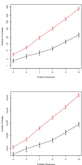
Figure 1 (top) reports, for each problem dimension, the average number of nodes found in the local optima net-works. The search difficulty of these landscape is ex-pected to increase with the number of local optima, and
1there, though, random values are uniformly distributed in[0, 99] 2with this choice for units position distribution, real-like instances
this value grows exponentially with the problem dimen-sion. Real-like instances, though, result in much smaller networks (small number of vertexes); the size difference between the two classes of QAP also grows almost expo-nentially with the problem dimension.
Figure 1 (bottom) shows a similar growth for the aver-age number of edges. Indeed, the graphs are almost fully connected, i.e. the number of oriented edges is close to the squared number of nodes.
3.2.2 Basins of attraction
Figure 2 depicts the average size of the basin of attraction of the global optimum divided by the size of the search space. This value decreases exponentially with the prob-lem dimension for both considered classes of QAP in-stances. The real-like instances present larger global opti-mum basins, which can be explained by their smaller lo-cal optima networks (this suggested explanation is further elaborated below). The relative size of the global opti-mum basin gives the probability of finding the best solu-tion with a hill-climbing algorithm from a random starting point. The exponential decrease confirms that the higher the problem dimension, the lower the probability for a stochastic search algorithm to locate the basin of attrac-tion of the global minimum. Considering the separaattrac-tion between the curves in fig. 2, it looks surprisingly easier to solve exactly a real-like instance rather than a uniform one.
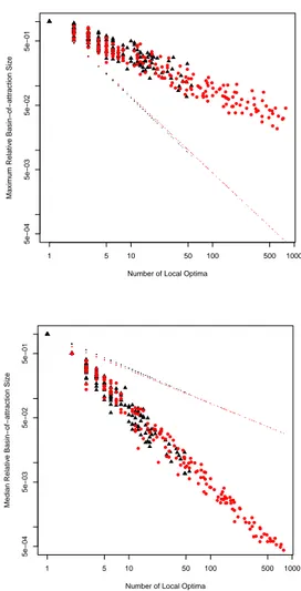
The distribution of basins sizes is very asymmetrical, thus the median and maximum sizes are used as represen-tatives3. These statistics are divided by the search space
size and plotted against the number of local optima (fig-ure 3) in order to convey a view independent of problem dimension and LON cardinality.
The median and maximum basin sizes follow a power-law relationship with the number of local optima. The difference between the two values tends to diverge expo-nentially with the LON size. This suggests that the land-scapes are characterized by many small basins and few larger ones. The correlation coefficients of the real-like and uniform instances are similar. Both instance classes seem to have the same size distribution with respect to the local optima network cardinality. This fact, coupled with
3the average basins size, equal to the number of possible
configura-tion in the search space divided by the number of local optima, is not informative
the different number of local optima but a similar distri-bution of basin sizes, can explain how real-like instances have larger global optimum basin compared to uniform instances of the same problem dimension.
Figure 4 plots the correlation coefficients between the logarithm of local optima basin sizes and their fitness value. There is a strong positive correlation. In other words, generally the better the fitness value of an opti-mum, the wider its basin of attraction. It is worth notic-ing, however, that the relative size of the global optimum (to the search space dimension), decreases exponentially as the problem size increases (see fig.2). Real-like and uniform instances show a similar behavior but the former present higher variability and slightly lower correlation figures.
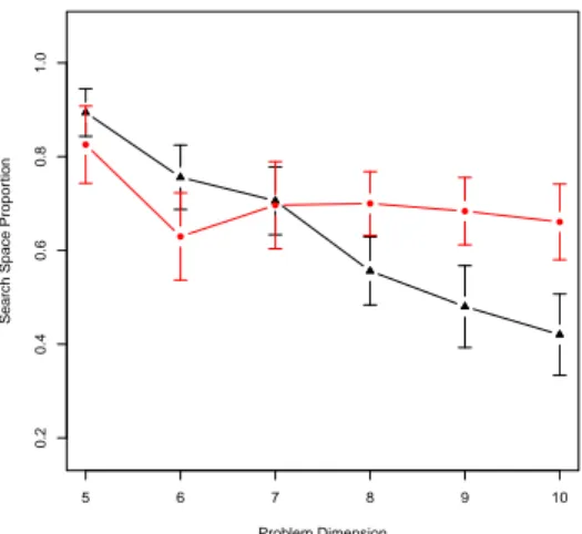
From what has been studied, real-like instances are eas-ier to solve exactly using heuristic search. However, Merz and Freisleben [12] have shown that the quality of local optima decreases when there are few off-diagonal zeros in the flow matrix: the cost contributions to the fitness value in eq.1 are in that case more interdependent, as there was a higher epistasis. Thus it should be easier to find a sub-optimal solution for a uniform instance than for a real-like one. To confirm this result in another way, figure 5 shows the proportion of solutions from whose a best im-provement hill-climbing conducts to a local optima within a5% value from the global optimum cost. As problem size grows, sub-optimal solutions are distinctively easier to reach in the uniform case, i.e. uniform instances are easier to be solved approximatively. This also agrees with the fact that for large enough instances, the cost ratio be-tween the best and the worst solution has been proved to converge to one in the random uniform case [13].
3.2.3 Transition probabilities
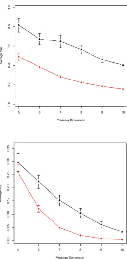
Figure 6 (top) reports for each problem dimension the av-erage weightwii of self-loop edges. These values
rep-resent the one-step probability of remaining in the same basin after a random move. The higher values observed for real-like instances are related to their fewer optima but bigger basins of attraction. However, the trend is gener-ally decreasing with the problem dimension. This is an-other confirmation that basins are shrinking with respect to their relative size.
wij of the outgoing links from each vertexi, as figure 6
(bottom) reports. Since j 6= i, these weights represent the probability of reaching the basin of attraction of one of the neighboring local optima. These probabilities de-crease with the problem dimension. The difference be-tween the two classes of QAP could be explained here by their different LON size.
A clear difference in magnitude betweenwii andwij
can be observed. This means that, after a move operation, it is more likely to remain in the same basin than to reach another basin. Moreover, the decreasing trend with the problem dimension is stronger forwijthan forwii,
espe-cially for the uniform QAP (whose LON grows faster with the problem dimension). Therefore, even for these small instances, the probability of reaching a particular neigh-boring basin becomes rapidly smaller than the probability of staying in the same basin, by an order of magnitude.
3.2.4 Weighted connectivity
In weighted networks, the degree of nodes is extended by defining the node strengthsias the sum of all the weights
wij of the links attached to it. This value gathers
infor-mation from both the connectivity of a node and the im-portance of its links [14]. In our definition, the out-going weights always sum up to 1, so the out-going strength is just1 − wii. Therefore, a study ofsi associated to the
in-coming links would be more informative.
Figure 7 reports the average vertex strength for connec-tions entering the considered basin. The increase with the problem dimension and the separation between the two QAP classes should come as no surprise since strength is related to vertex degree (which is higher for bigger LONs, given that they are almost complete). In particular, if the distribution of weights were independent of topology, the strength would be simply equal to the vertex degree multi-plied by the mean edge weight. These expected curves are plotted in dotted form and, although there is some clear correlation, the actual strengths are distinctively lower.
Figure 8 shows the aggregated average ofsi with
re-spect to the vertex in-degree ki for all the instances of
dimension 10. As the figure suggests, a fit with the law s = w ∗ k does not hold. Given the high connectivity of these LONs, the degree values are all close to the max-imum possible for each network. Thus, the strength of vertexes must grow much faster than their degree in order
to give the averages seen in fig. 7. It can be observed that, for uniform QAP instances, the scatter plot of fig. 8 is constituted by several curves that are almost vertical even in log-log scale. Real-like instances, on the contrary, have so smaller and densely connected LONs that an analogue behavior can not be spotted. However, for both instance classes, fig. 8 clearly suggests that the strength is far from being simply proportional to the vertex degree. Therefore, we have a confirmation that the distribution of weights, as we have defined them, strongly depends on the network topology.
Figure 9 reports the correlation coefficients between the in-coming strength of a vertex and the fitness value of its local optimum. The correlation is positive and strong, which suggests that basins with high fitness generally have more heavy weighted connectivity. Our explanation to this observation is the following: with our definition of transition probabilities, basin sizes have an influence on weight values. Also, there is a high correlation between the logarithmic size of a basin and its fitness value (see fig. 4).The same considerations made there still hold here, with the difference that the link between strength and fit-ness seems less tight as the size of problem grows. This could add to the search difficulty.
3.3
Advanced network features
3.3.1 Transitivity
Transitivity measures the probability that the adjacent ver-texes of a vertex are connected [15], this feature is mea-sured with the so called clustering coefficient. The tra-ditional definition of this coefficient does not consider weights, thus, it has been extended in several ways to a
weighted clustering coefficient [14]. Since our studied LONs from the QAP instances are close to be complete graphs, we selected the simplest definition. All the in-stances were found to have a transitivity value higher than 0.90: real-like instances have a value above 0.99, whereas uniform instances present a slight decrease with respect to the size of the problem. We also observed that this mea-sure has a lower variability when compared to the other networks statistics. Thus, a very high clustering coeffi-cient appears to be an instance independent characteristic of QAP with the given definition of LON.
3.3.2 Disparity
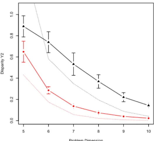
Another network statistic, which measures how heteroge-neous are the contributions of the edges of a nodei to its strengthsi, is disparity [14]. Disparity could be defined
asY2(i) = Pj6=i( wij
si )
2and could be averaged over the
nodes with the same degreek. If all the weights wij are
close tosi/ki, thenY2(i) ≈ 1/kifor nodes of degreeki.
Figure 10 reports the simple mean of disparity coeffi-cient averaged on all instances of both classes with respect to problem dimension. The decreasing trend could render the fact that as the size of the problem rises, the out-going transition to different optima neighbors tend to become equally probable and the search becomes more random. That could be more evident for uniform instances whose LONs have higher cardinality. Real-like instances, actu-ally, appear to maintain a disparity value less close to the random curve of1/k.
In figure 11 the aggregate average ofY2(i) to kiis
plot-ted on double logarithmic scale. Here just instances of problem dimension 10 have been considered. Disparity as a function of the node out-degree seems to follow a power-law, but as seen in fig. 10 that law is not the simple 1/ki. Thus it can be observed that, even if the weights
wij are not all equal tosi/ki, it remains difficult to spot
an out-going connection whose probability dominates the others, except for really small problem instances4. Ac-cording to the disparity measure, the real-like instances are not more difficult than uniform instances. No direc-tion is pointed out by the weights distribudirec-tion, and it must be considered to design efficient heuristics for QAP.
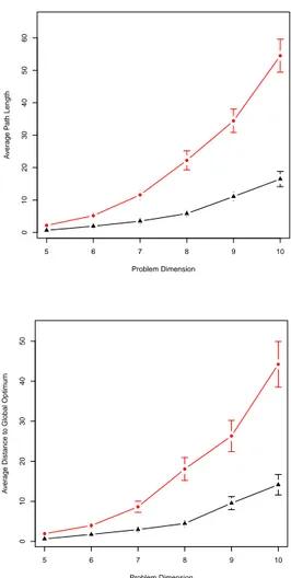
3.3.3 Shortest paths
A distance between two neighboring local optimai and j can be computed as the inverse of the transition probabil-ity between them: 1/wij. This value can be interpreted
as the expected number of random moves needed to hop from basin i to basin f j. The average path length can then be calculated as the average of all the shortest paths between any two nodes (see figure 12 (top)).
Figure 12 (bottom), reports a related measure, namely the mean shortest distance from each node to the global optimum. This metric can be more interesting from the
4the one connection who really could rise disparity figures is the
self-loop, but that has to be excluded by definition from the calculation of Y2
point of view of a stochastic local search heuristic trying to solve the considered QAP instance. The clear trend is that this path, as any other, increases with the prob-lem size. Values are noticeable higher for the uniform instances, which have a larger number of local optima than the real-like instance for the same problem dimen-sion. The figures confirm that the search difficulty in-creases with the domain size and the ruggedness of the fitness landscape (i.e. the number of local optima).
4
Discussion and Conclusions
We have used the recently proposed Local Optima
Net-work (LON)model to analyze the landscape of the well-known Quadratic Assignment Problem (QAP). Two types of instances: uniform and real-like, were analyzed and compared. The comparative analysis, show features clearly distinguishing these two types of QAP instances. Apart from a clear confirmation that the search difficulty increases with the problem dimension, the results provide new confirming evidence explaining why the real-like stances are easier to solve exactly, while the uniform in-stances are easier to solve approximately using stochastic local search.
A comparison of the LON of QAP against those of the previously studiedN K landscapes [1, 2, 3], suggests that the distributions of basin sizes, including the global opti-mum basin, are similar for comparable instances of QAP andN K. The main difference lies in the connectivity: whereas the LON is nearly a complete graph for QAP, this is not the case for N K landscapes. This could be due to the larger neighborhood size in the permutation space, as compared with the binary space. With the cur-rent move operations, the probability of exploring another basin from a solution by a random move is higher for com-parable QAP andN K instances. This suggests that the most efficient local searcher (based on those moves), for each problem should be different: the tradeoff between exploration and exploitation should not be the same. The aforementioned comparison could also permit to better explain the parallel between some flow matrix character-istics of QAP and the epistasis value ofN K. In particu-lar, the influence of flow dominance, a metric often used to characterize QAP instances, has not been directly ad-dressed in this paper, and it surely deserves more attention
and space. There may be also a connection between the present work and the concept of elementary landscapes, as QAP spaces or parts thereof might be spectrally de-composable in such way [9].
There are several directions for future work. Our cur-rent definition of transition probabilities, although very informative, may produce highly connected networks, which are not easy to study. Therefore, we are currently considering alternative definitions based on threshold val-ues for the connectivity. A high variability (across in-stances) on some metrics was observed, especially for the real-like class. Therefore, further analysis may need to be focused on particular instances, instead of on a statistical aggregation of a set of instances of (arguably) the same class. Moreover, our current methodology is only appli-cable to small problem instances. Good sampling tech-niques are required in order to extend the applicability of the model. The consideration of a permutation space in this article, opens up the possibility of analyzing other permutation based problems such as the traveling sales-man and the permutation flow shop problems. In addi-tion, it would be useful to compare results based on LON representation with those arising from theoretical analy-ses such as [16].
Finally, although the local optima network model is still under development, we argue that it offers an alternative view of combinatorial fitness landscapes, which can po-tentially contribute to both our understanding of problem difficulty, and the design of effective heuristic search al-gorithms, including evolutionary algorithms.
Acknowledgment
Fabio Daolio and Marco Tomassini gratefully acknowl-edge the Swiss National Science Foundation for financial support under grant number 200021-124578.
References
[1] G. Ochoa, M. Tomassini, S. V´erel, and C. Darabos, “A study of NK landscapes’ basins and local optima networks,” in Genetic and Evolutionary
Computa-tion Conference, GECCO 2008. ACM, 2008, pp. 555–562.
[2] S. Verel, G. Ochoa, and M. Tomassini, “The connec-tivity of NK landscapes’ basins: a network analysis,” in Artificial Life XI: Proceedings of the Eleventh
In-ternational Conference on the Simulation and Syn-thesis of Living Systems. MIT Press, Cambridge, MA, 2008, pp. 648–655.
[3] M. Tomassini, S. V´erel, and G. Ochoa, “Complex-network analysis of combinatorial spaces: The NK landscape case,” Phys. Rev. E, vol. 78, no. 6, p. 066114, 2008.
[4] J. P. K. Doye, “The network topology of a potential energy landscape: a static scale-free network,” Phys.
Rev. Lett., vol. 88, p. 238701, 2002.
[5] J. P. K. Doye and C. P. Massen, “Characteriz-ing the network topology of the energy landscapes of atomic clusters,” J. Chem. Phys., vol. 122, p. 084105, 2005.
[6] S. A. Kauffman, The Origins of Order. New York: Oxford University Press, 1993.
[7] T. C. Koopmans and M. Beckmann, “Assignment problems and the location of economic activities,”
Econometrica, vol. 25, no. 1, pp. 53–76, 1957.
[8] S. Sahni and T. Gonzalez, “P-complete approxima-tion problems,” Journal of the ACM (JACM), vol. 23, no. 3, pp. 555–565, 1976.
[9] P. F. Stadler, “Fitness landscapes,” in Biological
Evolution and Statistical Physics, ser. Lecture Notes Physics, M. L¨assig and Valleriani, Eds., vol. 585. Heidelberg: Springer-Verlag, 2002, pp. 187–207.
[10] J. Knowles and D. Corne, “Instance generators and test suites for the multiobjective quadratic assign-ment problem,” in Evolutionary Multi-Criterion
Op-timization, Second International Conference, EMO 2003, Faro, Portugal, April 2003, Proceedings, ser. LNCS, no. 2632. Springer, 2003, pp. 295–310.
[11] ´Eric D. Taillard, “Comparison of iterative searches for the quadratic assignment problem,” Location
[12] P. Merz and B. Freisleben, “Fitness landscape analy-sis and memetic algorithms for the quadratic assign-ment problem,” IEEE Transactions on Evolutionary
Computation, vol. 4, no. 4, pp. 337–352, 2000. [13] P. Krokhmal and P. Pardalos, “Random assignment
problems,” European Journal of Operational
Re-search, vol. 194, no. 1, pp. 1–17, 2009.
[14] M. Barth´elemy, A. Barrat, R. Pastor-Satorras, and A. Vespignani, “Characterization and modeling of weighted networks,” Physica A, vol. 346, pp. 34–43, 2005.
[15] S. Wasserman and K. Faust, Social network
analy-sis: Methods and applications. Cambridge Univer-sity Press, 1994.
[16] T. Chen, J. He, G. Chen, and X. Yao, “Choosing selection pressure for wide-gap problems,”
Theoret-ical Computer Science, vol. 411, no. 6, pp. 926 – 934, 2010. 5 6 7 8 9 10 1 2 5 10 20 50 100 200 500 Problem Dimension Number of V er te x es ● ● ● ● ● ● 5 6 7 8 9 10 1e+01 1e+02 1e+03 1e+04 1e+05 Problem Dimension Number of Edges ● ● ● ● ● ●
Figure 1: Average number of nodes (top) and edges (bot-tom) on log-lin scale. Triangular points correspond to real-like problems, rounded points to uniform ones; bars show 95% Wald C.I. on the means; for each problem dimension, averages from 30 independent and randomly generated instances are shown.
5 6 7 8 9 10 0.05 0.10 0.20 0.50 1.00 Problem Dimension Basins−of−attr action Relativ e Siz e of Global Optim um ● ● ● ● ● ●
Figure 2: Average relative size of the global optimum basin-of-attraction on log-lin scale. Triangular points cor-respond to real-like problems, rounded points to uniform ones; bars show 95% Wald C.I. on the means; for each problem dimension, averages from 30 independent and randomly generated instances are shown.
1 5 10 50 100 500 1000
5e−04
5e−03
5e−02
5e−01
Number of Local Optima
Maxim um Relativ e Basin−of−attr action Siz e ● ● ● ● ● ● ● ● ● ● ● ● ● ● ● ● ● ● ● ● ● ● ● ● ● ● ● ● ● ● ● ● ● ● ● ● ● ● ● ● ● ● ● ● ● ● ● ● ● ● ● ● ● ● ● ● ● ● ● ● ● ● ● ● ● ● ● ● ● ● ● ● ● ● ● ● ● ● ● ● ● ● ● ● ● ● ● ● ● ● ● ● ● ● ● ● ● ● ● ● ● ● ● ● ● ● ● ● ● ● ● ● ● ● ● ● ● ● ● ● ● ● ● ● ● ● ● ● ● ● ● ● ● ●● ● ● ● ● ● ● ● ● ● ● ● ● ● ● ● ● ● ● ● ● ● ● ● ● ● ● ● ● ● ● ● ● ● ● ● ● ● ● ● ● ● ● ● ● ● 1 5 10 50 100 500 1000 5e−04 5e−03 5e−02 5e−01
Number of Local Optima
Median Relativ e Basin−of−attr action Siz e ● ● ● ● ● ● ● ● ● ● ● ● ● ● ● ● ● ● ● ● ● ● ● ● ● ● ● ● ● ● ● ● ● ● ● ● ● ● ● ● ● ● ● ● ● ● ● ● ● ● ● ● ● ● ● ● ● ● ● ● ● ● ● ● ● ● ● ● ● ● ● ● ● ● ● ● ● ● ● ● ● ● ● ● ● ● ● ● ● ● ● ● ● ● ● ● ● ● ● ● ● ● ● ● ● ● ● ● ● ● ● ● ● ● ● ● ● ● ● ● ● ● ● ● ● ● ●● ● ● ● ● ● ●● ● ● ● ● ● ● ● ● ● ● ● ● ● ● ● ● ● ● ● ● ● ● ● ● ● ● ● ● ● ● ● ● ● ● ● ● ● ● ● ● ● ● ● ● ●
Figure 3: Relative size of the largest (top) and of the me-dian (bottom) basin of attraction vs number of nodes. Tri-angular points correspond to real-like instances, rounded points to uniform ones. Each figure reports in dotted form the regression lines of the other.
5 6 7 8 9 10 0.0 0.2 0.4 0.6 0.8 1.0 Problem Dimension Fit.V
alue vs log10 Bas
.Siz e Correlation Coefficient ● ● ● ● ● ●
Figure 4: Average Fit.Value vs Bas.Size Correlation Co-efficient. Triangular points correspond to real-like prob-lems, rounded points to uniform ones; bars show 95% Wald C.I. on the means; for each problem dimension, av-erages from 30 independent and randomly generated in-stances are shown.
5 6 7 8 9 10 0.2 0.4 0.6 0.8 1.0 Problem Dimension
Search Space Propor
tion ● ● ● ● ● ●
Figure 5: Proportion of search space whose solutions climb to a fitness value within 5% from the global best value. Triangular points correspond to real-like problems, rounded points to uniform ones; for each problem dimen-sion, averages from 30 independent and randomly gener-ated instances are shown.
5 6 7 8 9 10 0.0 0.2 0.4 0.6 0.8 1.0 Problem Dimension A v er age Wii ● ● ● ● ● ● 5 6 7 8 9 10 0.00 0.05 0.10 0.15 0.20 0.25 0.30 0.35 Problem Dimension A v er age Wij ● ● ● ● ● ●
Figure 6: Average weights wii for self-loop (top) and
wij for out-going links (bottom). Triangular points
cor-respond to real-like instances, rounded points to uniform ones; bars show 95% Wald C.I. on the means; for each problem dimension, averages from 30 independent and randomly generated instances are shown.
5 6 7 8 9 10 0.0 0.2 0.4 0.6 0.8 1.0 Problem Dimension A v er age in−Si ● ● ● ● ● ●
Figure 7: Average vertexes in-coming strength. Trian-gular points correspond to real-like problems, rounded points to uniform ones; bars show 95% Wald C.I. on the means; dotted lines report the mean in-coming degree multiplied by the mean edge weight; for each problem dimension, averages from 30 independent and randomly generated instances are shown.
●● ● ● ● ●● ● ● ● ● ● ● ● ● ● ●● ● ● ● ● ● ● ● ● ● ● ● ● ● ● ● ● ● ● ● ● ● ●●●● ● ● ● ● ● ● ● ● ● ●● ● ● ● ● ● ● ● ● ● ● ● ● ● ● ● ● ● ● ● ● ● ● ● ● ● ● ● ● ● ● ●● ● ● ● ● ● ● ● ● ● ●● ● ● ● ● ● ● ● ● ● ● ● ● ● ● ● ● ● ● ●● ● ● ● ● ●●● ● ● ● ● ● ● ● ● ● ● ● ● ●●●● ● ● ● ● ● ● ● ● ● ● ● ●●● ● ● ● ● ● ●● ● ● ● ● ● ● ● ● ● ● ● ● ● ● ● ● ● ● ● ● ● ● ● ●● ● ● ● ● ● ● ● ● ● ● ● ● ● ● ● ● ● ● ● ● ● ● ● ● ● ● ●●● ● ● ● ● ● ● ● ● ● ● ● ● ● ● ● ● ● ● ● ● ● ● ● ● ● ● ● ●● ● ● ● ● ● ● ● ● ● ●●● ● ● ● ● ● ● ● ● ●● ● ● ● ● ● ● ● ● ● ● ● ● ● ● ● ● ● ● ● ● ● ● ●●● ● ● ● ● ● ● ● ● ● ●● ● ● ● ● ● ● ● ● ● ● ● ●● ● ● ● ● ● ● ● ● ● ● ● ● ● ● ● ● ● ● ● ● ● ● ● ● ● ● ● ● ● ● ● ● ● ● ● ● ● ● ● ● ● ● ● ● ● ● ● ● ● ● ● ● ●● ● ● ● ● ● ● ● ● ● ● ● ● ● ●●● ● ● ● ● ● ● ● ● ● ● ● ● ● ● ● ● ● ● ● ● ● ● ● ● ● ● ● ● ● ● ● ● ● ● ● ● ● ● ● ● ● ● ● ● ● ● ● ● ● ● ● ● ● ● ● ● ● ● ● ● ● ●● ● ● ● ● ● ● ● ● ● ● ● ● ● ● ● ● ●●●●● ● ● ● ● ● ● ● ● ● ● ● ● ● ●● ● ● ● ● ● ● ● ● ● ● ● ● ● ● ● ● ●●● ● ● ● ● ● ● ● ● ● ● ● ● ● ● ● ● ● ● ● ● ● ● ● ● ● ● ● ● ● ● ● ● ● ● ● ● ● ● ● ● ● ● ● ● ● ● ● ● ● ● ● ● ● ● ● ●●●●● ● ● ● ● ● ● ● ● ● ● ● ● ● ● ● ● ●●● ● ● ● ● ● ● ● ● ● ● ● ● ● ● ● ● ● ● ●●● ● ● ● ● ● ● ● ● ● ● ● ● ● ● ● ● ● ● ● ● ● ● ● ● ● ● ● ● ● ● ● ● ● ● ● ● ● ● ● ● ● ● ●●●●●●●●●●●●●● ● ● ● ● ● ● ● ● ●● ● ● ● ● ● ● ● ● ● ● ● ● ● ● ● 1 5 10 50 100 500 1000 1e−03 1e−02 1e−01 1e+00 1e+01 In−Degree In−Strength
Figure 8: Aggregated average of strength to vertex in-degree on log-log scale. Triangular points correspond to real-like problems, rounded points to uniform ones; all 30 independent and randomly generated instances of prob-lem dimension 10 are shown. Dotted lines report the s = w ∗ k relation. 5 6 7 8 9 10 0.2 0.4 0.6 0.8 1.0 Problem Dimension Fit.V
alue vs In−Strength Correlation Coefficient
●
● ● ●
● ●
Figure 9: Average Fit.Value vs In-Strength Correlation Coefficient. Triangular points correspond to real-like problems, rounded points to uniform ones; bars show 95% Wald C.I. on the means; for each problem dimension, av-erages from 30 independent and randomly generated in-stances are shown.
5 6 7 8 9 10 0.0 0.2 0.4 0.6 0.8 1.0 Problem Dimension Dispar ity Y2 ● ● ● ● ● ●
Figure 10: Average disparity coefficient. Triangular points correspond to real-like instances, rounded points to uniform ones; bars show 95% Wald C.I. on the means; for each problem dimension, averages from 30 independent and randomly generated instances are shown.
● ● ●●●● ● ● ●●● ● ● ● ● ● ● ● ● ● ● ● ●● ● ● ● ● ● ● ●● ● ● ● ● ● ● ● ● ● ● ● ● ● ● ● ● ● ● ● ●● ● ● ● ●●●● ● ●●●●● ● ● ● ● ● ● ● ● ● ● ● ●● ● ● ● ● ●● ● ● ● ● ● ● ● ● ● ● ●● ● ● ● ● ● ● ● ● ● ● ● ●●●●●● ●●●●●●●● ● ● ● ● ● ● ●●● ● ● ● ● ● ●●●●● ● ● ● ● ● ● ● ● ● ● ●●● ● ● ● ● ● ●●●●●●●●●●●●●●● ● ● ●●●●● ● ● ● ● ●●●●● ● ● ● ● ●●●● ● ● ● ● ● ● ●●●●●●●● ● ●●●●●● ● ● ● ● ●●●●●●●●●●●●● ● ● ● ● ● ● ● ● ● ●●●● ● ● ● ● ● ● ● ●●●●●●●●●●●●● ● ● ● ● ● ● ● ● ● ● ●●●●●●●●●●●●●●●●●●●●●●●●●●●●●●●●●●●● ● ● ● ● ● ● ● ● ● ● ● ● ● ● ● ● ● ● ● ● ● ● ● ● ● ● ● ● ● ●●●●●●●●●●●●●●●●● ● ● ● ● ● ● ● ● ● ● ● ● ●●●●●●●●●● ● ● ● ● ● ● ●●●●● ● ● ● ● ● ● ● ● ● ● ●● ● ● ● ● ● ● ● ● ● ● ● ● ● ● ● ● ● ● ● ● ● ● ● ● ● ● ● ● ● ● ● ●●●●●●●● ● ● ● ● ● ● ● ● ● ● ●●● ● ● ● ● ● ● ● ● ● ● ● ● ● ● ● ●● ● ● ● ● ● ● ● ● ● ● ● ● ● ● ● ● ●●●●● ● ● ● ● ● ● ● ● ● ● ● ● ● ● ● ● ● ● ● ● ● ● ● ● ● ● ● ● ● ● ● ● ● ● ●●●●●●● ● ● ● ● ● ● ● ● ● ● ● ● ●●● ● ● ● ● ● ● ● ● ● ● ● ● ● ● ● ● ● ● ●● ● ● ● ● ● ● ● ● ● ● ● ● ● ● ● ● ● ● ● ● ● ● ● ● ● ● ● ● ● ● ● ● ● ● ● ● ● ● ● ● ● ● ●●● ● ● ● ● ● ● ● ● ● ● ● ● ● ● ● ● ● ● ● ● ●● ● ● ● ● ● ● ● ● ● ● ● ● ● ● ● ● ● ● ● ● ● ●● ● ● ● ● ● ● ● ● ● ● ● ● ● ● ● ● ● ● ● ● ● ● 1 5 10 50 100 500 1000 0.001 0.002 0.005 0.010 0.020 0.050 0.100 0.200 Out−Degree Dispar ity
Figure 11: Aggregated average of disparity coefficient to vertex out-degree. Triangular points correspond to real-like instances, rounded points to uniform ones; all 30 in-dependent and randomly generated instances for problem size 10 are shown. Dotted lines report the inverse of the out-going degree. 5 6 7 8 9 10 0 10 20 30 40 50 60 Problem Dimension A v er age P ath Length ● ● ● ● ● ● 5 6 7 8 9 10 0 10 20 30 40 50 Problem Dimension A v er
age Distance to Global Optim
um ● ● ● ● ● ●
Figure 12: Average path length (top) average shortest path to global optimum (bottom). Triangular points cor-respond to real-like problems, rounded points to uniform ones; bars show 95% Wald C.I. on the means; for each problem dimension, averages from 30 independent and randomly generated instances are shown.