HAL Id: hal-00317811
https://hal.archives-ouvertes.fr/hal-00317811
Submitted on 27 Jul 2005
HAL is a multi-disciplinary open access
archive for the deposit and dissemination of
sci-entific research documents, whether they are
pub-lished or not. The documents may come from
teaching and research institutions in France or
abroad, or from public or private research centers.
L’archive ouverte pluridisciplinaire HAL, est
destinée au dépôt et à la diffusion de documents
scientifiques de niveau recherche, publiés ou non,
émanant des établissements d’enseignement et de
recherche français ou étrangers, des laboratoires
publics ou privés.
The red-sky enigma over Svalbard in December 2002
F. Sigernes, N. Lloyd, D. A. Lorentzen, R. Neuber, U.-P. Hoppe, D.
Degenstein, N. Shumilov, J. Moen, Y. Gjessing, O. Havnes, et al.
To cite this version:
F. Sigernes, N. Lloyd, D. A. Lorentzen, R. Neuber, U.-P. Hoppe, et al.. The red-sky enigma over
Svalbard in December 2002. Annales Geophysicae, European Geosciences Union, 2005, 23 (5),
pp.1593-1602. �hal-00317811�
Annales Geophysicae, 23, 1593–1602, 2005 SRef-ID: 1432-0576/ag/2005-23-1593 © European Geosciences Union 2005
Annales
Geophysicae
The red-sky enigma over Svalbard in December 2002
F. Sigernes1, N. Lloyd2, D. A. Lorentzen1, R. Neuber3, U.-P. Hoppe4, D. Degenstein2, N. Shumilov1,5,*, J. Moen1,6, Y. Gjessing1,7, O. Havnes1,5, A. Skartveit7, E. Raustein7,*, J. B. Ørbæk8, and C. S. Deehr9
1The University Centre in Svalbard (UNIS), N-9171 Longyearbyen, Norway
2ISAS, University of Saskatchewan, Saskatoon, Canada
3Alfred Wegener Institute for Polar and Marine Research, Potsdam, Germany
4Norwegian Defence Research Establishment, Kjeller, Norway
5The Auroral Observatory, University of Tromsø, Norway
6Department of Physics, University of Oslo, Oslo, Norway
7Geophysical Institute, University of Bergen, Bergen, Norway
8The Norwegian Polar Institute, Longyearbyen, Svalbard, Norway
9Geophysical Institute, University of Alaska, Fairbanks, USA
*Deceased
Received: 31 August 2004 – Revised: 13 January 2005 – Accepted: 17 January 2005 – Published: 27 July 2005 Part of Special Issue “Atmospheric studies by optical methods”
Abstract. On 6 December 2002, during winter
dark-ness, an extraordinary event occurred in the sky, as viewed
from Longyearbyen (78◦N, 15◦E), Svalbard, Norway. At
07:30 UT the southeast sky was surprisingly lit up in a deep red colour. The light increased in intensity and spread out across the sky, and at 10:00 UT the illumination was
ob-served to reach the zenith. The event died out at about
12:30 UT. Spectral measurements from the Auroral Station in Adventdalen confirm that the light was scattered sunlight. Even though the Sun was between 11.8 and 14.6 deg be-low the horizon during the event, the measured intensities of scattered light on the southern horizon from the scanning photometers coincided with the rise and setting of the Sun. Calculations of actual heights, including refraction and at-mospheric screening, indicate that the event most likely was scattered solar light from a target below the horizon. This is also confirmed by the OSIRIS instrument on board the Odin satellite. The deduced height profile indicates that the scattering target is located 18–23 km up in the stratosphere
at a latitude close to 73–75◦N, southeast of Longyearbyen.
The temperatures in this region were found to be low enough for Polar Stratospheric Clouds (PSC) to be formed. The tar-get was also identified as PSC by the LIDAR systems at the
Koldewey Station in Ny- ˚Alesund (79◦N, 12◦E). The event
was most likely caused by solar illuminated type II Polar Stratospheric Clouds that scattered light towards Svalbard. Two types of scenarios are presented to explain how light is scattered.
Correspondence to: F. Sigernes
Keywords. Atmospheric composition and structure (Trans-missions and scattering of radiation; Middle atmosphere-composition and chemistry; Instruments and techniques) – History of geophysics (Atmospheric Sciences; The red-sky phenomena)
1 Introduction
The Auroral Station in Adventdalen, Svalbard (78◦N,
15◦E), close to the town of Longyearbyen (LYR), is a
multi-instrument platform for studies of dayside aurora and other high latitude optical phenomena. It is more or less com-pletely dark during the day for more than 2 months in the middle of the winter. Near winter solstice the Sun is at least 10 deg below the horizon at noon. Hence, it should be almost completely dark in the daytime at Longyearbyen during the months of December and January. But, to our surprise, on 6 December 2002, the southeast sky turned deep red from about 07:30 to 12:30 UT. The scattered light from the event turned the polar night into day. In fact, the light was so in-tense that the whole valley of Adventdalen was visible to the human eye − an effect that is usually not seen at this time of the year except in the light of the full moon.
The whole event caused great public attention. Questions about its origin were very soon directed to the Auroral Sta-tion. In the early stages of the event, it was even speculated that a nuclear bomb explosion must have taken place. The Governor of Svalbard was on the alert and the local news-paper made headlines in Norway with the article titled “A
1594 F. Sigernes et al.: Atmospheric studies by optical methods
18 Figure 1. Photograph of the event taken from the Auroral Station in Adventdalen, Svalbard, Norway, at 08:42:41 UT 06.12.2002. The exposure time is 20 second at F/2.8 using a 14 mm lens with a Fujifilm S2Pro camera body. The sensitivity is ISO 200.
Fig. 1. Photograph of the event taken from the Auroral Station in Adventdalen, Svalbard, Norway, at 08:42:41 UT on 6 December 2002. The exposure time is 20 s at F/2.8, using a 14–mm lens with a Fujifilm S2Pro camera body. The sensitivity is ISO 200.
mysterious phenomena” (Pedersen, 2002). It is safe to say that during the morning hours of 6 December 2002, we were first scared by the event. Later on, this feeling turned into curiosity.
At the time of the event The Auroral Station in Advent-dalen was fully operative with all its instruments, which were set up to study optical signatures of the dayside aurora. A
re-mote controlled spectrometer located in Ny- ˚Alesund (NYA;
79◦N, 12◦E) was also operative. Ny- ˚Alesund is 118 km
north of Longyearbyen. Fortunately, data from the OSIRIS instrument on board the Odin satellite and data from the
LI-DARS at the Koldewey Station in Ny- ˚Alesund are also
avail-able. This study presents both the ground-based and the space-borne measurements of the event. Finally, a discussion is given on what might be the cause of the red-sky event.
2 Ground-based observations
The ground-based data set consists of photographs, photome-ter scans along the magnetic meridian, wavelength spectra obtained in the zenith from both Longyearbyen and
Ny-˚
Alesund, and multi-wavelength LIDAR height profiles from
the Koldewey Station in Ny- ˚Alesund.
2.1 Weather conditions
The sky on 6 December 2002 was partly cloudy over the station with normal wind conditions at ground level. The average wind speed from southeast was 7.2 m/s at the 10-m height level. There was, in other words, a light breeze blowing down the valley (Adventdalen) toward the sea (Is-fjorden). The pressure was high (1022 mbar), with a daily average temperature of +5.4 deg Celsius, which is close to 19 deg Celsius above the daily average temperature for this date measured from 1976 to 1989. In fact, the whole pe-riod from November to December was characterized as be-ing much warmer than the normal conditions. A strong heat
advection from the south led to the observed ground temper-atures close to +5 deg Celsius.
2.2 Image gallery
High resolution digital photographs of the event were ob-tained by using a Fujifilm FinePixS2Pro camera body with a wide-angle 14-mm focal length len. The original images are 4256×2848 pixels. Figure 1 shows an unprocessed image taken from the Auroral Station pointing towards the south-east, with the lights of Mine 7 and EISCAT close to the cen-tre of the image. The exposure time was 20 s at f/2.8. Note the deep red-coloured snow-covered ground, indicating that strong multiple scattering took place in the troposphere.
2.3 Meridian scanning photometers
The Meridian Scanning Photometer (MSP) has 5 channels, where each channel consists of a narrow bandpass filter mounted in a tilting frame. The tilting filter is in front of a 3” telescope with a cooled photomultplier (the detector). These tilting filter photometers are placed in front of a ro-tating mirror, which scans the sky from north to south along the geo-magnetic meridian. The instrument delivers inten-sity as a function of elevation angles in the meridian plane in 5 wavelength bands. The field of view is approximately one degree for each channel. The principal wavelengths used in
this study are the auroral 5577, 6300 and the 8446 ˚A
emis-sion lines of atomic oxygen. In addition, we use the auroral
4278 ˚A emission band of molecular nitrogen [N+21NG] and
the 4861 ˚A Doppler broadened profile of hydrogen [Hβ]. The
latter emission is normally produced by proton precipitation, producing hydrogen aurora. Each filter has a bandpass of
ap-proximately 5 ˚A. The background for each filter is obtained
by tilting the filters from peak transmission position at the line emission of interest to an angle that transmits the base wavelength representing the background emissions (BASE). The shift angle is chosen to change the peak wavelength at least 2 times the bandpass. Data is recorded over the merid-ian every 16 s (2×4-s-scan line peak; 2×4 s of BASE).
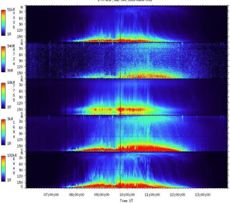
In Fig. 2 the background or BASE data is shown. The peak values are not used because they are contaminated by the above mentioned auroral emissions. The Near Infra Red (NIR) channel observed the strongest intensities. The inten-sities decreased with wavelength towards the blue. Note that the data is colour coded in Fig. 2 from black to red in units of Rayleighs, as given by the colour bars to the left. The colour red represents intensities at or above the given maxi-mum numbers. For example, a closer look at 10:00 UT
re-veals that the 8446 ˚A channel illumination rises quickly from
the horizon up to a maximum at about 168 deg, followed by a relatively slow decrease to the zenith (90 deg). The max-imum intensity is above 200 kR at 168 deg. For the other channels, the maximum intensities are 70, 15, 5 and 0.8 kR
for the 6300, 5577, 4861 and 4278 ˚A channels, respectively.
F. Sigernes et al.: Atmospheric studies by optical methods 1595
19 Figure 2. Meridian Scanning Photometer (MSP) data (BASE Only) from the Auroral Station in Adventdalen, Norway, 06:00 - 14:00 UT, 06.12.2002. The intensities are indicated as coloured bars to the left for each channel with centre wavelengths 6300, 4278, 5577, 4861 and 8446 Å, respectively. The intensities are in kilo Rayleighs [kR]. South is 180o in scan angle. Note that solar depression angles were 12.6°, 10.7°, and 11.8° at 08:30 UT, 10:30 UT and 12:30 UT, respectively.
Fig. 2. Meridian Scanning Photometer (MSP) data (BASE Only) from the Auroral Station in Adventdalen, Norway, 06:00–14:00 UT, 6 December 2002. The intensities are indicated as coloured bars to the left for each channel with centre wavelengths 6300, 4278, 5577, 4861 and 8446 ˚A, respectively. The intensities are in kilo Rayleighs [kR]. South is 180◦in scan angle. Note that solar depression angles were 12.6◦, 10.7◦, and 11.8◦ at 08:30 UT, 10:30 UT and 12:30 UT, respectively.
profiles, except for the green channel which has a stronger local maximum at 150 compared to the one at 168 deg.
2.4 Spectrometers
The Ebert-Fastie spectrometers used in this study were orig-inally designed by Fastie (1952a,b). Two instruments with 1 m focal length were operated from Longyearbyen (designa-tors Green LYR and Silver LYR), and one 1/2 m focal length instrument in Ny- ˚Alesund (designator Black Ny ˚A).
The principal components of the instruments are one large 1m focal length spherical mirror (1/2 m focal length for
Black Ny ˚A), one plane reflective diffraction grating and a
pair of curved slits. The recorded radiance from the sky is limited by the etendue; the product of the area of the en-trance slit and the field of view. Because the intensity of the source is usually low, the etendue is made as large as possi-ble. The image of the entrance slit is reflected by one part of the spherical mirror onto the grating. The second part of the mirror focuses the diffracted light from the grating onto the exit slit. When the grating turns, the image of the entrance slit is scanned across the exit slit. A collector lens transfers the output of the exit slit to the front of a photo multiplier tube. The tube is mounted in a Peltier cooled housing. Signals from the tube are amplified and discriminated before being sent to the computer counting card.
In Fig. 3, the green curves are time-averaged spectra be-fore the event, representing normal conditions with intensi-ties in R/ ˚A on the right hand axis. The red curves are the cor-responding spectra of our event with intensities in R/ ˚A on the left hand axis. First of all, the normal or background spec-tra show known familiar features. In panel (A) and (B), the
4861 ˚A [Hβ] and the 6563 ˚A [Hα] Doppler broadened
emis-sion lines of hydrogen appear. The source of the emisemis-sion profiles is proton precipitation, causing the dayside hydro-gen aurora. Also, throughout panel (B), (C) and (D) the airglow emission lines of hydroxyl OH(6,1), OH(8,3) and OH(6,2) are dominating the spectrum, especially in the NIR region of the spectrum. The emission lines at 6300 ˚A, 6364 ˚A
(Panel B) and 8446 ˚A (Panel D) are oxygen [OI] lines
pro-duced by electron precipitation. Other known auroral lines
are the 7320/30 ˚A doublet of oxygen [OII] (Panel C).
In addition, high resolution, ground-based, direct solar
spectra (Full Width at Half Maximum; FWHM=0.002 ˚A)
have been obtained from the BASS2000 tool provided by the Solar Survey homepage (http://mesola.obspm.fr/). In or-der to compare with the event (red curves), these spectra have been convolved with the instrumental functions corre-sponding to the bandpass of our instruments. Furthermore, the spectra are normalized to the intensities of our measure-ments. The scaling factors are shown in each panel. Com-parison of the resulting spectra (the yellow curves in Fig. 3)
1596 F. Sigernes et al.: Atmospheric studies by optical methods
20 Figure 3. Spectrometer data of the Dec. 6, 2002 event from the Auroral Station in Adventdalen (Panel A and D) and from the station in Ny-Ålesund (Panel B and C). Green curves are prior to the event, indicating the normal dark sky conditions. Red spectra are from the event itself. The yellow curves are a model spectrum of the sun. The intensities are in Rayleighs / Ångstrøm [R/Å] on both the left and right hand y-axis. The right hand axis represents normal conditions (green curve).
Fig. 3. Spectrometer data of the 6 December 2002 event from the Auroral Station in Adventdalen (Panel A and D) and from the sta-tion in Ny- ˚Alesund (Panel B and C). Green curves are prior to the event, indicating the normal dark sky conditions. Red spectra are from the event itself. The yellow curves are a model spectrum of the sun. The intensities are in Rayleighs/ ˚Angstrøm [R/ ˚A] on both the left and right hand y-axis. The right hand axis represents normal conditions (green curve).
21 Figure 4. ODIN / OSIRIS spectrum of the red-sky event at 12:47:43 UT, orbit # 9726, 06.12.2002. The target is located at position (74.4 oN, 49.9 oE). The altitude is 18.5 km.
Fig. 4. ODIN / OSIRIS spectrum of the red-sky event at 12:47:43 UT, orbit #9726,6 December 2002. The target is located at position (74.4◦N, 49.9◦E). The altitude is 18.5 km.
and the spectra measured by the spectrometer at the ground indicate that the source is the Sun. The main solar Fraun-hofer lines are all clearly identified to coincide with our spec-tra. Also the atmospheric water vapour absorption bands are identified in the NIR region.
From Fig 3 we also see that the scattered light of the event increased in intensity from the blue to the near infra-red. The
maximum intensity per wavelength unit varies from 70 R/ ˚A
for λgn the [4820–4920] ˚A range, 120 R/ ˚A for λ in the
[6280–6620] ˚A range, 375 R/ ˚A for λ in the [7250–7450] ˚A
Table 1. Estimated emission height profile at 800 nm from the OSIRIS instrument on the Odin satellite, orbit #9726, 6 December 2002. Altitude [km] Intensity (800 nm) [R/ ˚A] 26 40 23 90 18 320 15 250 10 250 6 230
range, and up to 1.5 kR/ ˚A for λ in the [8240–8570] ˚A range. Note that normal background values are in the range 5– 30 R/ ˚A.
3 Spaceborne observations
To our knowledge, the OSIRIS instrument on board the Odin satellite was the only space-borne instrument that where able to detect any signals from the 6 December 2002 event. The OSIRIS instrument measure spectral radiance height profiles over 280 to 800 nm from 5 to 70 km altitude at the Earth’s limb (Lloyd et al., 2005).
During orbit #9726, the Odin spacecraft measured en-hanced red spectra from 12:47:09 to 12:47:43 UT. The
spec-tra originated from an area that spanned from (72.67◦N,
53.47◦E) to (74.43◦N, 49.94◦E), which is slightly
south-east of Longyearbyen. Figure 4 shows a typical spectrum of the event as seen by the OSIRIS instrument. The spectra
show O2A-band absorption at 762 nm. The water vapour
ab-sorption feature is evident at ∼730 nm and the O2B-band at
∼690 nm is also evident. Note that the A-band absorption is
unreliable as the background signal that is subtracted (mostly dark current) does have significant A-band emissions.
The spatial resolution of OSIRIS is about 1 km in altitude by 30 km parallel to the Earth’s surface. The data shown in Table 1 are the radiances observed at 800 nm by OSIRIS in the limb at different tangent altitudes. Each observation cor-responds to the integral of the volume emission rate along the line of sight. Since OSIRIS is outside the Earth’s atmo-sphere, each line of sight observation must have contribu-tions from all altitudes above the tangent point.
When OSIRIS is looking at altitudes above a layer (26 km and above), there is no contribution from the layer to the in-tegrated line of sight signal. However when OSIRIS looks at tangent altitudes below or within the layer, then there is always some contribution to the observed radiance from the parts of the layer that are above the tangent point. The result is that you do not expect to see a sharp peak in intensity at the layer altitude but rather a steady decline in intensity as you look at altitudes below or within the layer.
F. Sigernes et al.: Atmospheric studies by optical methods 1597
22 Figure 5. Temperature height profiles from the European Centre for Medium Range Weather Forecast (ECMWF). The location is Andenes on Andøya, Norway (69.75N, 15.75E). Date is 06.12.2002. The profiles are colour coded according to a 6 hour sample period. Also shown are the height region where PSCs are formed together with the 5 ppmv H2O threshold
temperatures for NAT (dotted line), STS (dashed line) and ice (solid line).
Fig. 5. Temperature height profiles from the European Centre for Medium Range Weather Forecast (ECMWF). The location is An-denes on Andøya, Norway (69.75 N, 15.75 E). Date is 6 December 2002. The profiles are colour coded according to a 6 h sample pe-riod. Also shown are the height region where PSCs are formed to-gether with the 5 ppmv H2O threshold temperatures for NAT (dotted line), STS (dashed line) and ice (solid line).
Table 2. Different types of Polar Stratospheric Clouds (PSCs) ac-cording to composition (Voigt et al., 2000; Schreiner et al., 1999).
Type Composition
PSC Ia Solid Nitric acid Trihydrate; Nitric acid Dihydrate (NAT; NAD) particles ∼1 µm diameter.
PSC Ib Liquid ternary H2O / HNO3/ H2SO4solution (STS) droplets
PSC II Ice particles ∼10µm diameter
The main point to be taken from the OSIRIS radiance pro-file is that the sharp gradient between 18 and 23 km clearly locates the highest altitude of the layer within the strato-sphere. It definitely excludes mesospheric sources for the red-sky. Whether OSIRIS sees a narrow layer (less than 1 km) or a thick slab (many km thick) is not easily answered using the OSIRIS data. In principal it is possible to use the shape of the OSIRIS radiance profile to estimate the thick-ness of the layer but we have not done this as the data do not have sufficient spatial sampling or signal to noise to justify this analysis. Note that the brightness seen by OSIRIS is of
the same order of magnitude (a couple of hundred R/ ˚A) as
seen by the instrumentation at the Auroral station in Advent-dalen.
23 Figure 6. Northern hemisphere daily temperatures in the stratosphere from the European Centre for Medium Range Weather Forecast (ECMWF) at a potential temperature of 550K. Date is 06.12.2002. The profiles are colour coded according to temperature distribution. Fig. 6. Northern Hemisphere daily temperatures in the stratosphere from the European Centre for Medium Range Weather Forecast (ECMWF) at a potential temperature of 550K. Date is 6 Decem-ber 2002. The profiles are colour coded according to temperature distribution.
4 LIDAR observations
The source of the red-sky event is apparently located in the Stratosphere. The next interesting question then becomes: What are the temperatures in this region of interest? To answer this question, data from the European Center for Medium Range Weather Forecast (ECMWF) have been ob-tained. Figure 5 shows the resulting 6 hr temperature height profiles at the Arctic LIDAR Observatory for Middle
At-mospheric Research (ALOMAR) (69.75◦N, 15.75◦E). The
site is about 900 km South of Longyearbyen. The data show temperatures low enough to form high altitude stratospheric clouds during the period of our event.
It is well known that below a certain threshold tempera-ture, Polar Stratospheric Clouds can form (Poole and Mc-Cormick, 1988). There are mainly 3 types of PSCs, distin-guished by their particle composition. The different types of PSCs are listed in Table 2.
The threshold temperatures shown in Fig. 5 as a function
of height, TN AT for PSC Ia, TI CEfor PSC II and TST S for
PSC Ib, were obtained from Muller et al. (2001). Note that
typically 5 ppmv H20 and 9–10 ppbv HNO3are assumed as
trace gas input for the calculations of PSC threshold temper-atures (Koop et al., 1997; Tabazadeh et al., 2001). The tem-perature above ALOMAR was indeed low enough for PSCs of type I to be formed on 6 December 2002.
In order to proceed, an analysis of ECMWF data was con-ducted by P. von der Gathen at AWI to include the geograph-ical extent of temperatures in the Stratosphere for 6 Decem-ber 2002. Figure 6 shows the temperature distribution in the Stratosphere at a potential temperature of 550 K. Within the plot, two black colored line contours are drawn which include the areas where temperature is below the existence temperature of PSC’s type I (outer), or even type II (inner
1598 F. Sigernes et al.: Atmospheric studies by optical methods
24 Figure 7. LIDAR measurements from the Koldewey Station in Ny-Ålesund on Dec. 7, 2002. The signals are time averaged from 16-20 UT and 20-24 UT, respectively. R is the backscatter ratio as a function of altitude (10-40 km). δ is the corresponding Depolarization. The wavelength is 532 nm.
Fig. 7. LIDAR measurements from the Koldewey Station in Ny-˚
Alesund on 7 December 2002. The signals are time averaged from 16:00–20:00 UT and 20:00–24:00 UT, respectively. R is the backscatter ratio as a function of altitude (10–40 km). δ is the cor-responding Depolarization. The wavelength is 532 nm.
25 Figure 8. LIDAR measurements from the Koldewey Station in Ny-Ålesund on Dec. 9, 2002. The signals are time averaged from 16-24 UT. R is the backscatter ratio as a function of altitude and wavelength (532 nm VIS (Green); 353 nm UV (Indigo) and 1064 nm IR (Red)).
δ is the Depolarization values. The deduced temperature (Black line) is plotted together with PSC threshold temperatures for NAT (blue line), STS (green line) and ice (blue line).
Fig. 8. LIDAR measurements from the Koldewey Station in Ny-˚
Alesund on 9 December 2002. The signals are time averaged from 16:00–24:00 UT. R is the backscatter ratio as a function of alti-tude and wavelength (532 nm VIS (Green); 353 nm UV (Indigo) and 1064 nm IR (Red)). δ is the Depolarization values. The de-duced temperature (black line) is plotted together with PSC thresh-old temperatures for NAT (blue line), STS (green line) and ice (blue line).
curve). As expected, the main PSC II area is exactly between Svalbard and Scandinavia.
The above promising results led us to inquire whether the
LIDAR system at the Koldewey Station in Ny- ˚Alesund
oper-ated by the Alfred Wegner Institute (AWI) detected anything unusual during the event. Unfortunately, the weather in
Ny-˚
Alesund was completely overcast on 6 December 2002. The LIDAR was on the other hand in operation both on 7 and 9 of December 2002. Figures 7 and 8 show the obtained
mea-sured height profiles obtained from Ny- ˚Alesund. The optical
characteristics of the data, high backscatter ratios and depo-larization values, provide us the evidence for the occurrence of PSCs within this area of cold temperatures (Toon et al., 2000).
The PSC layer above Ny- ˚Alesund was located in the
alti-tude range 23–27 km. The PSC contained crystalline parti-cles (seen from the increased depolarization values) and was a fairly thick cloud, in vertical extension, as well as in the backscatter ratio values. Together with the OSIRIS observa-tions and those from ALOMAR, this strongly support that a PSC was present in the right place, time, and altitude to pro-duce scattered light, which was observed in Longyearbyen.
The sky was cloudy over Longyearbyen on 7 to 9 of De-cember 2002. This is the main reason why there was no ob-served red-sky during this period from the Auroral Station in Adventdalen. It is also worth mentioning that the event was observed by the naked eye from North-East of Svalbard,
Kin-nvika (80◦N, 18◦E), on 5, 6, and 7 December 2002 (Trinks,
2003). From this location the southeast horizon is not ob-scured by any high mountains, except for the glazier Vest-fonna blocking the field of view only 1.1 deg.
5 Summary observations
The data collected during the 6 December 2002 event from
both the ground-based stations (LYR and Ny ˚A) and the
Odin/OSIRIS space borne instrument add the following in-formation.
Ground-based observations
1. The event was symmetric around solar noon. Near win-ter solstice the Sun is at solar noon 10.7 deg below the horizon in Longyearbyen. If we assume the event is an emitting layer as a result of the direct and immediate action of sun light, then we can apply the method as de-scribed by Chamberlain (1961) to calculate the altitudes as a function of view angle from zenith. Figure 9 shows a two-dimensional reproduction of the geometry of twi-light scattering used by Chamberlain (1961). The solar
depression angle at 10:00 UT was α=10.9◦and the
az-imuth angle of observation was close to 1φg 21◦
south-east. If we include refraction and use a screening height
of h0=12 km, the actual shadow heights z0ranged from
125 to 35 km for view angles, ζ s between zenith down to the horizon, respectively. The solid Earth shadow was 31 km at the horizon.
2. No abnormal low temperatures in the upper mesosphere were detected by the spectrometers. The hourly average temperature both prior and after the event was close to 200 K. This rules out that the event was caused by sunlit Noctilucent Clouds (NLC)−formed when the temper-ature is close to the summer minimum (∼120 K). The temperatures were calculated using the OH(6–2) band of airglow (cf. Sigernes et al., 2003).
F. Sigernes et al.: Atmospheric studies by optical methods 1599 3. It is clear from the spectrometer data that the source of
the illumination is the sun. Fraunhofer lines are eas-ily identified in the spectra recorded in zenith from both ground-based sites. Also, since the event is gradually increasing in intensity from weak blue to strong near infra-red spectra, the solar rays must have suffered ab-sorption and scattering by a target above the screening height. In addition, air itself scatters the rays (Rayleigh scattering). It is only the deep red component of the vis-ible solar spectrum that is left. Next, after the initial rays are reflected / scattered, they re-enter the lower atmo-sphere. Once more the rays suffer scattering. In addi-tion, the ground albedo is high due to the snow covered ground. As a net result, the instruments detect light that has been reflected and scattered several times before it finally enters the narrow 5◦ field of view in zenith.
4. The effect of scattering and albedo is also seen in the in Fig. 1. It is hard to identify any target or structure in the image. It is only the scattered component of the light we detect. The intensities of the MSP are still quite
high for view angles greater than 175◦, even though the
mountains and the low cloud cover blocks the direct line of sight to the event! As a consequence, we believe that what we detect is scattered light from below the horizon. 5. It then follows, since the solid Earth shadow was at most 31 km high as seen towards the horizon, that the projec-tion onto the celestial sphere between the solid Earth shadow line and the stations horizontal line of sight is located about 625 km southeast. This means that the tar-get that is illuminated by the sun is close to or below 75◦
North. The target must be located in the Stratosphere. Spaceborne observations
6. The OSIRIS spectra have clear signatures of O2B-band
and water vapour absorptions. These signatures are of-ten seen by OSIRIS under twilight conditions and in-dicate the rays of light have travelled a substantial dis-tance through the troposphere. It is therefore highly un-likely that the source of red light could be anything but the sun. The rays of light have also gone close to the ground.
7. OSIRIS did not detect any signal from above 26 km. This means that we can rule out the possibility of any extended high altitude upper mesospheric source. The lack of signal above 26 km rules out the possibility of a very bright, very localized, high altitude source. 8. The deduced height profile shows that the event is a
stratospheric phenomenon. If the red- sky was
cre-ated by a very bright, high altitude scattering source, then it should be expected that the height profile should follow the atmospheric density as the vast majority of scattered signal detected by OSIRIS would be Rayleigh scattered. This is not seen. Instead the height profile re-sembles a scattering layer with an upper altitude around
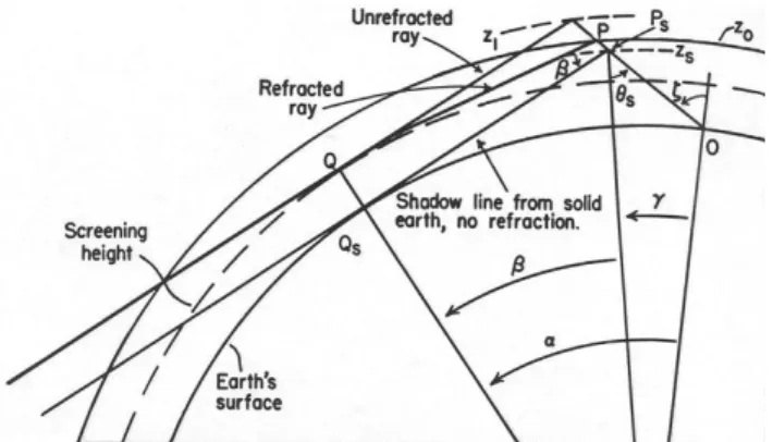
26 Figure 9. A reproduction from Chamberlain (1961). Two-dimensional geometry of twilight scattering. The incident ray that passes just above the screening height, h0, intersects the line
of sight at height z0, where the lowering of the incident ray by refraction is also included. z0 is
called the actual shadow height. ζ is the view angle of the observer, O. zs is the apparent height, the height of the shadow from the Solid Earth with no refraction.
Fig. 9. A reproduction from Chamberlain (1961). Two-dimensional geometry of twilight scattering. The incident ray that passes just above the screening height, h0, intersects the line of sight at height z0, where the lowering of the incident ray by refraction is also in-cluded. z0is called the actual shadow height. ζ is the view angle of the observer, O. zs is the apparent height, the height of the shadow
from the Solid Earth with no refraction.
18–23 km.
LIDAR observations
9. The European Centre for Medium Range Weather Fore-cast (ECMWF) analysis concludes that there is an ex-tended area of low enough temperatures for PSC’s to be formed between Scandinavia and Svalbard, consistent with the ground-based observations and the data from OSIRIS.
10. LIDAR measurements from the Koldewey Station in
Ny- ˚Alesund provide evidence for the occurrence of
PSCs within this area of cold temperatures from both the 7 and 9 of December 2002.
11. The PSC layer was measured to be in the altitude range 23–27 km, which in vertical extension corresponds to a fairly thick cloud, at most half a pressure scale height. 12. As seen from the increased depolarization values of the
LIDARS, the PSC’s contained crystalline particles. The low temperatures from the ECMWF even suggest that PSC type II clouds are formed.
Note that the obtained depolarisation values together with the cold stratospheric temperatures rules out the possibility that the event is caused by aerosols as reported by Gerding et al. (2003). It is also worth mentioning that mid-latitude
LIDAR observations from Kuehlungsborn (54◦N, 12◦E)
de-tected PSC type II conditions in early December, 2002. (Pri-vate communication Gerding, IAP).
6 Analysis of red−sky
The data-sets, when taken together, suggest that the red-sky phenomenon was related to the occurrence of PSC dis-tributed over a relatively large geographical area. First we
1600 F. Sigernes et al.: Atmospheric studies by optical methods
27 Figure 10. Two scenarios for the red-sky enigma: (A) PSC Cloud-to-Cloud scattering mechanism and (B) PSC twilight illumination.
Fig. 10. Two scenarios for the red-sky enigma: (A) PSC Cloud-to-Cloud scattering mechanism and (B) PSC twilight illumination.
note the obvious facts: it should have been completely dark
at LYR as the sun was always 10.5◦or more below the
hori-zon. Second, the presence of solar Fraunhofer and terrestrial absorption features clearly identify the source of the light as sunlight that has passed near to the surface of the Earth.
Since we know that the sunlight was bent around the Earth, we speculate that the mechanism may be one of two possible processes. The first candidate, illustrated in Fig. 10 (Panel A), is PSC cloud-to-cloud scattering where the sunlight is
piped around the Earth by a PSC located close to 68◦N, to
a second PSC located at 73◦N. It is this second, illuminated
PSC that is observed from LYR. The second candidate, il-lustrated in Fig. 10 (Panel B), is the direct illumination of a
PSC located at 73◦N by Rayleigh scattered twilight. Both of
the mechanisms considered here require that PSC occur from
73◦N to LYR.
The spectral colour of the red-sky is easily explained by the extinction of sunlight by Rayleigh scattering and ozone absorption. Figure 11 shows the modelled spectrum at LYR at 10:00 UT on 6 December 2002 using the cloud-to-cloud scattering process. A detailed description of the radiative transfer model is given by Lloyd et al. (2005). The
fig-28 Figure 11. Modelled spectral intensity of scattered sun light as viewed from Longyearbyen (78°N, 15°E) 10:00 UT on 6. Dec., 2002. Fig. 11. Modelled spectral intensity of scattered sun light as viewed from Longyearbyen (78◦N, 15◦E) 10:00 UT on 6 December 2002.
ure only shows atmospheric extinction along the path length and does not include any calculations for the cloud to cloud scattering cross-sections. The calculation uses the dry air, Rayleigh scattering, cross-sections reported by Bates (1984), the extended MSIS-90 neutral atmosphere (Hedin, 1991), the UGAMP ozone model (Li and Shine, 1995) and solar spec-trum by Kurucz et al. (1984). We have not modelled the
molecular absorption features due to O2 or H2O. It is
read-ily evident from Fig. 11 that only sunlight at wavelengths greater than 600 nm are reaching LYR and the shape of the spectrum seems to be in qualitative agreement with the MSP and spectrograph data. The optical depths implied by Fig. 11 are dominated by the Rayleigh extinction along the path from
the PSC at 73◦N to LYR. Since this path is common to both
proposed mechanisms the colour of the spectrum is not very useful for distinguishing between the two mechanisms. Cloud-to-cloud mechanism
The PSC cloud-to-cloud mechanism derives its inspiration from the fact that the red-sky was observed for 5 h from 7:30 UT to 12:30 UT. If we assume the red-sky is due to a lower latitude PSC bathed in sunlight then we can
imme-diately calculate that the cloud must between 68◦N−69◦N
at 27.5◦E as this is the only location between 20–25 km that
sees the sun for the 5 h between 7:30 UT and 12:30 UT. This model is quite appealing in that the bright, lower latitude cloud is southeast of LYR which is where the brightest sig-nal is seen and will naturally produce the brightest sigsig-nal at 10:00 UT. A crude, order of magnitude, estimate of the sig-nal brightness at LYR can be made by assuming the PSC at A and B have a vertical extinction of 0.01 which is completely scattered and that to an order of magnitude much of the scat-tering goes into the forward scatter direction and that the PSC at 68◦N supports a solid angle of approximately 5.9◦ by 5.9◦ (or 0.01 steradians) from B. Using these assumptions and
F. Sigernes et al.: Atmospheric studies by optical methods 1601 reading the value at 700 nm off Fig. 11 we find that the signal
at 700 nm at LYR is 1.0×109×0.01×0.01×0.01=1 kR/nm.
Clearly, this value is in order of magnitude agreement with observations and significantly better agreement could be eas-ily achieved by adjusting the various free parameters. PSC twilight illumination
The second mechanism is the illumination of a PSC at 73◦N
by a twilight signal. This model is very similar to the Cloud-to-Cloud mechanism except that lower latitude PSC is re-placed by sunlight which is Rayleigh scattered off the atmo-sphere. This is a relatively complex calculation which we shall leave for another time but it is sufficient to note that the Rayleigh extinction of the lower atmosphere is comparable, in order of magnitude, to the extinction of the lower latitude PSC in the Cloud to Cloud mechanism and hence can direct comparable amounts of light around the Earth to the PSC at 73◦N.
However the PSC twilight illumination model does have
several difficulties. The twilight model will produce the
brightest signals very close to the horizon while the maxi-mum signal was observed 12 deg from the horizon. In addi-tion the signal would peak when the sun was due south of the PSC at 10:30 UT while the signal actually peaks half an hour earlier at 10:00 UT. Indeed one would expect the brightest re-gion to follow the sun and steadily move from the southeast through South and into the South-West during the course of the day if the PSC had any longitudinal extent. Hence one has to assume with this model that instrumentation at LYR saw the longitudinal edge of the PSC.
The final problem with the twilight illuminated cloud is that it is probably not a rare enough occurrence. If the red-sky only required one PSC just south of LYR during the win-ter months then you might expect to witness them much more frequently than you actually do.
7 Concluding remark
The red-sky observed from Svalbard on 6 December 2002 is identified to be scattered solar light originating from type
II Polar Stratospheric Clouds (PSC) located at about 73◦N
South East of Longyearbyen − between Svalbard and Scan-dinavia. The altitude was 18–23 km up in the Stratosphere.
Two hypotheses that are able to explain the red-sky phe-nomenon in terms of sunlight scattered around the Earth are presented. Both models require PSC at latitudes north of
73◦N which scatter the light into the instrumentation at LYR.
The first model, which we feel fits the observations quite well, is PSC cloud to cloud scattering with employs a
sec-ond lower latitude PSC located at 68◦N, 27.5◦E to scatter
direct sunlight to the more northern PSC. The second model
involves the twilight illumination of the PSC at 73◦N. Both
models are able to direct the correct, order of magnitude, amounts of light but without more information on the ac-tual PSC composition, geographical extent and more com-plex modelling it is difficult to clearly pick one model over
the other. A more detailed model including multiple PSC scattering is given by Lloyd et al. (2005).
Acknowledgements. The Auroral station in Adventdalen is owned by the University of Tromsø. The University Courses on Svalbard (UNIS) operates the station. We deeply appreciate the support of the Optical group at the Geophysical Institute, University of Alaska, who owns most of the instruments used in this study. The ECMWF analysis was kindly provided to us by F. Baumgarten at ALOMAR and by P. von der Gathen at AWI.
Topical Editor O. Boucher thanks two referees for their help in evaluating this paper.
References
Bates, D. R.: Rayleigh scattering in air, Planet. Space Sci., 32(6), 785–790, 1984
Chamberlain, J. W.: Physics of the Aurora and Airglow, Academic Press, New York and London, 1961.
Fastie, W. G.: A small plane grating monochromator, J. Opt. Soc. Am., 42, 641, 1952a.
Fastie, W. G.: Image forming properties of the Ebert monochroma-tor, J. Opt. Soc. Am., 42, 647, 1952b.
Gerding, M., Baumgarten, G., Blum, U., Thayer, J. P., Fricke, K.-H., Neuber, R., and Fiedler, J.: Observations of an unusual mid-stratospheric aerosol layer in the Arctic: possible sources and im-plications for polar vortex dynamics, Ann. Geophys., 21, 1057– 1069, 2003,
SRef-ID: 1432-0576/ag/2003-21-1057.
Hauke, T.: Scientific expedition “Life in ice”, August 2002-August 2003, Observations at Kinnvika (80◦3’N, 18◦12’E) Svalbard, Nordaustland, final report, 1. October 2003, Technical University of Hamburg-Harburg, Hamburg, Germany, 2003.
Hedin, A. E.: Neutral atmosphere empirical model from the surface to lower exosphere MSIS90, J. Geophys. Res., 96, 1159–1172, 1991.
Koop, T., Carslaw, K. S., and Peter, T.: Thermodynamic stability and phase transitions of PSC particles, Geophys. Res. Lett., 24, 2199–2202, 1997.
Kurucz, R. L., Furenlid, I., Brault, J., and Testerman, L.: Solar Flux Atlas from 296 to 1300 nm, National Solar Observatory Atlas No. 1, 2nd ed., 1984.
Lloyd, N. D., Degenstein, D. A., Sigernes, F., Llewellyn, E. J., and Lorentzen, D. A.: A mechanism for the red-sky enigma: Duct-ing of sunlight by Polar Stratospheric Clouds, Ann. Geophys., in press, 2005.
Li, D. and Shine, K. P.: A 4-Dimensional Ozone Climatology for UGAMP Models., UGAMP Internal Report No. 35, April 1995, 1995.
Muller, M., Neuber, R., Beyerle, G., Kyro, E., Kivi, R., and Woste, L.: Non-uniform PSC occurrence within the Arctic polar vortex, Geophys. Res. Lett., 28, 4175–7178, 2001.
Pedersen, T.: Mystisk fenomen: Opplyst polarnatt forundrer forskerne, Svalbardposten, no. 49, 54, 2002.
Poole, L. R. and McCormick, M. P.; Airborne lidar observations of Arctic polar stratospheric clouds: Indications of two distinct growth stages, Geophys. Res. Lett., 15, 21–23, 1988.
Schreiner, J., Voigt, C., Kohlmann, A., Arnold, F., Mauersberger, K., and Larsen, N.: Chemical analysis of polar stratospheric cloud particles, Science, 283, 968–970, 1999.
1602 F. Sigernes et al.: Atmospheric studies by optical methods
Sigernes, F., Shumilov, N., Deehr, C. S., Nielsen, K. P., Svenøe, T., and Havnes, O.: The Hydroxyl rotational tem-perature record from the Auroral Station in Adventdalen, Svalbard (78◦N, 15◦E), J. Geophys. Res., 108(A9), 1342, doi:1029/2001JA009023, 2003.
Tabazadeh, A., Jensen, E. J., Toon, O. B., Drdla, K., and Schoeberl, M. R.: Role of the stratospheric polar freezing belt in denitrifica-tion, Science, 291, 2591–2594, 2001.
Toon, O. B., Tabazadeh, A., Browell, E. V., and Jordan, J.: Analysis of lidar observations of Arctic polar stratospheric clouds during January 1989. J. Geophys. Res., 105, 20, 589–20, 615, 2000. Voigt, Ch., Schreiner, J., Kohlmann, A., Zink, P., Mauersberger, K.,
Larsen, N., Deshler, T., Kr¨oger, C., Rosen, J., Adriani, A., Cairo, F., Di Donfrancesco, D., Viterbini, M., Ovarlez, J., Ovarlez, H., David, Ch., and D¨ornbrack, A.: Nitric Acid Trihydrate (NAT) in Polar Stratospheric Clouds, Science, 290, 1756–1758, 2000.