Validity of the unidirectional propagation model: application to laser-driven terahertz emission

PAPER • OPEN ACCESS

Validity of the unidirectional propagation model:

application to laser-driven terahertz emission

To cite this article: J Déchard et al 2017 J. Phys. Commun. 1 055009

View the article online for updates and enhancements.

Related content

Effects of multiple ionization in atomic gases irradiated by one- and two-color ultrashort pulses

P González de Alaiza Martínez, A Compant La Fontaine, C Köhler et al.

-Ultrashort filaments of light in weakly ionized, optically transparent media L Bergé, S Skupin, R Nuter et al.

-Modeling and simulation techniques in extreme nonlinear optics of gaseous and condensed media

M Kolesik and J V Moloney

PAPER

Validity of the unidirectional propagation model: application to

laser-driven terahertz emission

J Déchard1 _{, A Nguyen}1_{, P González de Alaiza Martínez}2_{, I Thiele}2_{, S Skupin}3 _{and L Bergé}1 1 _{CEA, DAM, DIF, F-91297, Arpajon, France}

2 _{Univ. Bordeaux—CNRS—CEA, Centre Lasers Intenses et Applications, UMR 5107, F-33405, Talence, France} 3 _{Institut Lumière Matière, UMR 5306 Université Lyon 1—CNRS, Université de Lyon, F-69622, Villeurbanne, France} E-mail:[email protected]

Keywords: unidirectional pulse propagation equation, terahertz pulse generation, wave equation, Maxwell-fluid model

Abstract

The Unidirectional Pulse Propagation Equation

(

UPPE

) is often used to compute the forward

component of ultrashort light pulses in nonlinear materials. While its accuracy has frequently been

reported for many applications in ultrafast optics, its validity can be questionable for ionizing pulses,

in particular in the frequency domain below the electron plasma frequency w

pe

. Inaccuracy of the

UPPE

model in this frequency range may be detrimental to, e.g., a correct description of laser-driven

terahertz emission. Here we demonstrate, analytically and numerically, that over long enough

propagation paths, the one-dimensional solutions of both

UPPE

and the full wave equation match in

the entire spectrum, including the spectral range

w



w

pe

. Our

findings confirm the reliability of the

UPPE

solutions for a wide class of propagation problems.

1. Introduction

The propagation of a scalar electromagneticfield in(1+1)-dimensional geometry obeys the wave equation (WE) derived from Maxwellʼs equation [1]:

¶ _E-_c-¶_E=_{Q E ,( ) ( )1}

z t

2 2 2

whereE z t( , )represents the electricfield propagating along the z-axis, c is the speed of light in vacuum and

( )

Q E is the response function that determines the linear and nonlinear properties of the material. In a centrosymmetric medium hosting free and bound electrons, this function decomposes as

m m

= ¶ + ¶

( ) ( )

Q E 0 tJ 0 t2P, 2

which involves the plasma current density (J z t, )and the macroscopic polarization (P z t, ). The latter quantity includes the nonlinear polarization,_P = c( )_E

NL 0 3 3, with c( )3 representing the third-order susceptibility assumed to be instantaneous.0and m0are the electric permittivity and the magnetic permeability in vacuum, respectively. For simplicity, we shall neglect linear gas dispersion in the forthcoming analysis. At moderate laser intensities and on short time scales, ion motion can be neglected. In the non-relativistic limit the electron current density reads as n ¶ +J J= e ( ) m N E, 3 t c 2 e e

wherenc, e,N z te( , )and meare a phenomenological collision rate, and the electron charge, density and mass,

respectively. In equation(3) the increase of free electrons is governed by the source equation

¶tNe=W E(∣ ∣)(Na-N ,e) ( )4

whereW E is a(∣ ∣) field-dependent photoionization rate and Nais the initial density of neutral atoms.

Generally, solving full Maxwell models accounting for multiple ionization processes as well as optical and plasma nonlinear effects is computationally expensive when simulating long propagation ranges as, e.g., in the

OPEN ACCESS

RECEIVED

28 July 2017

REVISED

5 September 2017

ACCEPTED FOR PUBLICATION

15 September 2017

PUBLISHED

13 December 2017

Original content from this work may be used under the terms of theCreative Commons Attribution 3.0 licence.

Any further distribution of this work must maintain attribution to the author(s) and the title of the work, journal citation and DOI.

context of ultrashort pulsefilamentation. Therefore, reduced models such as the Unidirectional Pulse Propagation Equation(UPPE) [2] are often preferred, assuming that the forward propagating component of the laser electric field conveys the major part of the energy and its coupling to the backward propagating component is negligible [3,4]. TheUPPEthen describes the so-called‘forward’ pulse component, propagating along positive longitudinal coordinates(z>0). Expressed in(1+1 dimensions, it governs the Fourier-transformed electric) fieldE z,˜( w)as

w w w ¶E z˜( )- kE z˜( )= ˜( ) ( ) kQ z , i , 1 2i , , 5 z

where tilde symbol refers to the Fourier transform:

ò

w = w -¥ +¥ ˜ ( ) ( ) ( ) f z, f z t, e d ,i t t 6

for an integrable function f andk=w c. Equation(5) is used in ultrafast nonlinear optics to describe light pulses with ultrabroad spectra[5] and in higher dimensions it can describe pulse diffraction associated with transverse wave numbers k⊥through the formal changek2k2-k^2[6].

The solution to the partial differential equation(1) is commonly advanced in time from a couple of initial/ boundary conditions on E and its derivative. In contrast, equation(5) only requires the incident field value

=

( )

E z 0,t and it is solved along the longitudinal directionz>0. Equation(5) may be refound from an easy factorization of equation(1), expressed in Fourier domain as [7–9]

¶ - ¶ + =

( z ik)( z ik E) ˜ Q˜. ( )7

Assuming weak enough nonlinearities, thefieldE˜is decomposed as the sum of(quasi) linear forward (+) and backward(−) modes, =E˜ E˜+eikz +E˜-e-ikz. Substituting the previous quantities into equation(7), applying the approximation on the backward propagator: ¶ +( z ik E) ˜+eikz »2ikE˜+eikz, and conjecturing that bothE˜andQ˜ contain essentially the part corresponding toE and˜+ Q˜+, we then arrive to equation(5). In this simple derivation, the amplitudeE+is supposed to be slow compared to eikz. This assumption is not necessary if more involved projection techniques are employed and if the PDE(1) is treated as an inhomogeneous second-order ODE [3,4]. A pending issue about the solutions of equations(5) and (7) is thus their equivalence in the whole spectrum under the formal substitution ¶ +z ik2ik. This equivalence is implicitly assumed a priori when one uses aUPPEmodel.

Proving this statement a posteriori, by computing explicit solutions of these two models, remains to be done. Over the past decade, the increasing potential of terahertz(THz) radiation has stimulated intensive efforts to develop efficient sources based on the ionization of gases by ultrashort laser pulses [10,11]. In order to properly calibrate dedicated experiments, nonlinear propagation codes have to be particularly accurate in assessing the low-frequency part of the pulse spectrum. Different experiments and plasma conformations(e.g., micro-plasmas) have been recently examined, for which relevant THz emissions in frequency ranges below the electron plasma

frequency were reported[12–14]. So far, however, the validity of theUPPEapproach has received no numerical confirmation in this specific spectral range, which is often accessed in laser-driven THz experiments [15].

To highlight more this problematics, let us consider for a moment the elementary situation where the electron density is constant, as met in a preformed homogeneous plasma. Usually, solving equation(1) needs both initial and boundary conditions onE z t( , ), the evolution of which is monitored by the dielectric function that characterizes the mediumʼs response to the electric field. In such a plasma with negligible collisions, the dielectric function expresses as( )w = -1 w2_pe w2_{, wherew ºe N ( m)}

pe

2 2

e 0 e is the electron plasma frequency andω is any Fourier frequency of the electromagnetic wave. When a monochromatic wave with frequencyω is incident on a vacuum-plasma boundary, only the fraction with real wave number

w w w

=( )( - )

kT c 1 pe2 2 1 2is transmitted into the plasma[16]. Frequency components with w wpeare evanescent and vanish over the plasma skin depth. So, for Fourier componentswwpe, the incident pulse is mainly reflected and we expect this spectral range to damp out in the transmitted pulse along the propagation path, consistently. In contrast, for theUPPEmodel, plasma opacity is not present. This can be better appreciated when looking at the linear modes of the two equations forNe=const., namely,

w ~ ⎛ - w ⎝ ⎜ ⎜ ⎞ ⎠ ⎟ ⎟ ˜( ) ( ) E z k c k z , exp i 1 pe 8 2 2 2 for equation(1), and

w ~ ⎡ - w ⎣ ⎢ ⎢ ⎛ ⎝ ⎜⎜ ⎞_⎠⎟⎟ ⎤ ⎦ ⎥ ⎥ ˜( ) ( ) E z k c k z , exp i 1 2 9 pe 2 2 2

for equation(5). Obviously these two linear solutions do not match, in particular in the domain w wpe. The WE solution(8) vanishes exponentially as z exceeds about one plasma skin length dpeº c wpe[17]. Accordingly, theUPPEsolution(9) can in principle hold in the frequency range wwpeonly. In current applications, however, in which wpevaries through the time variations of the electron densityN te( ), UPPE is supposed to be valid in the entire frequency range.

Whereas the solving for equation(1) can be performed exactly for a constant plasma frequency [16], the same problem becomes tricky when Q is a nonlinear function of E. This situation applies to a number of important issues in nonlinear optics and plasma physics[18,19]. Here, we report that, surprisingly, both solutions to equations(1) and (5) become generically identical when the plasma is self-generated in time by the laser pulse. In this paper we indeed show that the THz pulse spectra andfields, when they are described either by a full Maxwell-fluid model—encompassing both backward and forward propagations—or by itsUPPE

approximation—modeling only the forward wave—match as the pulse propagates over distances larger than the plasma skin depth and its dynamics is mainly driven by the nonlinearities.

The paper is organized as follows: we derive in section2exact analytical solutions for the twoWEandUPPE 1D models describing the secondaryfields produced inside a collisionless plasma. In the framework of a perturbative approach,WEandUPPEsolutions are shown to converge for long enough propagation distances. In section3we display numerical evidence by means of our 1DUPPEandMAXFLUcodes that over distances

d

>

z pe, bothWEforward andUPPEsolutions indeed match in the THz spectral range and therefore provide similar THzfields. This statement is established for two-color femtosecond pulses and few-cycle single-color pulses as well, at intensities privileging Kerr or plasma responses. Section4concludes our investigation. Appendixdescribes the numerical implementation of theUPPEandMAXFLUcodes.

2. The analytical solution

For technical convenience, we ignore collisional effects(n c 0). Equations(1) and (5) have the plasma

dispersion~w2_pe w2_{contained in the response function Q. The input laser profile at z = 0 is a two-color} Gaussian pulse reading in time domain as

 w w f = = ⎡ - - t + - t + ⎣ ⎢ ⎤ ⎦ ⎥ ( ) ( ) ( ) ( ) E t z I c r e t r e t , 0 2 1 cos cos 2 , 10 t t L 0 0 2 ln 2 0 8 ln 2 0 2 L 2 2 L 2

where I0is the mean pump intensity,tLis the full-width-at-half-maximum(FWHM) duration of the fundamental pulse(the second harmonic has half pump duration), r denotes the relative intensity ratio of the second harmonic andf is the relative phase between the two harmonics. One chooses a fundamental wavelength of l = 10 μm related to the carrier wave frequency w0º2pn0=2p lc 0, and an intensity ratio of =r 0.1 (two-color pulses) or 0 (single-color pulses). The interaction gas is argon at ambient pressure.The ionization rate

(∣ ∣)

W E is given by the well-known quasi-static tunnel(QST) rate

a b = ⎡ -⎣ ⎢ ⎤_⎦⎥ (∣ ( )∣) ∣ ( )∣ ∣ ( )∣ ( ) W E t E t exp E t , 11

where the constantsα and β depend on the ionization potential of the gas [20,21]. More complex rates describing multiple ionization events could be implemented as well[22]. These will be employed when investigating the highest intensity levels.

Because of the complex nonlinearities involved, we apply the same perturbation approach as in[23]. We decompose E into an unperturbed laserfield, EL, and an induced perturbation(secondary field), dE, namely,

d

= +

E EL Ewith d E EL, so that the nonlinearity Q reduces to an inhomogeneous source term only evaluated on the laserfield. Using equation (1) one obtains

¶ - ¶ = (c2 2z t2)EL 0, (12) w d ¶ + ¶ ¶ - ¶ - = [(c z t)(c z t) 2pe] E c Q E ,2 ( L) (13) w c = + ¶ ( ) ( ) ( ) c Q E2 E _tE . 14 L pe2 L 3 2 L3

Here, the perturbation dE contains the THz wavefield, which can be extracted by means of a suitable frequency filtering. The electron plasma frequency wpeis a function of time through its dependency onN z te( , ). In the tunnel ionization regime, the electron density increases steplike and produces THz radiation by coupling with the high-frequencyfieldE zL( -ct)[6]. In the framework ofUPPE(equation (5)), the perturbation instead obeys

w d

- ¶ ¶ + ¶ - =

[ 2 t(c z t) 2pe] E c Q E2 ( L). (15) Equations(13) and (15) must be solved with appropriate initial/boundary conditions. Looking for solutions propagating forward, it is natural to introduce the change of variables x =z-ct , s=t, transforming thereby

theWEandUPPEfor the perturbation dE into w d ¶ ¶ - ¶ -x = [ ( c ) ] E c Q E( ) ( ) WE : s 2 s pe2 2 L, 16 w d ¶ ¶ - ¶ -x = [ ( c ) ] E c Q E( ) ( ) UPPE : s 2 2 s 2pe 2 L, 17

respectively. It is important to notice that ELis only a function ofξ and thereby Neandwpe2 , computed on the same laserfield, only depend on ξ too. Our initial conditions for the WE read

dE s( ,x=0)=dE s( =0,x)=0, (18) yielding no constraint on the spatial derivatives. The pulse is sited in the half-planez<ct (x < 0 for causality

reasons) and enters the plasma region at time t=0. To satisfy the requirements (18), the input pulse (z=0) is positioned in the plasma domain at x_peak= - c2p tL(see insets of figures1(d) and (e)). Such boundary conditions offerflexibility to treat bothUPPEandWEsolutions in the same analytic framework. However, they differ from the inputs used in the numerical scheme of theUPPE1DandMAXFLU1Dcodes discussed inappendix. Therefore, we shall have to propagate over long enough distances  tc L 2, ensuring the full development of the nonlinearities, in order to perform quantitative comparisons between the perturbedfields dE and their

numerical counterparts. These boundary conditions also differ from those used in[23], where the progression of the laser pulse towards the plasma was described and the source term Q was tuned to zero forz<0in this reference.

For theWE, we now apply the Laplace transform ( )f p =

ò

+¥ f s( )e-psds

0 onto equation(16) to get

w x d x - + ¶ -x = [ p cp ( )] E c Q( ) ( ) p 2 . 19 2 pe 2 2

After some algebra wefind straightforwardly

ò

d x x x x x x x x x x x = ¢ + - ¢ ¢ ¢ + - ¢ ¢ x ⎡ ⎣ ⎢ ⎢ ⎤ ⎦ ⎥ ⎥ ( ) ( ) ( ) ( ) ( ) E s c Q cs G J G c cs , 2 2 , , 2 d , 20 WE 0 1

where J1is the Bessel function of thefirst kind and

ò

x x¢ = w x x¢ ( ) ( ) ( ) G , _pe2 u du 21

is positive(x < 0 andx¢x). In the original frame variables, this solution expresses as

ò

ò

ò

d x x w w x x = - ¢ _x+ - ¢ x + - ¢ ¢ -¢ -¢ ⎡ ⎣ ⎢ ⎢ ⎤ ⎦ ⎥ ⎥ ( ) ( ) ( ) ( ) ( ) ( ) E z t c Q z ct u u J c u u z ct , 2 _d 1 d d , 22 z ct z ct z ct WE 0 pe 2 1 pe 2

and its spectrum is obtained after taking Fourier transform in time t. Applying the same treatment to equation(17), we get

w x d x - + ¶ -x = [ p cp ( )] E c Q( ) ( ) p 2 2 2 , 23 pe 2 2 yielding

ò

ò

ò

d x x w w x x = - ¢ _x - ¢ x - ¢ ¢ -¢ -¢ ⎡ ⎣ ⎢ ⎢ ⎤ ⎦ ⎥ ⎥ ( ) ( ) ( ) ( ) ( ) ( ) E z t c Q z u u J c u u z , 2 _d 2 d d . 24 z ct z ct z ct UPPE 0 pe 2 1 pe 2

From afirst glance, equations (22) and (24) only differ by their linear kernel

x x x x x ¢ = + - ¢ - ¢ - ¢ + - ¢ ⎡ ⎣⎢ ⎤⎦⎥ ( ) ( ) ( ) ( ) K c z ct G z ct J cG z ct z ct 2 , 1 , , 25 WE 1 1 2 x x x x x ¢ = - ¢ - ¢ - ¢ - ¢ ⎡ ⎣ ⎢ ⎤ ⎦ ⎥ ( ) ( ) ( ) ( ) K c z G z ct J c G z ct z 2 , 2 , . 26 UPPE 1 1 2

As theUPPE/WEpulses advance in the(z t, )plane, the integration variable x¢ can cover all values from 0 to

x¢_min = - ct0 max, tmaxbeingfixed by the boundary of the time window (tmax=3.3ps here). BothUPPEandWE solutions converge towards each other at coordinates satisfyingz ∣z-ct∣> ¢∣ ∣x , as this condition assures thatKUPPE( )x¢ KWE( )x¢. This requirement can indeed be understood from applying simple Taylor expansions in the argument z+ct- ¢ »x 2z (z+ct) (2z)of theWEsolution wheneverzx¢, whereas 2 z- ¢ »x 2 in thez UPPEsolution in the same limit. These behaviors show that theUPPEsolution is missing a dependency in the(z+ct)propagation variable associated with a backward component. Applying

the second inequalityz ∣z-ct in the previous approximations leads to the convergence of the two∣ solutions.

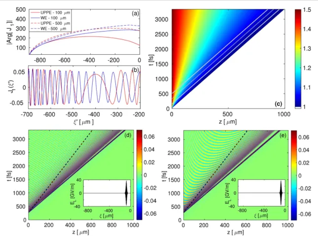
This property is reflected by figure1(a), which plots the argument of the Bessel function for a two-color 50 fs Gaussian pump pulse with 150 TW cm−2intensity. Here, the pulse region extends over x¢ <∣ ∣ 100μm and we can observe the convergence of the two Bessel arguments when the distance z is increased from 100 to 500μm. Concerning their potential discrepancies, one can observe that, at large times( x¢ >∣ ∣ 100μm), the plasma frequency wpeis constant, so thatG z( -ct,x¢ =) w2pe(x¢ - +z ct). The oscillations in theWE/UPPEsolutions are then dictated by those of the Bessel function J1. At times corresponding to x¢ » -600μm and z=100 μm,

these oscillations relax on the plasma period asJ X1( WE)~t-1 2sin(wpet c)in theWEsolution. In contrast,

( )

J X1 UPPE relaxes to the function~t-1 2sin(wpe 2t c), which develops slower oscillations around the maximum values of the Bessel arguments. Figure1(b) thus displays evidence of a minimum frequency smaller than wpein theUPPEsolution, whose value increases with z until reaching the electron plasma frequency.

To get more insight into the convergence dynamics, we may also consider a much simpler situation by assuming a constant inhomogeneity Q. With the help of equations(22) and (24), this yields the ratio

d d = -+ ⎛ ⎝ ⎜ ⎞_⎠⎟ ( ) E E z ct z ct 1 1 2 , 27 WE UPPE

which can be useful to understand the differences induced by the linear propagators. Figure1(c) shows

equation(27) as a function of z and t. The lower-right part >(z ct), in which our solutions are not defined, is set to zero for causality reason. BothWEandUPPEsolutions converge as long asz ∣z-ct , which includes the∣ laser region. In contrast, the same solutions depart from each other in the sharper limitctz. Let us now

imagine that, in the vicinity of the pulse head, the source term Q has a certainfinite extent, schematically delimited by the two grey solid lines infigure1(c). TheWEandUPPEsolutions converge near the laser head, where they are dominated by the nonlinearities computed on the laser profile. In the opposite domain, the

Figure 1.(a) Arguments of the Bessel function J1for theWEsolution(22) (blue curves) and theUPPEsolution(24) (red curves) for

different distances z and at the upper bound =t tmax=3.3ps of the temporal window. w ( )pet increases in time according to the QST

rate(11) for a two-color Gaussian pulse (1 μm + 0.5 μm) with 50 fs FWHM duration and 150 TW cm−2peak intensity.(b) The functionJ X1( )for theWEsolution(blue curves) and theUPPEsolution(red curves) at z=100 μm. The plasma frequency is reached at x¢ » -600_{μm. (c) (}z t, )map of the ratio dEWE dEUPPEas defined by equation (27) with constant source term Q. The grey dotted

line identifies the location of the laser peak at x=x_peakand the grey solid lines delimit the domain of the laser pulse.(d and e) (z t, ) maps of the full analytical solutions(d) equation (22) and (e) equation (24) with a non-constant source term driven by the same

two-color 50 fs pulse. Insets show the input pulse in the plasma domain x < 0. The black dashed lines delimit the convergence domain of theUPPEandWEsolutions, which increases with the coordinate z.

solutions are mainly driven by their linear propagators that behave differently over large times. However, the larger the propagated distance z, the broader the convergence domain, which spans a cone in the(z t, )plane(see blue area infigure1(c)). This is confirmed by figures1(d) and (e) that detail the field amplitudes in the(z t, )

plane computed from the complete expressions(22) and (24). One can see that theUPPEfield contours differ from theWEcontours in the spatio-temporal domainctz. In particular, a hyperbolic distribution occurs,

associated with the longer periods offigure1(b) and with the fact thatUPPEdoes not admit pulse components varying with z+ct. Nevertheless, the solutions achieve the same dominant component near the nonlinearity region, where they mutually converge and whose area grows with z(see figures1(d) and (e) where convergence is reached inside the cones delimited by black dashed lines).

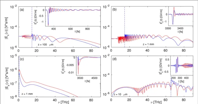
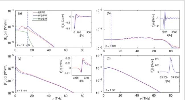
Figures2(a) and (b) show some examples of analyticalUPPE/WEspectra andfields for a two-color Gaussian pulse with FWHM duration of 50 fs, 150 TW cm−2overall intensity. The nonlinearities consist of plasma generation alone. Here and in the following the THzfields shown as insets are computed from an inverse Fourier transform ofd ˜Ein the frequency windownºw p2 90 THz. The plotted propagation distances are

z=100 μm and z=1 mm. One can observe that (i) the spectral region n<npeºwpe 2pbecomes depleted as

z increases,(ii) the minimum frequency marking theUPPEspectrum,nmin, increases in turn, and(iii) in the rear part of the pulse(beyond the laser head) theUPPElinear mode consistently develops longer periods(see inset of figure2(a)).

At smaller intensity( =I0 50TW cm−2) and with zero phase angle (f = 0), the Kerr response is expected to be a key player[24]; so we now include it. A typical Kerr-plasma spectrum at weak intensity is illustrated in figure2(c), where the low plasma frequency,n = 0.53pe THz, highlights the lesser contribution of photoionization and a parabolic spectral shape characterizes the Kerr signature in the band of higher THz frequencies(n »10-20 THz) [11]. For a mean pump intensityI0=1PW cm−2, in contrast, several electrons

can be extracted from their atom. In this high intensity regime, the ionization of the successive electron shells of argon is described by the multiple-ionization model built in[22] and based on a field-dependent cycle-averaged rate computed from the Perelomov–Popov–Terent’ev (PPT) theory [25]. At short propagation distances, unlike theWEsolution, theUPPEspectrum is not peaked at the plasma frequency n » 55pe THz, but it develops spectral oscillations in the regionn<npe, as expected(figure2(d)). At larger distances, discrepancies are amplified (not shown), because dE starts to break the underlying hypothesis of our perturbative approach, d E EL, as the perturbation itself produces optical frequencies w( 0, 2w0, ...)through the nonlinearities, e.g., the

photoionization. Since the optical pump pulse is not depleted along propagation, our formalism cannot assure a proper conservation of the electromagnetic energy. As a validity criterion we consider that our analytical solution stops to hold whenever the spectral intensity of dE at optical frequencies becomes comparable to ~75% of the laser spectral intensity. Such limitations are of course absent in the results of the full numerical

simulations, as can be inferred from, e.g.,figure6.

Figure 2. Spectra at(a) z=100 μm and (b) z=1 mm plotted from the analytical solutions (22) (WE, blue curves) and (24) (UPPE, red curves) for a two-color Gaussian pulse with mean pump intensity of 150 TW cm−2and FWHM duration of 50 fs interacting with argon. Note the oscillations in theUPPEspectrum fornnpeand the growth in nminas z increases. Same quantities at(c) z=1 mm

3. Numerical results

Our theoretical expectations are tested by running theMAXFLU1DandUPPE1Dcodes, whose respective numerical schemes are detailed inappendix. For both codes the input condition at z=0 is the two-color Gaussian pulse defined above by equation (10). The pump intensity is alternatively set to 50, 150 and 1000 TW cm−2in order to investigate various ionization degrees. The phase anglef is valued as f = 0 to enhance the Kerr effect in the 50 TW cm−2case and p 2 otherwise[24]. For Gaussian pulses with moderate laser intensity, from 50 to 150 TW cm−2, and undergoing single ionization, we employ the QST rate(11). Consistently with section2, when dealing with 1 PW cm−2pulses, multiple ionization will be described from the multi-ion model of[22] employing the field-dependent PPT ionization rate.

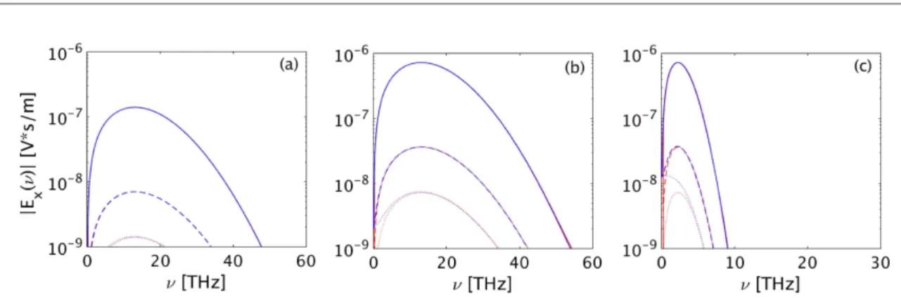
To start with, only the Kerr response is accounted for_[n =₃c( ) ₄ _c = ´_{1 10}- _{cm W}-_]

2 3 0 19 2 1 and wefirst

ignore plasma generation( =Ne 0) and collisions. Figures3(a) and (b) show the spectra of the THz fields produced in argon by a 50 fs two-color pulse with 1μm fundamental pump wavelength at increasing

propagation distances, when using theUPPEand theMAXFLUcodes. Although theWEandUPPEspectra may not perfectly match over the shortest propagation distances, e.g., z=10 μm, an excellent agreement is found at further distancesz50μm for both intensities. These simulations show that, in the absence of plasma generation, bothWEandUPPEsolutions match in the whole spectral domain over relatively short distances »10μm. This property is independent of the pulse duration, which has been counterchecked by another simulation using longer pump duration, t = 300L fs(see figure3(c)). Here, the twoUPPEandMAXFLUspectra match again over distances less than the pulse length∼90 μm. Minor early discrepancies are linked to small differences in the initialization of the numerical codes. The convergence speed between theWEandUPPEspectra driven by a Kerr response alone thus does not depend on the distance propagated over the pulse length tc L. This behavior is rather logical, as the Kerr nonlinearity is just treated as a perturbation in the source term Q and does not impact the frequency range of the linear modes in equations(8) and (9).

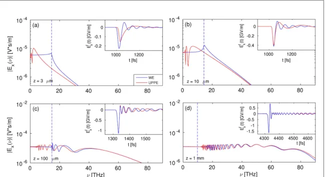
Next, infigure4, only plasma generation is taken into account, similarly tofigures2(a) and (b). So, the Kerr response and collisions are set equal to zero. The selected intensity level isI0=150TW cm−2. When the

backward-propagation operator is dropped out, the fundamental linear modes beating at the electron plasma frequency wpeare lost and no plasma opacity is allowed, which results in the development of oscillatory components in the frequency rangen <npeof theUPPEspectrum. This is consistent with the linear mode of equation(9) that admits non-zero frequency components in the rangewpe 2 wwpe. In contrast, the MAXFLUspectrum is dominated by plasma current oscillations, which prevail as long as the propagation distances remain of a few plasma skin depths(here, dpe= 3.3 mm ), as evidenced by figure4(b). Over longer distances, however, bothUPPEandMAXFLUspectra merge in the rangen>npe, as photocurrents become the dominating source in the THz generation process. Out off the laser head, long oscillations over longer times proceed from the Bessel function discussed above. Besides the good agreement between our analytical solutions shown infigures2(a) and (b) and the numerical solutions of figures4(c) and (d), we can observe that:

• At large times the field oscillations are slower for theUPPEsolution than for theWEsolution(see insets). The oscillation frequency increases as the optical path is augmented.

Figure 3. THz spectra at z=10 μm (dotted curves), z=50 μm (dashed curves) and z=1 mm (solid curves) from theUPPE1Dcode (red curves) and theMAXFLU1Dcode(blue curves) for the intensities (a) 50 TW cm−2and(b) 150 TW cm−2, using a two-color 50 fs Gaussian pulse with zero phase difference.(c) Same for a 300 fs two-color Gaussian pulse with 150 TW cm−2intensity. Only the Kerr effect is taken into account.

• Whereas, as expected, the spectral regionn <n_peisflat in the forwardWEsolution from z=3 μm, theUPPE spectrum develops oscillations from a minimum frequencynminthat increases with the propagation distance z.

• Convergence is almost reached at z=1 mm. The equality nmin=npe(associated to the plasma response of the inputfield) is met at z=1 cm and spectra match for all frequencies (not shown).

For comparison,figures5(a) and (b) show the same quantities when including the Kerr response of argon and electron-neutral collisions with the averaged rate n = 1 190c fs−1=5.3 ps−1. At 150 TW cm−2intensity, one reports a comparable matching rate between the two spectra andfields, being even sped up by the damping of oscillations at low frequencies<10THz and the decrease of the current density in time. Indeed the collision term damps the free electron current in equation(3) and thus bothUPPEandMAXFLUsolutions are also damped to zero over long times(190fs) beyond the laser head. The green curve shows the backward spectrum collected atz= -10μm from the vacuum-plasma interface in theMAXFLUsimulation. This spectrum occupies the regionnnpe, as expected[5,23], since it is emitted by plasma current oscillations over the plasma skin depth. This backward spectrum remains unchanged over propagation in vacuum.

Similar properties of matching can be refound between the solutions of the two models for pulse

configurations favoring either a weaker plasma response (thus a more efficient Kerr effect) at smaller intensities or a stronger plasma response achieved at higher intensities. Figures5(c) and (d) display the evolution of the same two-color pulse having an input intensity of 50 TW cm−2. The pulse is undergoing an effective Kerr response combined with plasma generation in argon. The corresponding plasma frequency is very weak,

n = 0.53pe THz, which is related to a long plasma skin depthd  90pe μm. Even at rather weak spectral

amplitudes, theWEandUPPEspectra andfields approach to each other over distances exceeding far this depth, at least from 1 mm, which confirms the important role of the plasma skin depth in the matching process. The spectral shape follows its analytical counterpart plotted infigure2(c) for z=1 mm. The numericalUPPE/WE spectra merge from z=5 mm until perfectly overlapping at z=1 cm (figure5(d)).

In the opposite range of pulse intensities,I0=1PW cm−2, the peak plasma density increases and a much

shorter plasma skin depth—d » 0.75pe μm for n » 65pe THz as imposed by the incident pulse—should lead to a quicker merging between theUPPEandWEsolutions. Matching is indeed achieved at about z=50 μm, i.e., over a few tens ofdpe(see figures6(a) and (b)). The optical field distortions induced by self-steepening and plasma generation are plotted as inset infigure6(b). They also show a good agreement between theWEandUPPE models at distances>10μm. The spectral distributions and THz field amplitudes (inset of figure6(a)) still reasonably agree with those computed at z= 10 μm from our analytical solution (figure2(d)). Besides, for the same high intensity level, it has been recently shown that photocurrents could be the main player for single-color

Figure 4. THz spectra andfields (see insets) at different propagation distances computed from theUPPE1Dcode(red curves) and the

MAXFLU1Dcode(blue curves) for a two-color 50 fs Gaussian pulse with 150 TW cm−2intensity:(a) z=3 μm (corresponding to almost one plasma skin depthdpe), (b) z=10 μm, (c) z=100 μm, and (d) z=1 mm. Vertical dashed lines indicate n=npe.

pulses, provided that the pulse duration be short enough, i.e., few-cycle[13]. For this purpose, figures6(c)–(e) show two spectra computed from a 1μm Gaussian pump pulse with 8 fs FWHM duration at 1 PW cm−2 intensity and evolving from z=8 μm (d » 1pe μm). Again theUPPEandWEspectra nicely approach to each other in the rangen >npefromz»100μm (not shown) and they overlap in the whole spectral range

atz»1 mm.

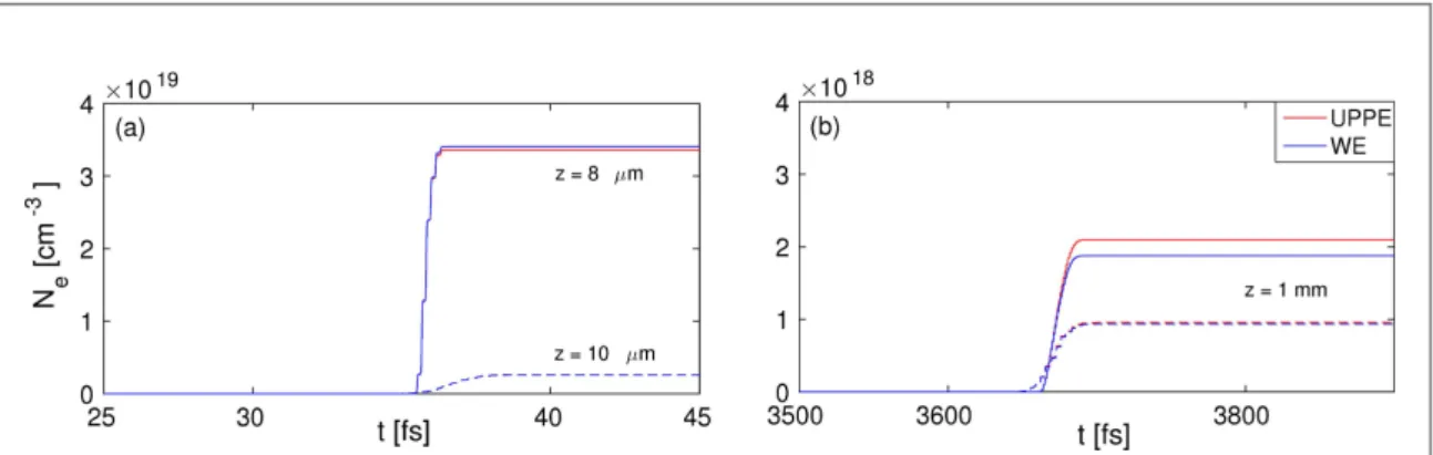
In order to illustrate the influence of the electron dynamics that can vary through laser distortions, figures7(a) and (b) finally show the electron density corresponding to figures5(a), (b) and6(c). Between the

Figure 5. Same as infigure4with same color plotstyle but with the Kerr term and electron-neutral collisions included forI0=150

TW cm−2at(a) z=10 μm, (b) z=1 mm and =I0 50TW cm−2at(c) z=1 mm, (d) z=1 cm. In (a) the green curve plots the backward spectrum collected atz= -10μm.

Figure 6. THz spectra with 1 PW cm−2laser intensity at(a) z=10 μm and (b) z=50 μm for a two-color 50 fs Gaussian pulse computed from theUPPE(red curves) andMAXFLUcodes(blue curves). Insets show the THz field at z=10 μm and the overall laser_{field at z=50 μm. (c–e) THz spectra and fields for a single-color (1 μm) Gaussian pulse with 8 fs FWHM duration} interacting with Ar at 1 PW cm−2intensity.(c) THz spectra at z=8 μm (dashed curves) and z=1 mm (solid curves). (d, e) Corresponding THzfields. Laser field patterns are shown as inset. Vertical lines point out to n=npe(with corresponding

two plotted distances, one reports for the 8 fs pulse with 1 PW cm−2peak intensity a decrease by half the maximumfield value resulting in one decade decrease in the electron density. For comparison, the 50 fs pulse with 150 TW cm−2peak intensity keeps comparable density levels. The matching distance of theUPPE/ WEsolutions for those two configurations then become similar: at z=1 mm, the 8 fs pulse with 1 PW cm−2 peak intensity has almost the same charge level as the 50 fs pulse with 150 TW cm−2peak intensity, and has thus a comparable plasma skin length(d = 3.8pe versus 5.4μm) at this distance. The two skin depths only differ from each other by a factor ~ 2 and, therefore, the twofields display comparable convergence speed between the two models. This justifies that the number of skin depths needed for matching the two solutions is not universal, as it also depends on the changes in the electron density induced by the distortions of the laserfield along propagation. Similar behaviors could be reported from longer (300 fs) pulses (not shown).

4. Conclusion

In summary, we have derived one-dimensional analytical solutions describing both bidirectional(WE) and unidirectional(UPPE) propagating light pulses by means of a perturbative approach. Structural differences between theWEandUPPEsolutions have been explored thanks to those analytical solutions, especially the shape of the THz spectra over mm-range propagation distances. The convergence between both solutions in the(z t, )plane has been examined from direct numerical computations integrating Maxwell-fluid equations

and the unidirectional pulse propagation model. Even if discrepancies in the linear propagators occur at large times beyond the laser head( ct z), theUPPEsolution matches itsWEcounterpart in the(z t, )region where the nonlinearity is effective. The extent of the convergence region increases with the propagation distance. Numerical simulations covering a wide range of pulse configurations confirm that, over a propagated distance larger than some plasma skin depths, theUPPEand Maxwell-fluid solutions

superimpose to one another. As a result,WEandUPPEspectra match remarkably well over all the spectrum, including the rangewwpe.

To conclude, we demonstrated that, in a one-dimensional geometry, theUPPEmodel, which only governs the forward pulse component, is able to provide similar spectra to a bidirectional Maxwell-fluid model over distances where Kerr nonlinearities as well as photocurrents drive THz pulse generation. Further studies should aim at testing this property in full 3D propagation geometries.

Acknowledgments

JD and LB thank Arnaud Debayle for fruitful discussions on the analytical solutions. This work was supported by

the ANR/ASTRID Project ‘ALTESSE’ # ANR-15-ASTR-0009 and performed using HPC resources from

GENCI(Grant # A0010506129 and # A0020507594). SS acknowledges support by the Qatar National Research Fund through the National Priorities Research Program(Grant # NPRP 8-246-1-060).

Appendix. The 1D

UPPE

and

MAXFLU

codes

TheUPPE1D code solves equation(5) coupled with the fluid equations (3) and (4) propagating over the optical axis z. A second-order accurate split-step scheme allows us to separate the linear and the nonlinear parts of the

Figure 7. Electron density computed from theUPPE1Dcode(red curves) and theMAXFLU1Dcode(blue curves) for an 8 fs pulse with 1 PW cm−2peak intensity(solid lines, single color), and a 50 fs pulse with 150 TW cm−2peak intensity(dashed lines, two colors) at (a) z_{=8 μm and z=10 μm, and (b) z=1 mm.}

UPPE equation[26]. The linear part (propagation) is solved exactly in the Fourier space as follows:

w w w

+ D = D

˜( ) ˜( ) [ ( ) ] ( )

E z z, E z, exp ik z , A.1

wherek( )w =w c. Then, the nonlinear contribution, including the Kerr terms, ionization and absorption

losses, are advanced over one spatial step Dz according to the equation  c m w w ¶ + ¶ = - - + ⎡ ⎣ ⎢ ⎛ ⎝ ⎜ ⎞ ⎠ ⎟⎤ ⎦ ⎥ ⎡_⎣⎢ ⎤_⎦⎥ ( ) ( ) ( ˜( ) ˜ ( )) ( ) ( ) E t c E t c J J 2 2 , A.2 z t 3 3 1 0 loss

where -1means inverse Fourier transform,Jlossrefers to a loss current due to photoionization, usually negligible in laser–gas interactions. The left-hand side of equation (A.2), which accounts for Kerr polarization, is first discretized in time by finite volumes at time step j ( = Dt j t) as

¶ = -D [F+ - F- ] ( ) E t 1 , A.3 z j j 1 2 j 1 2

where Fj 1 2+ refers to the numericalflux between two neighboring cells, j and +j 1, of the grid. Following the well-known Godunovʼs method [27], the numerical flux is given here by

c F+ = + ( ) ( ) c E 2 , A.4 j 1 2 j 3 1 2 3

whereEj 1 2+ accounts for the solution to the Riemann problem at the intercell +j 1 2[28], which aims at solving the advected solution constrained by two constant states indexed by j and +j 1on both sides of the intercell. In this case, the solution to the Riemann problem is straightforward: withc( )3 _{0, atfirst-order of} accuracy, one has to take simplyEj+1 2=Ej. To achieve second-order accuracy, we do a linear reconstruction of { }Ej following the Essentially Non-Oscillatory technique[28]:

= + D + ( ) E E 2 , A.5 j j j 1 2

whereDjcompares the downwind difference(Ej+1-Ej) and the upwind difference ( -Ej Ej 1-) and retains the lower value in modulus. Limiting the slope in this way allows us to avoid Gibbs oscillations when optical shocks induced by self-steepening occur[29]. With the second-order numerical flux, we can rewrite equation (A.2) as:

m w w ¶ = -D F+ - F- - + - ⎡ _{ } ⎣⎢ ⎤⎦⎥ [ / / ] ( ( ) ( )) ( ) E t F c J J 1 2 , A.6 z j j j j 1 2 1 2 1 0 loss

which is easily solved by the second-order Runge–Kutta method. Using this discretization, provided that c( )3 _is weak enough, the maximum spatial step given by the Courant–Friedrichs–Lewy (CFL) stability condition of equation(A.3) isD_z =_{2c t}D (₃c( )_E )

max 3 02 , with E0denoting the input amplitude of the laserfield. This step is

much larger than the spatial steps needed to obtain accurate solutions of equation(A.2) as well as those requested to integrate theWEmodel. Long propagation distances can then be simulated in reasonable amount of

computational time with the UPPE approach.

The Maxwell-fluid code, namedMAXFLU1D, is based on afinite volume scheme solving the WE (1) and fluid equations(3) and (4) in time. This set of equations is re-expressed in the conventional conservative form of a nonlinear hyperbolic system, e.g., for the transverse(x-polarized) field ºE Exthrough the electric displacement Dx: m ¶_D + - ¶_B = -_(J +_{J ), (A.7)} t x 0 z y x x 1 ,loss - = +c ( ) ( ) Dx Ex E .x A.8 01 3 3

This nonlinear hyperbolic system is treated numerically by splitting the advection part(source terms set equal to zero) and the evolution part (source terms included but with zero derivative in z) at every time stepDtalong an evolution-advection-evolution algorithm. First, the evolution stage is solved by using a second-order Runge–Kutta scheme. Next, the Maxwell and Fluid advective parts, which are independent of each other, are solved overDt. For the former advection, the Lax–Wendroff scheme is chosen (second-order accurate) [30], even though some Gibbs oscillations might appear. For the latter advection stage, instead, we couple a First Order Centered scheme[28], which isfirst-order accurate, to the Lax–Wendroff scheme, following the Flux Corrected Transport approach [31]. This is necessary for treating thefluid advection; otherwise strong Gibbs oscillations may occur in the neighborhood of electron density gradients, which can render the code unstable. The calculation domain is a sliding window that moves forward at the speed of light c and, even when accounting for the Kerr-induced changes in the optical refractive index, the CFL condition of the(t z, )grid,D = Dz c t, is the standard requirement.

In theUPPE1Dcode, the THzfield driven by the laser field is 0 at z=0. One spatial step further, the laser pulse enters the medium and triggers nonlinearities, producing thus a non zero THzfield. In theMAXFLU1D code, the THzfield grows from a laser pulse crossing a vacuum-plasma interface and admits backward

contributions. Since we are interested in THz generation, one should use simultaneously afine spectral resolution and afine time step in order to correctly describe the low frequency spectrum below npeand the two-color laser pulse components including its higher harmonics generated along propagation. The time window of our simulations is, therefore, set to 3.33 ps corresponding to a frequency step ofD = 0.3 THz.n The time stepDtis tuned from l0 (128c)down to l0 (512c)leading to a spatial step ofD =z l0 128resp.

l

D =z 0 512for theMAXFLUsimulations(CFL condition) and it is fixed toD =z l0 25for theUPPE simulations. The highest resolutions used in theMAXFLUcode have been employed when it was necessary to decrease the background noise in the lowest parts of the pulse spectrum(e.g., for a Kerr response alone).

Let usfinally notice that, so far, we have neglected linear dispersion_P = c( )* _E

L 0 1 , with c( )1 representing

thefirst-order susceptibility and * standing for the convolution product in time. Linear gas dispersion can be accounted for as well through the pulse wave numberk( )w =n( )w w c becoming then a function of the

frequency-dependent refractive index_n( )w = ₁+c( )1( )w _{. In that case, theUPPEcode iterates the solution by} always using equation(A.1) for solving the linear part and by performing the substitutions c( )3 c( )3 _n(w)

0 and mc ₀cm₀ n( )w into the left-hand side and the right-hand side of equation(A.2) of the nonlinear contribution, respectively. In theMAXFLU1Dcode the only change consists in implementing the convolution product c( ) *_E

x

1 _{in the right-hand side of the equation(A.8).}

ORCID iDs

J Déchard https://orcid.org/0000-0002-9767-7012 S Skupin https://orcid.org/0000-0002-9215-1150 L Bergé https://orcid.org/0000-0002-5531-7692

References

[1] Jackson J D 1975 Classical Electrodynamics (New York: Wiley)

[2] Kolesik M, Moloney J V and Mlejnek M 2002 Unidirectional optical pulse propagation equation Phys. Rev. Lett.89 283902

[3] Kolesik M and Moloney J V 2004 Nonlinear optical pulse propagation simulation: from Maxwellʼs to unidirectional equations Phys. Rev. E70 036604

[4] Andreasen J and Kolesik M 2012 Nonlinear propagation of light in structured media: generalized unidirectional pulse propagation equation Phys. Rev. E86 036706

[5] Köhler C, Cabrera-Granado E, Babushkin I, Bergé L, Herrmann J and Skupin S 2011 Directionality of terahertz emission from photoinduced gas plasmas Opt. Lett.36 3166

[6] Babushkin I, Skupin S, Husakou A, Köhler C, Cabrera-Granado E, Bergé L and Herrmann J 2011 Tailoring terahertz radiation by controlling tunnel photoionization events in gases New J. Phys.13 123029

[7] Kinsler P 2010 Optical pulse propagation with minimal approximations Phys. Rev. A81 013819

[8] Amiranashvili S and Demircan A 2010 Hamiltonian structure of propagation equations for ultrashort optical pulses Phys. Rev. A82 013812

[9] Babushkin I and Bergé L 2014 The fundamental solution of the unidirectional pulse propagation equation J. Math. Phys.55 032903

[10] Kim K Y, Taylor A J, Glownia J H and Rodriguez G 2008 Coherent control of terahertz supercontinuum generation in ultrafast laser-gas interactions Nat. Photon.2 605

[11] Bergé L, Skupin S, Köhler C, Babushkin I and Herrmann J 2013 3D numerical simulations of THz generation by two-color laser filaments Phys. Rev. Lett.110 073901

[12] González de Alaiza Martínez P, Davoine X, Debayle A, Gremillet L and Bergé L 2016 Terahertz radiation driven by two-color laser pulses at near-relativistic intensities: competition between photoionization and wakefield effects Sci. Rep.6 26743

[13] Thiele I, Nuter R, Bousquet B, Tikhonchuk V, Skupin S, Davoine X, Gremillet L and Bergé L 2016 Theory of terahertz emission from femtosecond-laser-induced microplasmas Phys. Rev. E94 063202

[14] Shkurinov A P, Sinko A S, Solyankin P M, Borodin A V, Esaulkov M N, Annenkov V V, Kotelnikov I A, Timofeev I V and Zhang X-C 2017 Impact of the dipole contribution on the terahertz emission of air-based plasma induced by tightly focused femtosecond laser pulses Phys. Rev. E95 043209

[15] Andreeva V A et al 2016 Ultrabroad terahertz spectrum generation from an air-based filament plasma Phys. Rev. Lett.116 063902

[16] Nodland B and McKinstrie C J 1997 Propagation of a short laser pulse in a plasma Phys. Rev. E56 7174

[17] Nicholson D R 1983 Introduction to Plasma Theory (New York: Wiley)

[18] Fibich G, Ilan B and Tsynkov S 2002 Computation of nonlinear backscattering using a high-order numerical method J. Sci. Comput.

17 351

[19] Bergé L, Skupin S, Nuter R, Kasparian J and Wolf J P 2007 Optical ultrashort filaments in weakly-ionized, optically-transparent media Rep. Prog. Phys.70 1633

[20] Landau L D and Lifshitz E M 1965 Quantum Mechanics (New York: Pergamon)

[21] Thomson M D, Kress M, Löffler T and Roskos H G 2007 Broadband THz emission from gas plasmas induced by femtosecond optical pulses: from fundamentals to applications Laser Photonics Rev.1 349

[22] González de Alaiza Martínez P and Bergé L 2014 Influence of multiple ionization in laser filamentation J. Phys. B: At. Mol. Opt. Phys.47 204017

[23] Debayle A, Gremillet L, Bergé L and Köhler C 2014 Analytical model for THz emissions induced by laser–gas interaction Opt. Express22 13691

[24] Nguyen A, González de Alaiza Martínez P, Déchard J, Thiele I, Babushkin I, Skupin S and Bergé L 2017 Spectral dynamics of THz pulses generated by two-color laser_{filaments in air: the role of Kerr nonlinearities and pump wavelength Opt. Express}25 4720

[25] Perelomov A M, Popov V S and Terent’ev M V 1966 Ionization of atoms in an alternating electric field Sov. Phys. JETP 23 924 [26] Agrawal G P 2001 Nonlinear Fiber Optics 3rd edn (San Diego: Academic Press)

[27] LeVeque R J 2002 Finite Volume Methods for Hyperbolic Equations (New York, USA: Cambridge University Press) [28] Toro E F 2012 Riemann Solvers and Numerical Methods for Fluid Dynamics: A Practical Introduction (Berlin: Springer)

[29] Anderson D and Lisak M 1983 Nonlinear asymmetric self-phase modulation and self-steepening of pulses in long optical waveguides Phys. Rev. A27 1393

[30] Lax P and Wendroff B 1960 Systems of conservation laws Commun. Pure Appl. Math.13 217