Computer Science and Artificial Intelligence Laboratory
Technical Report
MIT-CSAIL-TR-2015-029
September 24, 2015
Designing a Context-Sensitive Context
Detection Service for Mobile Devices
Tiffany Yu-Han Chen, Anirudh Sivaraman, Somak
Das, Lenin Ravindranath, and Hari Balakrishnan
Designing a Context-Sensitive Context Detection Service
for Mobile Devices
Tiffany Yu-Han Chen, Anirudh Sivaraman, Somak Das, Lenin Ravindranath, Hari Balakrishnan
Computer Science and Artificial Intelligence LaboratoryMassachusetts Institute of Technology
{
yuhan, anirudh, somakrdas, lenin, hari
}@csail.mit.edu
ABSTRACT
This paper describes the design, implementation, and eval-uation of Amoeba, a context-sensitive context detection ser-vice for mobile deser-vices. Amoeba exports an API that al-lows a client to express interest in one or more context types (activity, indoor/outdoor, and entry/exit to/from named re-gions), subscribe to specific modes within each context (e.g., “walking” or “running”, but no other activity), and specify a response latency (i.e., how often the client is notified). Each context has a detector that returns its estimate of the mode. The detectors take both the desired subscriptions and the current context detection into account, adjusting both the types of sensors and the sampling rates to achieve high ac-curacy and low energy consumption. We have implemented Amoeba on Android. Experiments with Amoeba on 45+ hours of data show that our activity detector achieves an accuracy between 92% and 99%, outperforming previous proposals like UCLA* (59%), EEMSS (82%) and Sociable-Sense (72%), while consuming 4 to 6× less energy.
1. INTRODUCTION
Inferring a mobile user’s context (i.e., properties of the user’s activity and location) is a useful service for a wide range of ubiquitous mobile applications [18, 19, 17, 1, 4, 2]. Several papers have been published on detecting user ac-tivity and location-based attributes. Despite this significant work, no previous service optimizes its detection strategy by taking into account exactly what the client is interested in. For example, a background application that wakes up once a day when the user is active should consume lesser energy than a health application that logs the user’s walk-ing/running calorie expenditure throughout the day. Yet, no systems that we are aware of explicitly take into account such client needs when determining their sensing strategy. This paper describes Amoeba, a service that exploits client input to provide accurate and energy-efficient context-sensing service.
Amoeba provides three context detectors as shown in Ta-ble 1: (1) activity, which determines if the user is static, walking, running, biking, or driving; (2) indoor/outdoor, which determines whether the user is inside or outside a build-ing; and (3) geofences, which determines if the user has
en-Context detectors/types Modes Sensors Activity Static, Walking, Running,
Biking, Driving Accelerometer,GPS WiFi, Indoor-Outdoor Indoor, Outdoor WiFi
Geofence Set of geofences GPS, WiFi, GSM, Ac-celerometer
Table 1: The context detectors in Amoeba. tered or exited one of a set of named location-based regions. Amoeba is extensible to allow other context-sensitive detec-tors, which could reuse the implemented sensor processing pipeline.
Each of these three context types has multiple modes (i.e., multiple possible states), but the user can be in only one mode at any time. This restriction simplifies the API, and provides opportunities to reduce energy. A client subscribes to one or more contexts and to one or more modes within each context. For example, a background tasking applica-tion could subscribe to “walking” or “running” in the activity context, and to “outdoor” in the indoor/outdoor context; the results may be used to log the total time or distance covered by the user while walking or running outdoors.
Amoeba incorporates the concept of context-sensitive con-text detection in depth and repeatedly applies two themes in its design and implementation:
1. Its detectors determine the sensors to use and the sen-sor sampling rates taking client subscriptions into ac-count. For example, if the client is interested in walk-ing or runnwalk-ing, the sensor samplwalk-ing rates are different from if the client is interested in biking or driving. 2. Its detectors determine the sensors and sampling rates
taking the current mode into account. For example, the geofence detector uses its distance from the nearest geofence in deciding which sensors to sample. In addition to the idea of context-sensitive sensing, and an API with mutually-exclusive subscription modes, we com-pare Amoeba’s activity detector with three prior systems [20, 26, 17] and show that it consistently consumes lower en-ergy and provides better accuracy. We have open-sourced Amoeba’s Android implementation athttps://github.com/ yuhan210/ada-android.
2. RELATED WORK
We discuss prior work on activity detection, energy-efficient activity abstractions, and localization.
2.1 Activity Detection
There have been a number of systems that focus on de-tecting a user’s activity. TransitGenie [23] uses data from the accelerometer, WiFi, and GPS to distinguish walking from driving. Zheng et al. [28, 29] infer transportation mode us-ing GPS traces. Closest to our work is Reddy et al.’s work from UCLA [20] (which we will call UCLA* in this paper) that uses GPS and accelerometer readings for activity infer-ence. However, each of the prior approach heavily relies on GPS, a sensor that consumes significant energy and does not work indoors. Hemminki et al. [8] proposed a transport-mode detector based on accelerometer readings. It obtained impressive results by estimating the periods of acceleration and deceleration. However, this approach might not general-ize to activities with variable acceleration/deceleration pat-terns, such as biking. Amoeba uses similar accelerometer features proposed in [20, 8, 11], but goes beyond and lever-ages client’s input. Besides, Amoeba also works even with uncertain availability of sensors, and dynamically switches power-hungry sensors off to conserve battery.
2.2 Energy-Efficient Activity Abstractions
Systems such as Sociable Sense [17], Jigsaw [11], and EEMSS [26] propose adaptive sampling based on a user’s current context to achieve energy-efficiency. Amoeba uses a similar concept and focuses on providing a general con-text detection service while optimizing for each client by ex-ploiting their input subscriptions. We compare Amoeba with both SociableSense and EEMSS and find that Amoeba out-performs both systems on both energy consumption and ac-curacy. Kobe [5] focuses on balancing the accuracy and en-ergy of activity detection algorithms by dynamically deter-mining where the computation should be executed. ACE [12] detects low energy proxy activities that correlate with the activity that needs to be detected. Amoeba’s approach is complementary and can be applied to the proxy detectors in ACE.2.3 Efficient Localization
Several systems reduce the energy cost of localization us-ing a variety of techniques. Some systems [30, 11] adapt their sampling rate to reduce energy cost. A-Loc [9] uses the observation that the required location accuracy varies with location. Where possible, RAPS [13] uses historical data along with the accelerometer in lieu of GPS. CAPS [15] and CTrack [25] sequence cellular base stations to retrieve ap-proximate position. Cleo [10] offloads all GPS signal pro-cessing to the Cloud to reduce energy consumption. How-ever, it requires a modified GPS board to support offload-ing, and increases wireless energy consumption (and adds latency). EnLoc [6] allows the client to pick an energy
bud- Services
Amoeba
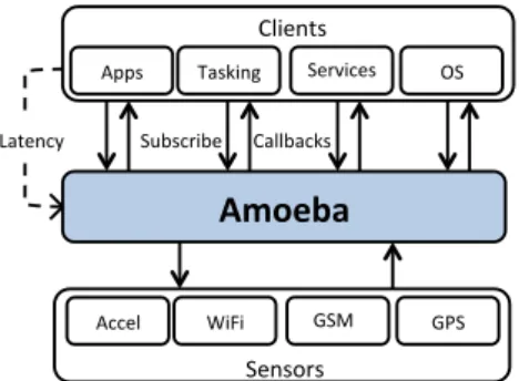
Apps Tasking Subscribe Callbacks OS Clients Latency GSM Accel WiFi GPS SensorsFigure 1: Amoeba Architecture. Amoeba takes client subscriptions and the desired response latency as input, processes sensor readings, and conveys callbacks to the clients.
get which it then uses to achieve the best accuracy subject to the energy budget constraint. Amoeba’s geofence detector can use these schemes as a black-box by deciding when to query them for location, without worrying about how they work internally.
3. SYSTEM DESIGN OVERVIEW
Figure 1 shows the design of Amoeba and Table 1 shows the sensors used by Amoeba’s context detectors. A client subscribes to one of several available modes from any of Amoeba’s context detectors. For instance, a client using movement hints to enhance the performance of WiFi (e.g. [18]) might only be interested in monitoring if the user is static or not. Alternatively, a fitness application calculating a user’s daily calorie expenditure might be interested in all five modes from the activity detector. Clients also specify the latency of detection, which specifies how often Amoeba returns its current prediction to the client. For example, a reminder ap-plication might need to notify the user within a few seconds while a trajectory logging application can tolerate a longer detection latency before it starts logging samples.
We use the term “client” rather than “application” or “pro-cess” because Amoeba’s API supports several different use cases. For example: (1) the client could be tasking applica-tions or services [19] that run in the background, triggering actions based on the activities; (2) the client could be fore-ground applications such as a Web browser or chat plug-in which adapt their user interface to the activity of the user; and (3) the client could be the operating system itself and change its behavior (e.g., turning off the screen or setting “airplane” mode) automatically. Amoeba maintains a list of clients that have subscribed to each of the modes that Amoeba’s detectors provide. It runs only one instance of a specific detector for each phone and conveys callbacks from the context detector to their respective clients.
3.1 Energy Measurement in Context Detection
To understand the power consumption of sensors on a phone, we performed experiments to quantify the power con-sumption of GPS, WiFi, GSM, and the accelerometer on0 100 200 300 400 500 600 700 0 10 20 30 40 50 60 70 80 90 Po wer (mW)
Sampling interval (secs) HTC Sensation WiFi GSM GPS Accel-fastest-50Hz Accel-game-50Hz Accel-UI-17Hz Accel-Normal-5Hz
Figure 2: Power consumption of different sensors on HTC Sensation.
mobile devices. We wrote an Android application to con-tinuously sample a sensor at a given sampling interval. For the accelerometer, we set the mode to each of FASTEST, GAME, UI, or NORMAL. In Android, some phone models stop handling sensor events when the device is sleeping. To allow Amoeba to work across models and to get a more real-istic energy consumption measurement, we used Android’s WakeLock API to keep the CPU awake. For WiFi and GSM, we used Android’s AlarmManager to schedule a periodic WiFi scan at the specified sampling interval. When the alarm fires, the Android application asks for the names and RSSIs of neighboring WiFi access points (APs) or cell towers. For GPS, we used the Android LocationManager API to specify a sampling interval. We conducted GPS measurements in an open space with good GPS reception to ensure the GPS would acquire a lock.
The power profile for the HTC Sensation is shown in Fig-ure 2 (we saw similar trends on HTC Vivid and Galaxy Nexus). We make three observations. First, there is a clear differ-ence in the power consumption of different sensors. For in-stance, at a sampling interval of 5 seconds, GSM is more than 5× as energy-efficient as GPS. Second, depending on the sampling interval, WiFi scans on the Sensation can con-sume anywhere between 16 mW and 640 mW. Third, the accelerometer power consumption increases with sampling rate since it also reflects the power consumption of a CPU polling the accelerometer for I/O at that sampling rate.
These observations guide the design of Amoeba. The first observation shows that picking which sensors to use based on the specific activities that the client is interested in will save energy. The second observation suggests that being se-lective about the sampling interval for a particular sensor is useful. Finally, because the power consumption of the ac-celerometer goes up with the sampling rate, we do not use a sampling rate higher than 20 Hz.
4. ACTIVITY DETECTOR
This detector determines which one of five activities (modes)— static (S), walking (W), running (R), biking (B), or driving (D)—a mobile device (user) is in. A client running on the
Feature
Extrac+on Extrac+on Feature
Kernel Density Es+ma+on
Label Accel traces WiFi traces
Feature Distribu1on
P (fi | A)
Latency Subscrip1ons
Accel WiFi Feature
Extrac+on Extrac+on Feature
Context-‐Sensi1ve Sampling µ, σ, pf swifi µ, σ, pf So= Fusing Smoothing (EWMA) Naïve Bayes swifi
P (Faccel | A) P (Fwifi|A)
A Ad ap t t o f ee db ac k
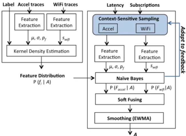
Figure 3: Amoeba processing algorithm. The labled traces are used to model the feature distributions. In the testing phase, we first use Naive Bayes to construct sen-sor distribution, and then softly fuse information from sensors together and output the smoothed prediction. mobile device may subscribe to “any subset of these activi-ties” and specify “a response interval”, L; in return, the de-tector returns its best estimate of the activity every L sec-onds. The activity detector uses data from the three-axis accelerometer, and if necessary, augmented with data from WiFi position sensors or from GPS. All of these sensors are sampled with energy-efficiency in mind, so the amount of data from GPS will be small or non-existent in many cases.
In addition to providing accurate predictions, there are several challenges that we need to address while designing a context-sensitive activity detector: (1) given client sub-scriptions and the response latency, the algorithm should determine the types of sensors to use and their sampling rates; (2) the algorithm should dynamically switch sensors on/off based on the current mode estimation; (3) since sors might be turned on/off during run-time, and not all sen-sors are available at all times (e.g., GPS is not available in-side buildings, and some phone models do not allow WiFi scanning), the algorithm should be flexible and operate un-der all circumstances.
The main contributions of our activity detector over prior schemes are: (1) a Bayesian-based processing algorithm (sum-marized in Figure 3) that softly fuses information from sors and naturally handles the uncertain availability of sen-sors, (2) an adaptive sensor sampling method that takes both the subscribed modes and the current detected mode into consideration to reduce energy consumption, and (3) a WiFi and GPS selection scheme to provide both indoor and out-door uses. The rest of this section describes these ideas.
4.1 Sensors and Features
The detection problem is a multi-label classification with the labels being S, W, R, B, and D, the five activities men-tioned above. For data collected from each sensor, the detec-tor computes feature vecdetec-tors over which the training phase
0 0.1 0.2 0.3 0.4 0.5 0.6 0.7 0.8 0.9 1 0 1 2 3 4 5 Cumulati ve probability density Peak Frequency
Static Walking Running Biking Driving
Figure 4: CDF of peak frequency. and online learning method can work.
Accelerometer. As in prior work [20], we compute the magnitude,qa2
xi+ a2yi+ a2zi, of each three-axis
accelerom-eter reading. To capture user’s movement, we compute a feature vector every T seconds. There are numerous pos-sible features one could construct and try out. We experi-mented with many possibilities, inspired by previous work on activity detection [20, 8]. These features include: mean, standard deviation, peak non-DC frequency, spectral coef-ficient at 1 Hz, 2 Hz, and 3 Hz [20], spectral entropy [11], peak power ratio [23]. We conducted controlled experiments with various combinations of the above features and empir-ically determined that the first three features above: mean (µ), standard deviation (σ), and peak frequency (pf) per-form the best. Incorporating other features or using a subset of the three features is detrimental to the prediction accuracy (see §8). Our detector therefore processes the timestamped acceleration data to produce a sequence of µ, σ, pf values, each calculated over a T -second non-overlapping window. Note that we pick T = 5 since a smaller window runs the danger that we might not have enough samples to capture key features of the movement mode.
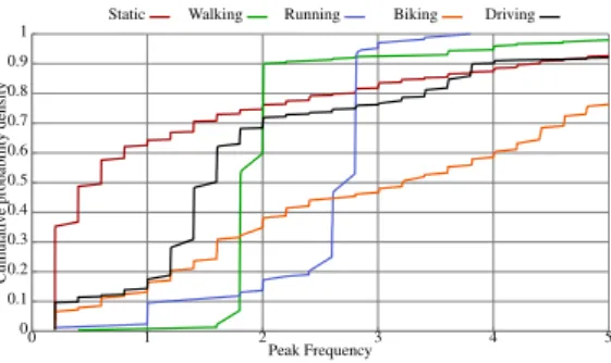
The mean and standard deviation captures the movement intensity. For example, running has the highest mean and standard deviation while static has the lowest. The peak non-DC frequency (pf) captures the idea that different activi-ties have different principal frequencies (see Figure 4, which plots the CDF of peak frequency for different activities; the sharp rise in CDF is visible for walking and running, and to a slightly lower degree for biking and driving, compared to the other activities).
WiFi. Acceleration-derived features are good at capturing activities with distinct movements, but distinguishing bik-ing from walkbik-ing, runnbik-ing, and drivbik-ing is a vexbik-ing prob-lem ([22] discusses a similar probprob-lem). Augmenting the acceleration-derived features with approximate speed esti-mates could help this distinction.
We use the similarity of observed WiFi APs and their RSSI values over successive WiFi scans to obtain a crude proxy for the user’s speed of movement. Each WiFi scan re-turns a “fingerprint”, defined as a set of (APID, RSSI) tuples. When the user’s moving at a higher speed, two consecutive fingerprints should look very different. That is, the rate of
Sensors Features
Accelerometer mean, standard deviation, peak frequency WiFi similarity between two consecutive fingerprints
GPS speed
Table 2: The features used in Amoeba’s activity detector. change of fingerprints tells us something about the rate of movement of the user. To use this idea, we need a measure of the similarity between two WiFi fingerprints. We treat each fingerprint as a vector in the space constructed by all the WiFi APs, and the RSSIs determines its direction in the space. We measure the similarity, swifi, between two WiFi fingerprints as follows:
swifi( ~f1, ~f2) = ~f1· ~f2
k ~f1k2+ k ~f2k2− ~f1· ~f2 ,
where ~fi is a fingerprint scanned at ti. 0 ≤ swifi ≤ 1, with a larger value suggestive of slower movement. As an example, consider the fingerprints f1 at time t1 equal to {(ID=1, RSSI=3), (ID=2, RSSI=5)}, and f2at time t2equal to {(ID=1, RSSI=2), (ID=3,RSSI=1)}. They are converted to (3,5,0) and (2,0,1) in the WiFi AP space, and swifi =
(3∗2+5∗0+0∗1)
34+5−6 = 336. We considered other similarity met-rics, including one from [25]; we found our metric performed better. The reason is that it more naturally handles finger-prints with partially overlapping or non-matching APs.
GPS. Incorporating accelerometer readings with WiFi might not solve all the issues. For example, rural areas have low WiFi coverage. Therefore, we use the speed measurement sgps from the GPS sensor when WiFi AP density falls be-low a threshold or when WiFi scanning is unavailable. We turn GPS off when we see good WiFi coverage to minimize energy consumption.
Table 2 summarizes the sensor-derived features.
4.2 Modeling Sensor Distributions
Armed with these features from each sensor, the next step is to model the sensor distribution and train the model. Modeling feature distributions. For each feature fiwhere fi ∈ {µ, σ, pf, swifi, sgps}, its probability density condi-tioned on an activity Ai (where Ai ∈ {S, W, R, B, D}) is P(fi|Ai). We use labeled training data and model each of them as a kernel density estimation (KDE) [16, 21] , or a sum of normalized Gaussians. Each Gaussian has the same variance h2
i and has mean equal to one of the training data samples. The parameter h is tunable to trade off between overly smoothing the data (large h) and overfitting the data (small h). We explain how we pick hi in §8 using cross-validation on the training data set.
KDE has a number of good properties for our purposes. First, it does not assume a single Gaussian and can handle multimodal distributions well. Second, the tunable band-width parameter in KDE compensates for the difference be-tween feature distributions across users/devices. Third, the model is easy to update. We can incorporate new training
samples by appending them into the current training set and simply extending the summation that computes the proba-bility density. Lastly, our experimental results show that it outperforms other algorithms such as Naive Bayes, decision tree, and support vector machine (SVM).
Constructing sensor distributions. Given P(fi|Ai), we can model the conditional probability distribution for each sensor: P(Faccel|Ai), P(Fwifi|Ai), and P(Fgps|Ai), where Faccel= {µ, σ, pf}, Fwifi = {swifi}, and Fgps= {sgps}.
However, the acceleration-derived feature vector Faccel has three components. A multi-variate conditional distribu-tion P(Faccel|Ai) is unwieldy. We use a Naive Bayes clas-sifier, which separates the components and then multiplies the conditional probabilities of the different components to-gether. However, the result may produce a zero posterior probability. We need to “regularize” the result, for which we apply a standard m-estimator [7]: given a probability mass function P(A), the probability estimate P( bA) using the m-estimator is P( bA) = NP(A)+φP(A)N+φ , where P(A) is a prior probability and φ determines how much weight we attribute to the prior P(A). We use the uniform prior, and φ = N/5 because we have five modes in all.
Note that instead of creating a feature vector with all the features and constructing P(Faccel,wifi|Ai), we model the conditional distribution for “each sensor”. We do this be-cause the former approach would weigh the acceleration data considerably higher than the WiFi or GPS data, and not al-low us to explicitly control the weight given to these two independent sensors.
4.3 Fusing Sensor Data: Soft Fusing
Our goal, of course, is to determine P(A|Faccel, Fwifi orFgps), for which we apply the Bayes’ rule:
P(A|Faccel, Fwifi) = P(FaccelP(F, Fwifi|A)P(A) accel, Fwifi) (1) Fgps and Fwifi are interchangeable, and we omit Fgps in the equation for simpler explanation. We assume that the prior distribution P(A) is known; in our implementation, we set them all to be equal. The denominator is a normaliza-tion factor that does not need to be separately determined. Assuming Facceland Fwifi are conditionally independent, which can be considered to be true given that they provide complementary movement information, we can write Eq. 1 as:
P(A|Faccel, Fwifi) ∝ P(Faccel|A)P(Fwifi|A)P(A) ∝ P(Faccel|A)P(Fwifi|A)
(2) Based on Eq. 2, we softly combine information from sen-sors and take the product of the likelihood probabilities for each activity, and obtain the posterior probability. The soft fusing technique has several good properties: (1) it helps dis-ambiguate some tricky cases. For example, if the user is
ing, the acceleration computations alone might confuse bik-ing with walkbik-ing or runnbik-ing (but not drivbik-ing), givbik-ing walk-ing (or runnwalk-ing) and bikwalk-ing comparable probabilities. On the other hand, WiFi or GPS might confuse biking with driving because they may have similar speeds, but not with running or walking. After the “soft fusing” using the product, we are far more likely to infer the correct activity; (2) soft fusing naturally handles cases such as the uncertain availability of sensors, or unsynchronized sensor data provision. For ex-ample, if WiFi scanning is not allowed on a particular phone model, we can assign P(Fwifi|Ai) to be a uniform distribu-tion, or give little weight to the WiFi likelihood probability.
The final step in the algorithm smoothes these vote results using an exponentially weighted moving average (EWMA) filter. The detector returns the activity with the highest value of the smoothed soft fusing.
4.4 Context-Sensitive Sampling to Save Energy
4.4.1 Adapt to client-specified subscriptions
To make the activity detector energy efficient, we adapt the choice of sensors and their sampling rates based on the client-specified subscription and the response interval L.
We discussed how the acceleration data performs well in detecting that the activity is static, walking, or running, and incorporating WiFi or GPS gives only marginal gains for these activities. Therefore, we use only the acceleration data when the client subscribes to any subset of these three activ-ities (S, W, R), and turn off WiFi and GPS to save energy. In other cases, we scan the WiFi or GPS sensor every L seconds to conform to the required response latency.
4.4.2 Adapt to feedback from detector
We adaptively turn off GPS, WiFi, or sample accelerome-ter at a lower sampling rate based on the feedback from the detector.
WiFi/GPS selection. WiFi AP has a lower coverage density in rural areas, and the opposite in urban areas. On the con-trary, GPS is less accurate in urban areas [14], and the oppo-site in rural areas. Since we only need one source of speed estimation, we continuously monitor the WiFi AP density and only turn on the GPS when the WiFi AP falls below a threshold (the number of neighboring APs is fewer than 2). Adaptively turn off WiFi to save energy. Similar to the concept we applied in sensor selection based on client-specified subscription, we turn WiFi off when accelerometer detects with a high probability (P(A|Faccel) > 0.8) that the activity is static, walking, or running.
Adapting accelerometer sampling rate. Increasing accelerom-eter sampling rate trades energy for better detection accu-racy [27]. We adapt the sampling rate of accelerometer using P(A|Faccel). The detector starts sampling the accelerometer at the lowest sampling rate, and then ramps up to the next higher rate (accelerometer rates are discrete) every time the accelerometer is in a fussy state – it detects the user is in
bik-ing or drivbik-ing. Besides, we never use a samplbik-ing rate higher than 20 Hz.
5. LOCATION-BASED CONTEXT
DETEC-TORS
This section describes Amoeba’s indoor-outdoor and ge-ofence detectors.
5.1 Indoor-Outdoor Detector
For the indoor-outdoor detector, the set of mutually exclu-sive modes is indoor and outdoor. To tell if a user is indoor or outdoor, we use variation in WiFi RSSI indoors and out-doors. Specifically, we employ two features of WiFi scans. First, the fraction of good AP sightings in a micro window µ . We define a sighting to be “good” if its RSSI is greater than a per-phone threshold (set to 80 for the Galaxy Nexus)1 Sec-ond, the average RSSI across all AP sightings in the same micro window µ.
To train, we sample WiFi scans at 1 Hz and set µ to 5 sec-onds. Conditioned on the user’s mode (indoor or outdoor), we fit a Gaussian distribution to each of the two features listed above.
During classification, we have four time scales of interest: (1) The developer specified latency L. (2) A sliding macro window M which is set to L. (3) A sliding micro window µ over which the two features (fraction of good APs and average RSSI) are computed. µ is set to L
2. (4) The WiFi scan interval I which is set to L/4.
To classify, we first compute both feature vectors over the micro window. Since the micro window is twice as large as the scan interval, we are likely to include at least two scans while computing both features. Next, we average the feature vectors from all micro windows belonging to the same macro window to generate a prediction feature vector Fi/o. Since the macro window is twice as large as the micro window, we typically average at least two feature vectors while com-puting Fi/o. Lastly, we use the prediction feature vector to compute the likelihood that Fi/owas observed indoor or out-door. Similar to the activity detector, we use the Naive Bayes to compute the likelihood of Fi/o, i.e., P(Fi/o|A) (where A = {indoor, outdoor}).
5.2 Geofence Detector
Geofencing is a way of marking a virtual boundary around a geographical region. Geofences are typically defined as circular regions using a center (expressed in latitude and lon-gitude) and a radius. A geofence detector monitors the loca-tion of the user and detects if the user has entered a geofence of interest. As an example, an application could let a user create a geofence on a map and trigger a notification when she enters it. Many tasking applications [1, 4, 2] have been built around geofencing.
1Per-phone calibration is required to determine a “good” threshold, but need not be repeated for every user using that type of phone.
Naive implementations of a geofence detector can either be energy-intensive or have poor accuracy. For instance, constantly sampling the GPS is not energy-efficient despite often being accurate. At the other extreme, solely using a low-power position sensor might create a lot of false posi-tives and false negaposi-tives.
Amoeba includes a geofence detector that is both accu-rate and energy-efficient. The detector uses GPS, WiFi and cellular radios (i.e., GSM) to get location samples. The ge-ofence detector adapts both the sampling interval and the lo-cation sensor to the current context of the user. If the user is far from the nearest geofence, the detector uses a low-power sensor and samples at a larger interval. As the user nears a geofence, it switches to a high power sensor and samples more frequently to check if the user have entered the ge-ofence.
As input, our geofence detector takes a list of geofences that the client subscribes to and a latency parameter (L) sim-ilar to the activity detector. The algorithm varies two pa-rameters based on the current context of the user: when to sample next (t), and which sensor to use on the next sam-pling instant (s). We set t equal to minD
maxSpeed where minD is the minimum distance between the current location and the nearest geofence accounting for the accuracy in the loca-tion sample (for example, GSM localoca-tions can have errors up to 2 miles). If the calculated t is less than L, we reset t to L (i.e. the latency of detection the client is willing to tolerate). We set a lower bound of 1 hour on the sampling interval t as a failsafe. We choose maxSpeed to be 150 miles/hour un-der the realistic assumption that the user is unlikely to ever travel faster than that speed on roads (true of the US). To set s, we look at the current value of minD. If minD is larger than the error bound of GSM (we use 2 miles as the GSM error [25]), we choose GSM. Alternatively, if minD falls between the error bounds of WiFi (we use 200 meters as the Wifi error [24]) and GSM, we sample WiFi. Lastly, if minD is less than the error bound of WiFi, we switch to GPS. As soon as we find the user inside a geofence, we trigger a call-back for that particular geofence.
When the user is inside a geofence, we use a similar tech-nique to adapt the sampling time and the sensor used (based on the size of the geofence and the distance to the next near-est geofence). As an optimization, we also use the activity detector to detect if the user is static or moving and use it to refine the next sampling time.
6. IMPLEMENTATION
We have implemented all the techniques explained in pre-vious sections in Java for Android devices. It is challeng-ing to implement an accurate continuous-senschalleng-ing mobile ser-vice. First of all, we need to achieve correct detection. Sec-ond, Amoeba’s activity detector heavily relies on accelera-tion data; intensive computaaccelera-tion on acceleraaccelera-tion data would leave little CPU time for the reception of accelerometer data. Third, because Amoeba retrieves and processes sensor data
continuously, a simple implementation would deplete the battery quickly and so care must be taken to ensure low energy overhead. In this section, we explain how we im-plemented Amoeba to ensure its correctness and minimize energy overhead.
We implemented Amoeba as a background service that continues to run even if an interested application is not run-ning in the foreground. For the activity detector, an ac-celerometer event listener continuously listens for and stores data received from the accelerometer. To output a activity prediction every response latency L, Amoeba schedules a Handler to run every L seconds and asks for accelerome-ter data from the acceleromeaccelerome-ter event listener. Using the ac-celerometer data from the last L seconds, Amoeba computes the accelerometer-derived features to obtain probability esti-mates for each activity and estimate the current activity.
However, a naive implementation fails to work because the accelerometer event listener and the Handler run in the same thread; computing the features and probability esti-mates in the Handler blocks the reception of accelerometer sensor events, causing the number of accelerometer samples in each window to vary wildly. This could be fixed by run-ning the event listener and the Handler in separate threads. But that would require synchronization of accesses to the accelerometer data shared between both threads, an error-prone operation. Instead, we let the accelerometer event lis-tener govern updates to the accelerometer-derived features and per-mode probability estimates by tracking the times-tamps on all received accelerometer data.
Mobile operating systems are designed to aggressively put the devices to sleep as soon as they become “idle”. Some phone models stop handling sensor events when the device is sleeping. To allow Amoeba to work with those phone models, we use Android’s WakeLock API to keep the CPU awake, and we explicitly remove the WakeLocks if the ser-vice is stopped to conserve battery. Lastly, since the Java library in Android does not have implementation of kernel density estimation, we used our own KDE implementation based on the one available from SciPy [3].
We used a dual-core HTC Sensation to profile Amoeba’s CPU and memory overhead during execution. Loading all the KDE models from the disk to the memory takes 6–8 seconds. However, we only need to load models the first time we start the service, and it can be done in the back-ground. The models can even be prefetched before the ser-vice starts running. Extracting all the features from all the sensors and computing the probability estimates take around 180 milliseconds, which is negligible for our applications. The memory footprint is dominated by the in-memory rep-resentation for the KDE models. In total, maintaining the models takes around 900 kB — < 0.05% of the memory for current phone models.
7. EVALUATION
We describe how we evaluate Amoeba in this section. First,
User Static Walking Running Biking Driving
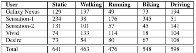
Galaxy Nexus 129 137 49 73 194 Sensation-1 234 38 176 345 51 Sensation-2 131 101 57 45 141 Vivid 74 133 114 18 104 Desire 73 54 80 67 108 Total 641 463 476 548 598
Table 3: Total activity data collected (in minutes) for each user.
we focus on data collection and how we split up the collected data into training and testing sets; then, we discuss the met-rics we use to evaluate the system.
7.1 Data Collection
We developed an Android application that collects traces of users engaged in different activities. The application col-lects sensor data by sampling the GPS at 1 Hz and accelerom-eter at its maximum sampling rate, and by scanning WiFi ev-ery second. To collect ground-truth, the user tags her current activity on a UI.
Activity dataset. We use two activity datasets: one is used to do offline comparison with other prior systems and ana-lyze our processing pipeline; the other one is to evaluate the online performance of Amoeba in a real-world setting.
(1) Our offline activity dataset spans 45+ hours and is col-lected from five users (2 females and 3 males). We call these users “Galaxy”, “Sensation-1”, “Sensation-2”, “Vivid”, and “Desire” to reflect the phone model used by each user and list the data collected from each user in Table 3. We set aside approximately 50% of 2 users’ (Galaxy Nexus, Sensation-1) data from Table 3 as the training set (we never use it during testing). To train Amoeba, we use 4-fold cross validation on this training set to determine the best value of Amoeba’s KDE bandwidths (hi) for all features. We then freeze the algorithm and evaluate it on the remaining data.
(2) Our online activity dataset is collected using our Amoeba implementation described in the previous section to provide natural activity data that occurs as part of the user’s everyday routine. Users also tags her current activity on a UI while our implementation is running at the background. We fix the response latency to 15 seconds, and assume the client is in-terested in all 5 activities. In total, we collected 11 hours of data from two testers (1 male and 1 female).
Indoor/outdoor dataset. To collect indoor/outdoor dataset, we alternate walking indoors and outdoors for roughly one minute while tagging the ground-truth at all times. We train the detector on about 30 minutes of data covering both in-door and outin-door modes collected using a Galaxy Nexus. To test, we collect another 90-minute trace with indoor and outdoor transitions.
Geofence dataset. We evaluate the geofence detector on 48000 hours of data drawn from 182 users taken from the GeoLife dataset [28, 29]. It consists of 18670 GPS traces (tracks) where a user commutes from a source to a destina-tion. The location samples on these traces are obtained using GPS. We assume that these samples have high accuracy and
hence define the ground truth of the user’s location. To sim-ulate WiFi and GSM sensors at a sampling instant, we add random noise to the GPS location according to the WiFi and GSM accuracy models [24, 25].
7.2 Evaluation Metrics
To form a continuous trace with transitions between modes, we concatenate traces together with a uniform mode transi-tion probability. We use the concatenated trace to simulate the actions of a detector on sensor data, and output two met-rics:
1. Accuracy: We measure accuracy as the fraction of time during which the ground-truth and the detector agree on an activity. We discretize the ground-truth into bins of size L seconds, where L is the response latency for that detector. For each L-second bin, we compute the set of all activities in the ground-truth and the detector’s output over that bin, replacing any activ-ity that the client hasn’t subscribed to with an X. If the detector’s output is a subset of the ground-truth in that bin, we mark it correct, else we mark it wrong. The accuracy is measured as the fraction of bins where we predict correctly.
2. Energy Consumption: We measure energy consumed in joules over the entire duration of the trace. For each sensor, we compute its energy consumption as Pi=K
i=1 (ti+1− ti)Piwhere Piis the power consump-tion of the sensor over the time interval [ti, ti+1] and K is the number of power consumption switches for sensor j over the duration of the trace. We then add up the energy consumption of all sensors. The power val-ues are derived from hardware models of each phone as described earlier in §3.
8. RESULTS
8.1 Activity Detector
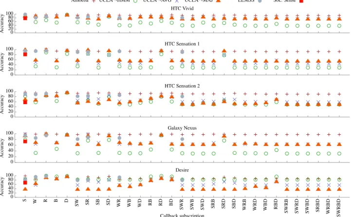
8.1.1 Accuracy and energy for all subscriptions
For Amoeba’s activity detector, a subscription is a set of activities that a client is interested in. We use five traces, the first three traces (about 8-hour long) are from Desire, Sensation-2, and Vivid. The next two traces (about 4-hour long) are from Sensation-1 and Galaxy. For each of the 31 subscriptions, we set the response latency to 15 seconds (L = 15) and plot the energy consumption and accuracy as shown in Figure 7 and Figure 6. The HTC Desire’s bat-tery cannot be removed from its enclosure which prevents us from connecting a power monitor to estimate its energy con-sumption. Hence, the energy consumption figure does not include a figure for the HTC Desire.
We first compare Amoeba against UCLA* [20]. We im-plement 3 different versions of UCLA*. The first, UCLA*-HMM, implements the algorithm as described in [20].
How-ever, it is tuned for a latency of 1 second and hence, may under-perform at higher latencies. As a remedy, we imple-ment a second version, UCLA*-MAJ, which takes a major-ity vote of UCLA*-HMM’s 15 predictions over a 15-second window. We also implement UCLA*-AVG, which averages the 15 raw feature vectors computed by UCLA* over a 15-second window and then uses the averaged feature vector to predict the transport mode. We also compare against EEMSS [26] and SociableSense [17] and only evaluate them on the sub-scriptions they are able to handle. For EEMSS, we consider biking and driving to be the same class, and train a speed threshold using our training set.
Accuracy. As shown in Figure 6, Amoeba’s activity detec-tor is more accurate than all other schemes (in some cases by up to 1.5×). Amoeba’s activity detector performs better than UCLA* because UCLA* heavily relies on GPS, which does not have good reception in urban canyons and inside build-ings. UCLA* is unable to make predictions when there’s no GPS signal, whereas Amoeba’s adaptively selects between WiFi and GPS and uses soft fusing to handle the unavail-ability of sensors. For traces with good GPS reception (e.g., Desire), UCLA* performs similar to the accuracy they re-ported, and Amoeba’s comparable to it. Amoeba’s improved accuracy relative to EEMSS is because Amoeba uses bet-ter features and distribution modeling techniques; EEMSS’s thresholding approach is not robust enough to work well across different users/devices. Amoeba’s improved accuracy comparing to SociableSense is because their learning-based duty cycling adaptation scheme picks a low duty cycling (to conserve battery) when the user is not moving, and misses many moving events. It also requires a longer time period to ramps up to a faster sampling duty cycle. On the con-trary, Amoeba is governed by the client-specified response latency.
Energy. Amoeba’s gains in energy consumption relative to the UCLA* variants are due to the sparing use of the GPS. The UCLA* variants all sample GPS frequently. In con-trast, Amoeba’s samples GPS only when the WiFi density is low and completely turns it off while detecting any sub-set of running, walking or static. Besides, since Amoeba is context-sensitive to client-specified subscriptions, Amoeba consumes lesser energy for the static, walking, and running subscriptions compared to subscriptions containing the bik-ing and drivbik-ing modes. Despite detectbik-ing many more ac-tivities than SociableSense and EEMSS, Amoeba has lower or comparable energy consumption across all subscriptions. The main reason is because Amoeba samples accelerometer at lower rate when it is certain about user’s current activity.
8.1.2 Accuracy and energy as a function of
client-specified latency
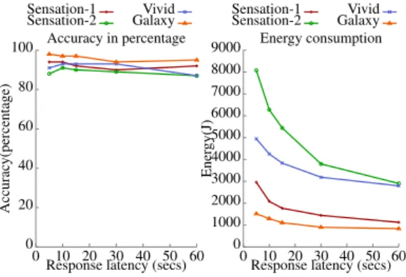
Amoeba also adapts its sensing strategy to the client-specified response latency. We test this by setting the latency to 5, 10, 15, 30 and 60 seconds and plot the resulting energy and accu-racy. Figure 5 shows that Amoeba allows the client to
trade-0 20 40 60 80 100 0 10 20 30 40 50 60 Accurac y(percentage)
Response latency (secs) Accuracy in percentage Sensation-1
Sensation-2 GalaxyVivid
0 1000 2000 3000 4000 5000 6000 7000 8000 9000 0 10 20 30 40 50 60 Ener gy(J)
Response latency (secs) Energy consumption Sensation-1
Sensation-2 GalaxyVivid
Figure 5: Energy and accuracy v.s. latency. Amoeba’s activity detector trades off promptness for lower energy consumption.
Ground Truth (%)
Static Walking Running Biking Driving
Prediction Static 98 10 0 0 5 Walking 0 80 16 0 0 Running 0 0 82 0 0 Biking 1 8 2 96 0 Driving 1 2 0 4 95
Table 4: Confusion matrices for the online performance of Amoeba’s activity detector.
off promptness of detection for lower energy consumption while maintaining the same accuracy. These energy savings are the result of adapting the WiFi and GPS sampling inter-vals.
8.1.3 Real-world online performance
Table 4 shows the real-world online performance of Amoeba’s activity detector. The accuracy is between 80% and 98%, remains high for most cases. Amoeba’s ability in detecting walking degrades in this experiment. The first reason is be-cause there’s a delay between when the user tags her ground-truth and when she starts walking. And that is why Amoeba mislabels it as static. Besides, the peak frequency feature requires the user to walk steadily in order to capture the pe-riodic behavior. In reality, users occasionally pause between strides, and fail to show a principal frequency. Besides, Amoeba occasionally mislabels running as walking, since the user could slow down while running without changing the ground-truth. Scheme µ σ pf µ, σ σ, pf µ, pf µ, σ, pf Accel 54 63 54 69 74 73 83 Accel 60 62 57 72 76 76 86 + WiFi/GPS Accel 71 68 68 78 80 87 90 + WiFi/GPS + EWMA
Table 5: % accuracy with feature subsets, all 5 call-backs. Removing even one of Amoeba’s features de-grades performance. µ, σ, and pf refer to the mean, standard deviation and peak frequency features of accel-eration data. EWMA refers to the prediction smoothing.
Scheme Amoeba Amoeba
+ 1 Hz Amoeba+ 2 Hz Amoeba+ 3 Hz Amoeba+ PPR Amoeba+ SE
Accel 83 80 79 76 60 76 Accel 86 80 79 77 63 78 + WiFi/GPS Accel 90 87 85 82 65 82 + WiFi/GPS + EWMA
Table 6: % accuracy while adding other features. Amoeba’s accuracy degrades when other features are added. EWMA refers to the prediction smoothing. 1 Hz, 2Hz, and 3 Hz refer to spectral coefficients at 1, 2, and 3 Hz respectively. SE refers to spectral entropy and PPR refers to Peak Power Ratio.
8.1.4 Deconstructing the activity detector
This section explains how we determine the set of features used in Amoeba’s activity detector. Assuming the client is interested in all activities, we evaluate all seven non-empty subsets of the three accelerometer features: mean (µ), stan-dard deviation (σ), and peak frequency (pf). For each of these subsets, we also evaluate the effect of adding and re-moving WiFi/GPS information. Finally, we evaluate the ef-fect of adding both WiFi/GPS and prediction smoothing (EWMA) on classification accuracy.
As shown in Table 5, removing any of Amoeba’s features degrades performance. And any combination of two ac-celerometer features performs better than any single feature. Furthermore, adding the speed information from WiFi/GPS using soft fusing improves accuracy from 83% to 85%, and the EWMA smoothing technique improve the accuracy fur-ther to 90%. We also tried combining Amoeba’s acceleration-derived features with other features proposed in prior sys-tems: spectral coefficient at 1 Hz, 2 Hz, and 3 Hz, spectral entropy (SE), and the peak power ratio (PPR). As Table 6 shows, augmenting µ, σ, and pf with any of other features, regardless of whether WiFi and GPS are used, the accuracy degrades.
8.2 Indoor-Outdoor Detector
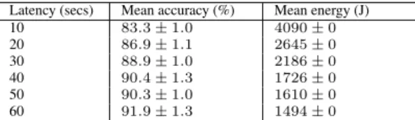
We vary the response latency between 10 seconds and 60 seconds. For latencies where the sampling rate L
4 isn’t one of the WiFi sampling intervals used in our power measure-ments, we interpolate between the nearest two neighbors. We present results in Table 7. The columns are the latency, the average accuracy in percentage and 95% confidence in-terval across 10 seeds, and the average energy consumption in Joules over the 3-hour stitched trace and 95% confidence interval across 10 seeds. The table shows how the indoor-outdoor detector effectively allows us to trade off latency of detection for reduced energy consumption and increased ac-curacy.
8.3 Geofence detector
We evaluate the accuracy and energy consumption of the Geofence detector in two parts: 1. By varying the latency parameter l and 2. by varying the number of geofences a
0 20 40 60 80 100 Accurac y HTC Vivid
Amoeba UCLA*-HMM UCLA*-AVG UCLA*-MAJ EEMSS Soc. Sense
0 20 40 60 80 100 Accurac y HTC Sensation 1 0 20 40 60 80 100 Accurac y HTC Sensation 2 0 20 40 60 80 100 Accurac y Galaxy Nexus 0 20 40 60 80 100 S W R B D SW SR SB SD WR WB WD RB RD BD SWR SWB SWD SRB SRD SBD WRB WRD WBD RBD SWRB SWRD SWBD SRBD WRBD SWRBD Accurac y Callback subscription Desire
Figure 6: Accuracy for all subscriptions. Across all subscriptions, Amoeba achieves higher accuracy than other schemes. 100 1000 10000 100000 Ener gy (J) HTC Vivid
Amoeba UCLA* EEMSS Soc. Sense
100 1000 10000 100000 Ener gy (J) HTC Sensation 1 100 1000 10000 100000 Ener gy (J) HTC Sensation 2 100 1000 10000 100000 S W R B D SW SR SB SD WR WB WD RB RD BD SWR SWB SWD SRB SRD SBD WRB WRD WBD RBD SWRB SWRD SWBD SRBD WRBD SWRBD Ener gy (J) Callback subscription Galaxy Nexus
Figure 7: Energy consumption for all subscriptions. Across all subscriptions, Amoeba consumes lower energy than other schemes. The power number for Desire is missing since its battery could not be removed from its enclosure.
Latency (secs) Mean accuracy (%) Mean energy (J) 10 83.3 ± 1.0 4090 ± 0 20 86.9 ± 1.1 2645 ± 0 30 88.9 ± 1.0 2186 ± 0 40 90.4 ± 1.3 1726 ± 0 50 90.3 ± 1.0 1610 ± 0 60 91.9 ± 1.3 1494 ± 0
Table 7: Energy and accuracy for Amoeba’s indoor-outdoor detector
client subscribes to.
For the first part, we take each trace and assume that a geofence exists at the destination of the trace. We set the radius of the geofence to 200 meters, which typically covers a block. As the user commutes from the source to the desti-nation, we simulate our geofence detector which adapts the sampling time and the sensor used. We also log the number of times we trigger GPS, WiFi, GSM sensors to compute the total energy consumption using the power measurement we collected.
Several clients are latency-insensitive and can trade-off promptness of detection for lower energy consumption. Our detector allows this tradeoff by adapting to the latency pa-rameter. As Figure 8 (left) shows, the power consumption reduces as the latency parameter increases. Compared to a naive approach that samples GPS at a constant interval, our detector consumes low energy but achieves the same ac-curacy. For example, using the power consumption values from Figure 2, if the GPS on the Galaxy Nexus were to be sampled once every 60 seconds, it consumes around 50 mW, whereas our detector consumes only 8 mW in the median.
Next, we evaluate the energy consumption of our detector by varying the number of geofences the detector looks for. To do this, we pick the top k popular locations for a given user and run the detector on all traces of that user. Figure 8 (right) shows that, as the number of geofences increases, the amount of energy consumed increases. It demonstrates how a client can tradeoff the number of geofences it wishes to detect for a decrease in energy consumption.
0 0.05 0.1 0.15 0.2 0.25 0 10 20 30 40 50 60 Po wer(W)
Developer specified latency (secs) Power vs latency 5th 25th 50th75th 95th 0 0.05 0.1 0.15 0.2 0.25 0.3 0.35 0.4 1 2 3 4 5 6 7 8 9 10 Po wer(W)
Number of subscribed callbacks Power vs number of callbacks
5th
25th 50th75th 95th
Figure 8: Geofence power percentiles. Amoeba’s ge-ofence detector consumes low energy and its energy con-sumption increases as the number of geofences increases.
9. CONCLUSION
We presented Amoeba, a context-sensitive context detec-tion service for mobile devices. Amoeba implements three context detectors that detect user’s activity, whether she is indoors/outdoors, and if a user has entered/exits a region. Amoeba exports an API to mobile clients that allows them to express their interests and specify a response latency. Amoeba leverages client’s subscriptions as well as the current context to dynamically adapt the sensors to use and their sampling rates. We evaluated Amoeba and found that it outperforms prior methods in terms of both accuracy and energy con-sumption.
10. REFERENCES
[1] Locale. http://www.twofortyfouram.com/. [2] OnX.https://www.onx.ms/.
[3] SciPy kernel density estimation.http://docs.scipy. org/doc/scipy/reference/tutorial/stats.html. [4] Tasker. http://tasker.dinglisch.net/.
[5] D. Chu, N. D. Lane, T. T.-T. Lai, C. Pang, X. Meng, Q. Guo, F. Li, and F. Zhao. Balancing energy, latency and accuracy for mobile sensor data classification. In Proceedings of the 9th ACM Conference on Embedded Networked Sensor Systems, SenSys ’11, pages 54–67, New York, NY, USA, 2011. ACM.
[6] I. Constandache, S. Gaonkar, M. Sayler, R. R. Choudhury, and L. P. Cox. EnLoc: Energy-Efficient Localization for Mobile Phones. INFOCOM ’09. [7] J. Cussens. Bayes and Pseudo-Bayes Estimates of
Conditional Probabilities and Their Reliability. ECML ’93.
[8] S. Hemminki, P. Nurmi, and S. Tarkoma.
Accelerometer-based transportation mode detection on smartphones. SenSys ’13.
[9] K. Lin, A. Kansal, D. Lymberopoulos, and F. Zhao. Energy-accuracy trade-off for continuous mobile device location. MobiSys ’10.
[10] J. Liu, B. Priyantha, T. Hart, H. S. Ramos, A. A. F. Loureiro, and Q. Wang. Energy efficient GPS sensing with cloud offloading. SenSys ’12.
[11] H. Lu, J. Yang, Z. Liu, N. D. Lane, T. Choudhury, and A. T. Campbell. The Jigsaw continuous sensing engine for mobile phone applications. SenSys ’10. [12] S. Nath. ACE: exploiting correlation for
energy-efficient and continuous context sensing. MobiSys ’12.
[13] J. Paek, J. Kim, and R. Govindan. Energy-efficient rate-adaptive GPS-based positioning for smartphones. MobiSys ’10.
[14] J. Paek, J. Kim, and R. Govindan. Energy-efficient rate-adaptive gps-based positioning for smartphones. In MobiSys, 2010.
[15] J. Paek, K.-H. Kim, J. P. Singh, and R. Govindan. Energy-efficient positioning for smartphones using Cell-ID sequence matching. MobiSys ’11.
[16] E. Parzen. On Estimation of a Probability Density Function and Mode. Ann. Math. Statist., 33(3):pp. 1065–1076, 1962.
[17] K. K. Rachuri, C. Mascolo, M. Musolesi, and P. J. Rentfrow. SociableSense: exploring the trade-offs of adaptive sampling and computation offloading for social sensing. MobiCom ’11.
[18] L. Ravindranath, C. Newport, H. Balakrishnan, and S. Madden. Improving wireless network performance using sensor hints. NSDI ’11.
[19] L. S. Ravindranath, A. Thiagarajan, H. Balakrishnan, and S. Madden. Code In The Air: Simplifying Sensing and Coordination Tasks on Smartphones. HotMobile ’12.
[20] S. Reddy, M. Mun, J. Burke, D. Estrin, M. Hansen, and M. Srivastava. Using mobile phones to determine transportation modes. ACM Trans. Sen. Netw., 6(2):13:1–13:27, Mar. 2010.
[21] M. Rosenblatt. Remarks on Some Nonparametric Estimates of a Density Function. Ann. Math. Statist., 27(3):832–837, Sept. 1956.
[22] L. Stenneth, O. Wolfson, P. S. Yu, and B. Xu. Transportation mode detection using mobile phones and gis information. SIGSPATIAL GIS, 2011. [23] A. Thiagarajan, J. Biagioni, T. Gerlich, and
J. Eriksson. Cooperative transit tracking using smart-phones. SenSys ’10.
[24] A. Thiagarajan, L. Ravindranath, K. LaCurts, S. Madden, H. Balakrishnan, S. Toledo, and J. Eriksson. VTrack: Accurate, Energy-Aware Road Traffic Delay Estimation Using Mobile Phones. SenSys ’09.
[25] A. Thiagarajan, L. S. Ravindranath, H. Balakrishnan, S. Madden, and L. Girod. Accurate, Low-Energy Trajectory Mapping for Mobile Devices. NSDI ’11. [26] Y. Wang, J. Lin, M. Annavaram, Q. A. Jacobson,
J. Hong, B. Krishnamachari, and N. Sadeh. A framework of energy efficient mobile sensing for automatic user state recognition. MobiSys ’09. [27] Z. Yan, V. Subbaraju, D. Chakraborty, A. Misra, and
K. Aberer. Energy-efficient continuous activity recognition on mobile phones: An activity-adaptive approach. ISWC, 2012.
[28] Y. Zheng, Y. Chen, Q. Li, X. Xie, and W.-Y. Ma. Understanding transportation modes based on GPS data for web applications. ACM Trans. Web, 4(1):1:1–1:36, Jan. 2010.
[29] Y. Zheng, L. Liu, L. Wang, and X. Xie. Learning transportation mode from raw GPS data for geographic applications on the web. WWW ’08. [30] Z. Zhuang, K.-H. Kim, and J. P. Singh. Improving
energy efficiency of location sensing on smartphones. MobiSys ’10.