MIPAS reference atmospheres and comparisons to V4.61/V4.62 MIPAS level 2 geophysical data sets

(1)

HAL Id: hal-00328212

https://hal.archives-ouvertes.fr/hal-00328212

Preprint submitted on 10 Jul 2007

HAL is a multi-disciplinary open access

archive for the deposit and dissemination of sci-entific research documents, whether they are pub-lished or not. The documents may come from teaching and research institutions in France or abroad, or from public or private research centers.

L’archive ouverte pluridisciplinaire HAL, est destinée au dépôt et à la diffusion de documents scientifiques de niveau recherche, publiés ou non, émanant des établissements d’enseignement et de recherche français ou étrangers, des laboratoires publics ou privés.

MIPAS reference atmospheres and comparisons to

V4.61/V4.62 MIPAS level 2 geophysical data sets

J. J. Remedios, R. J. Leigh, A. M. Waterfall, D. P. Moore, H. Sembhi, I.

Parkes, J. Greenhough, M.P. Chipperfield, D. Hauglustaine

To cite this version:

J. J. Remedios, R. J. Leigh, A. M. Waterfall, D. P. Moore, H. Sembhi, et al.. MIPAS reference atmospheres and comparisons to V4.61/V4.62 MIPAS level 2 geophysical data sets. 2007. �hal-00328212�

(2)

ACPD

7, 9973–10017, 2007 MIPAS reference atmospheres compared to V4.61/2 MIPAS data J. J. Remedios et al. Title Page Abstract Introduction Conclusions References Tables Figures ◭ ◮ ◭ ◮ Back Close Full Screen / Esc

Printer-friendly Version Interactive Discussion Atmos. Chem. Phys. Discuss., 7, 9973–10017, 2007

www.atmos-chem-phys-discuss.net/7/9973/2007/ © Author(s) 2007. This work is licensed

under a Creative Commons License.

Atmospheric Chemistry and Physics Discussions

MIPAS reference atmospheres and

comparisons to V4.61/V4.62 MIPAS level 2

geophysical data sets

J. J. Remedios1, R. J. Leigh1, A. M. Waterfall2, D. P. Moore1, H. Sembhi1, I. Parkes1, J. Greenhough1, M.P. Chipperfield3, and D. Hauglustaine4

1

EOS, Space Research Centre, Department of Physics and Astronomy, University of Leicester, Leicester, LE1 7RH, UK

2

Atmospheric Science, Space Science and Technology Department, CCLRC Rutherford Appleton Laboratory, Chilton, Didcot, Oxfordshire, OX11 0QX, UK

3

School of the Environment, University of Leeds, Leeds, UK

4

LSCE, CNRS/CEA, lOrme-des-Merisiers, 91191 Gif-sur-Yvette, France Received: 18 June 2007 – Accepted: 25 June 2007 – Published: 10 July 2007 Correspondence to: J. J. Remedios (j.j.remedios@le.ac.uk)

(3)

ACPD

Printer-friendly Version Interactive Discussion

Abstract

Reliable reference profiles and estimates of variability are a necessity for a variety of processes relating to ENVISAT including the development of key aspects and inputs for the operational processor for the Michelson Interferometer for Passive Atmospheric Sounding. MIPAS reference atmospheres have therefore been produced in two forms,

5

namely standard atmospheres for modelling and error analysis for typical atmospheric situations and the IG2 seasonal climatologies for initial guess profiles used as part of the operational processing. The reference states cover 36 species on a common altitude, pressure, and temperature grid from 0 to 120 km, and include both means and estimates of variability (maximum, minimum and one sigma values). This paper

10

describes V3.1 of the standard atmospheres and V4.0 of the IG2 atmospheres which are the current versions of the reference atmospheres. Particular attention is paid to the MIPAS operational geophysical products (pressure/temperature, H2O, O3, CH4, N2O,

HNO₃and NO₂) and to CO₂whose mixing ratio is required for the retrieval of pressure and temperature. A dynamic representation of CO2 is presented which shows the

15

presence of CO2gradients in the troposphere and the lower stratosphere.

Since these atmospheres have been produced independently of MIPAS data, it is also possible to compare the data to the MIPAS operational products and derive valu-able information on both the reference atmospheres and on MIPAS data products them-selves. This process has been performed for V4.61/V4.62 data from the year 2003 as

20

part of the MIPAS validation activity. It is demonstrated that the agreement between the MIPAS mean data and the reference atmospheres is very good in mid-latitudes and the tropics, verifying these data to first order. There is also reasonable agreement in standard deviations between the IG2 atmospheres and the corresponding sigmas calculated from the MIPAS data. Knowledge of tropospheric concentrations of CH4

25

and N₂O is used to examine the accuracy of the MIPAS data and their susceptibility to cloud effects. It is shown that for the highest accuracy, MIPAS data should be fil-tered with cloud index values of 2.5 for N2O and 3.5 for CH4. Once such filtering has

(4)

ACPD

Printer-friendly Version Interactive Discussion been performed, the MIPAS data for these species appear to be accurate to within

10% in the upper troposphere. The use of cloud index data in combination with MI-PAS data is recommended for studies of the polar winter stratosphere and the upper troposphere/lower stratosphere.

1 Introduction

5

Reference atmospheres for atmospheric gases can deliver a simple, accessible but quantitative description of the mean state of the atmosphere and likely deviations from that state. As such they are useful for a variety of purposes from inputs to radiative transfer simulations and inversion algorithms, to initial states and first order verifications for atmospheric measurements and models. The reference atmospheres described

10

here were constructed specifically within the frame of the Michelson Interferometer for Passive Atmospheric Sounding (MIPAS) to provide well-characterized sitations for de-velopment of key aspects of the retrieval process for pressure/temperature and trace gases, to provide initial guess/contaminant profile data for the operational Level 2 pro-cessing of infra-red radiance to geophysical data products and to provide atmospheric

15

concentrations for evaluation of error budgets for the data products.

Prior to MIPAS launch, existing reference atmospheres consisted of standard pro-files covering many species for typical atmosphere situations, e.g.,U.S. Standard

At-mosphere (1976), Anderson et al. (1986), or more sophisticated zonal mean clima-tologies but for restricted numbers of species and altitude ranges, e.g.CIRA(1986), or

20

advanced climatologies with error/variability estimates for specific species, e.g.,Fortuin

et al. (1998) for ozone, Chiou et al.(1997) for water vapour. For MIPAS purposes, it was desirable to include information on many infra-red active species for both standard states and seasonal climatologies on a grid from the surface to 120 km, with estimates of variability in order to cover the varying needs of the project. An initial study byEchle

25

et al. (1992) had generated typical profiles for MIPAS but the study reported here was intended to be more detailed in estimation of seasonal climatologies and standard

(5)

ACPD

Printer-friendly Version Interactive Discussion viations. In addition, it was anticipated that the MIPAS reference atmospheres should

also be more representative of the information available from the Upper Atmosphere Research Satellite (UARS) and from tropospheric monitoring of changes in source gases, particularly the anthropogenic greenhouse gases in the 1990s. With these con-siderations, it was decided that what was required for MIPAS reference atmospheres

5

were two sets of reference databases: 1) a set of standard atmospheres covering five atmospheric states encompassing broad latitudinal and seasonal variability (tropical, mid-latitude day/night, polar summer and polar winter); 2) a seasonal climatology com-prising a four season, six latitude climatology database (the “IG2 climatology or Initial Guess 2 climatology).

10

The generation of reference descriptions of the atmosphere necessarily implies that some prior knowledge of the expected state is contained within the databases. Hence the availability of these detailed MIPAS reference atmosphere databases also pro-vides an opportunity to intercompare with MIPAS data products since the reference databases are independent of MIPAS data. These enable both the reference

atmo-15

spheres to be considered for their appropriateness and the large-scale mean and sta-tistical variations of MIPAS data products to be verified. This exercise is performed in this paper for the MIPAS operational products and enables identification of mean be-haviour, statistical variability, and cloud effects. In keeping with the MIPAS validation papers in this special issue, this paper reports on results for MIPAS V4.61/V4.62 data

20

for the 2003 period.

2 The MIPAS instrument

The MIPAS instrument (Fischer and Oelhaf, 1996; Fischer et al., 2000) is a Fourier transform spectrometer (FTS) on ENVISAT employing limb sounding to obtain verti-cally resolved profiles of atmospheric infra-red emission spectra between 685 cm−1

25

(14.60 µm) and 2410 cm−1 _{(4.15 µm). Key characteristics of MIPAS include its high}

(6)

ACPD

Printer-friendly Version Interactive Discussion the mid-troposphere (or lower) to the mesopause (and into the mesosphere in some

modes) at moderately high vertical resolution, and its global coverage with true pole to pole, latitudinal sampling. Between launch and March 2004, the nominal full spec-tral resolution mode of operation for the majority of acquisitions allowed for a specspec-tral resolution of 0.025 cm−1 _{(unapodized) over the entire spectral range with only narrow}

5

gaps between the five spectral channels of the instrument. Vertical profiles in this nom-inal mode were scanned from 6 km to 68 km with a vertical spacing of 3 km in the UT and lower stratosphere commensurate with the field-of-view of the instrument. Each profile required approximately 76 s corresponding to an along-track distance of 500 km between vertical scans.

10

The essential steps in subsequent treatment of the data recorded by the instrument are transformation of the recorded interferograms to atmospheric spectra, calibration and inversion to geophysical data sets. The processing of the data to produce geo-located, radiometrically and spectrally corrected spectra at level 1b is described in

Kleinert et al. (2007). The quality of the level 1b spectra produced operationally by

15

the European Space Agency (ESA) are excellent with offsets in the calibrated spectra believed to be less than 2 nW/cm2sr cm−1 ₍_{Spang et al.}_,₂₀₀₅_{). Typical noise values}

for a single spectrum vary between 40 nW/cm2sr cm−1 at 800 cm−1 to less than half that value at 1200 cm−1and to 3 nW/cm2sr cm−1 at 2100 cm−1.

Within these spectra, the spectral signatures of more than thirty trace gases can

20

be distinguished from the immensely rich information content of atmospheric emission observed at high spectral resolution. The ESA operational processing of the data to level 2 geophysical products focusses on pressure/temperature, water vapour, ozone, methane, nitrous oxide, nitric acid and nitrogen dioxide in the altitude range from 6 to 68 km. The retrieval methodologies for the operational processor are described by

25

(Raspollini et al., 2006). It is V4.61/V4.62 data produced by this processor which is the subject of the comparisons in this paper and hence a particular focus also for the reference atmosphere descriptions. Nonetheless, in the generation of the reference atmospheres for MIPAS all the major relevant species emitting in this spectral range

(7)

ACPD

Printer-friendly Version Interactive Discussion had to be considered and estimates made for their concentrations.

3 Reference atmospheres

The construction of the MIPAS reference atmospheres was driven by the desire to have an accessible, useful description of expected atmospheric states which could be em-ployed either directly in the MIPAS operational processor or used indirectly in off-line

5

calculations related to auxiliary data or information for the processor. Standard at-mospheres representing typical atmospheric states and their latitudinal variation were more appropriate for computationally expensive operations such as microwindow op-timisation and selection, level 2 geophysical error estimation and for forward model optimisation. For initial guess and contaminant profiles within the processing itself, a

10

more climatological database was necessary which encapsulated both seasonal and latitudinal variations (the IG2 database). For both types of atmospheres, estimates of variability were an important addition to climatological data sets. Both the standard atmospheres and the IG2 seasonal climatologies were constructed to cover pressure and temperature, and concentrations of thirty six species: N2, O2, C2H2, C2H6, CO2,

15

O3, H2O, CH4, N2O, 11, 12, 13, 14, 21, H22,

CFC-113, CFC-114, CFC-115, CH₃Cl, CCl₄, HCN, NH₃, SF6, HNO₃, HNO₄, NO, NO₂, SO₂, CO, HOCl, ClO, H2O2, N2O5, OCS, ClONO2, COF2.

3.1 Sources of data

The compilation of the reference atmospheres for a large number of species was able

20

to benefit from the efforts of a number of observational and modelling studies that de-livered valuable data sets prior to the launch of ENVISAT in 2002. The zonal mean climatology for temperature was taken from the CIRA (1986) which ensured hydro-static equilibrium. Other single product climatologies utilised included the climatology ofFortuin et al. (1998) for ozone andChiou et al.(1997) for water vapour which were

(8)

ACPD

Printer-friendly Version Interactive Discussion very useful for the troposphere and upper troposphere/lower stratosphere respectively.

As part of this work also, an average tropospheric climatology of water vapour was calculated for five years of ECMWF re-analysis data (1979–1983).

Data from the UARS Reference Atmosphere Project (URAP), co-ordinated by the lead author of this publication, constituted a large element of the stratospheric

obser-5

vational data set. In this project, climatologies of major stratospheric constituents were developed from observations by instruments on the UARS launched in 1991; data from UARS instruments provided a significant observational advance in global knowledge of stratospheric constituents. The zonal climatologies were mostly calculated on both log(pressure) and theta surfaces; the theta data were mapped with equivalent

lati-10

tude also. For the log(pressure) case, standard deviations were also estimated for the monthly data sets. “Baseline” datasets were calculated for the period April 1992 to March 1993, since this provided the maximum species coverage by UARS instruments and minimised the effects of aerosol loading from the Mt. Pinatubo eruption. However, where possible, the URAP project also allowed for “extended” atmospheres which were

15

averaged over a longer period of time, and additional atmospheres which were aver-ages of data not falling within the baseline period. The extended atmospheres have been used in this study where possible. Further information on some of the URAP climatologies can be found inWang et al.(1999) andRandel et al.(1999).

Ground-based networks played a particularly important role in providing surface data

20

for tropospheric source gases such as the anthropogenic greenhouse gases including the halocarbons, and sulphur compounds. Data from the NOAA-related networks of carbon dioxide, including the GLOBALVIEW-CO2 (2006) system have been incorpo-rated as have reported observations from the AGAGE network (Prinn et al., 2000). At the time of the major part of the construction of the base information for the

refer-25

ence atmospheres, much of the data were available only up to 2000 although the IG2 carbon dioxide dataset reported here is dynamic and is updated on an annual basis. Ground-based observations have been complemented by observations of mixing ratios from aircraft measurements, e.g. as part of the NOAA Globalview project or from

(9)

ACPD

Printer-friendly Version Interactive Discussion paigns, and have been useful also in checking on maximum/minimum limits of mixing

ratios.

Model data were also input to the study and were used particularly for the sea-sonal IG2 climatologies. Stratospheric trace gas distributions were calculated using the SLIMCAT 3-D off-line chemical transport model (CTM) (Chipperfield, 1999).The

5

model uses an isentropic vertical coordinate with horizontal winds and temperatures are specified from meteorological analyses, while the vertical (diabatic) motion is cal-culated from a radiation scheme within the model. The model is coupled to a detailed stratospheric chemistry scheme, which contains a treatment of gas phase and het-erogeneous reactions. More details are given inChipperfield (1999). For the results

10

used here the model was integrated from October 1991 until March 2000 at the hor-izontal resolution of 7.5×7.5 degrees and 18 isentropic levels from 330 K to 3000 K. The model was forced using UK. Met. Office analyses (Swinbank and O’Neill,1994). Monthly mean data and standard deviations were computed from the model 5 day out-put between 23 April 1992 and 7 March 2000 with model fields interpolated (in log(p))

15

from the model isentropic levels to standard UARS pressure levels.

Tropospheric model climatologies were generated based on a complete year of data from the Model for OZone And Related Chemical Tracers (MOZART) global model. This is a three-dimensional Chemical Transport Model (CTM) of the global tropo-sphere described and evaluated by Brasseur et al. (1998) and Hauglustaine et al.

20

(1998). The model was originally developed in the framework of the National Center for Atmospheric Research (NCAR) Community Climate Model (CCM). In the version of MOZART used here (version 1), the time history of 56 chemical species is calculated on the global scale from the surface to the mid-stratosphere. The model accounts for surface emissions of chemical compounds (N2O, CH4, NMHCs, CO, NOx, CH2O, and

25

acetone), advective transport, convective transport, diffusive exchanges in the bound-ary layer, chemical and photochemical reactions, wet deposition of 11 soluble species, and surface dry deposition. This version of the model chemical scheme included 140 chemical and photochemical reactions and considered the photochemical oxidation

(10)

ACPD

Printer-friendly Version Interactive Discussion schemes of methane (CH₄), ethane (C₂H₆), propane (C₃H₈), ethylene (C₂H₄),

propy-lene (C3H6), isoprene (C5H8), terpenes (α-pinene, C10H16), and a lumped compound

n-butane (C4H10) used as a surrogate for heavier hydrocarbons. The evolution of

species was calculated with a numerical time step of 20 min for both chemistry and transport processes. The model was run with a horizontal resolution which is

identi-5

cal to that of CCM (triangular truncation at 42 waves, T42) corresponding to about 2.8 degrees in both latitude and longitude. In the vertical, the model uses hybrid sigma-pressure coordinates with 25 levels extending from the surface to the level of 3 mb.

A number of standard atmosphere profiles were also available (Echle et al.,1992;

Anderson et al., 1986) based on previous literature and these were very useful for

10

species, such as NH₃for which relatively little is known about the height profile. 3.2 MIPAS standard atmospheres

The MIPAS standard atmospheres were intended to provide a updated set of pro-files, pre-launch, for characteristic atmospheric states such as those derived by the studies of Echle et al. (1992) and Anderson et al. (1986). Its main objective was

15

to provide reference states for computationally expensive calculations in the devel-opment of the MIPAS operational processor including the selection of microwindows and occupation matrices (MW/OM) selection for the operational processor, the gen-eration of look-up tables (LUTs) for forward model calculations and error estimation. However, the atmospheres are also useful for a range of investigations from retrieval

20

algorithm development and specification to instrument design. Since the MIPAS op-erational processor is based on a latitudinal switching of associated files such as mi-crowindows and LUTs, the standard atmosphere states were also chosen to be latitu-dinal in form with different conditions for the poles (polar summer and polar winter) and a day/night form for mid-latitudes although the processor itself does not allow

25

day/night switching of auxiliary data. This resulted in five atmospheric states being represented on a 0–120 km grid with 1 km spacing: tropical, mid-latitude (day/night), polar winter and polar summer (also sigma, maximum and minimum profiles). Current

(11)

ACPD

Printer-friendly Version Interactive Discussion data versions are V3.1 for the MIPAS standard atmospheres (available for download at

http://www.atm.ox.ac.uk/RFM/rfm downloads.html). To allow for variation in the states, maximum and minimum values (extreme values) were calculated at each altitude. From these sigma data were also produced although the mean, maximum and minimum val-ues are the primary products. The sigma data were extracted assuming maximum and

5

minimum profiles were equivalent to 3 sigma of a Gaussian distribution.

It was decided that the MIPAS Standard atmospheres should primarily be based on observations where possible but clearly model data was required for the troposphere for virtually all species and in the stratosphere for less abundant species. For the major species, such as the operational products for MIPAS, the standard atmospheres could

10

be built from data sets with much information so that variability should be estimated reasonably well. Temperature climatologies are well defined by theCIRA (1986)data with variabilities estimated from variabilities in Cryogenic Limb Etalon Array Spectrom-eter (CLAES) V8 data. For H₂O, data were combined from the ECMWF averages, the SAGE II climatology (particularly for the UTLS and lowermost stratosphere or so-called

15

“middle world”) and the URAP extended atmosphere (Randel et al.,1999). For O3and

CH₄, the extended URAP climatologies were combined with the tropospheric MOZART model andFortuin et al. (1998) data sets (for O3). For N2O and HNO3, the process

used the URAP baseline monthly means (J. Gille, personal communication) produced from CLAES V8 data sets for these two molecules. The N₂O values were merged with

20

tropospheric concentrations (see next paragraph) using profiles from theEchle et al.

(1992) study.

For “well-mixed” gases such as N₂O and halocarbons, tropospheric values were in-filled assuming that surface observations provided an adequate climatological rep-resentation for such “well mixed” gases. A similar approach was used for other source

25

gases of a similar type, i.e., CCl₄, COF₂, CH₃Cl, SF₆, and OCS; although this could have been assumed for CH4, the gradients in the troposphere and the availability of

MOZART model data suggested the use of model data instead. Table 1 shows the mean global concentrations of greenhouse gas from the standard atmospheres

(12)

com-ACPD

Printer-friendly Version Interactive Discussion pared to 2000 and 2003 estimates where these are available through the IPCC 2001

and 2003 reports, and the NOAA CMDL and AGAGE networks. The question of CO2,

which is slightly underestimated in V3.1 (2%), is returned to in the next section but CH4,

N₂O, CFC-12, CCl₄and CFC-11 (<5% change) all show reasonable values compared to the 2003 period. Major changes have occurred for HCFC-22, CFC-113, CFC-115

5

and CH3Cl where the first three have risen by between 10% and a factor of four (CH3Cl

is estimated to be 25% smaller than the standard atmosphere values).

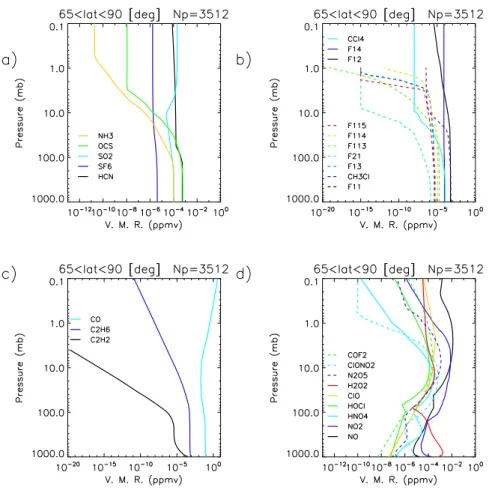
Gases for which there was much less global data at the time have been assigned constant tropospheric profiles, i.e., HCN, NH3, SO2, OCS, SF6, and the less abundant

halocarbons. The uncertainties in the profiles for these gases is therefore high. Finally

10

for CO₂, the profile is also the same for all five atmospheres as its variability was not believed to be significant compared to MIPAS requirements (see next section). Essen-tially, the CO2 profile was based on the estimated surface value for 2000 with a five

year time lag for the stratosphere and a modified profile above 80 km consistent with rocket soundings and the ATMOS results ofRinsland et al.(1992). Typical reference

15

profiles for CO2 and the operational species for MIPAS are shown in successive

fig-ures. Figure 1 therefore shows the standard atmosphere profiles for mid-latitudes for all remaining species (except N2 and O2) as examples of the standard atmosphere

profiles.

3.3 IG2 seasonal climatology

20

Although the standard atmospheres provide a good basic set of reference profiles, a zonal mean climatology is a more powerful means of encapsulating a greater range of atmospheric states in a regular manner whilst retaining a simple representation. In the case of MIPAS, this need for a simple climatology was driven by constraints imposed by the desire to constrain auxiliary data changes in the operational processor. This

25

had the beneficial impact of retaining a well-defined set of profiles for initial guess and contaminant profiles at the expense of less accuracy for contaminant profiles for a particular retrieval at a given location and time. The IG2 climatology developed in

(13)

ACPD

Printer-friendly Version Interactive Discussion this study represents the seasonal average atmosphere through a four season, six

latitude band set of states. The four seasons are centred on January, April, July and October. The six latitude bands are ±(90–65◦), ±(65–20◦), and ±(20–0◦). A common altitude grid of 0–120 km is employed for the seasonal climatologies as for the five standard atmospheres. The current version of the IG2 seasonal climatology is V4.0

5

and is the version used here for comparison to the operational MIPAS data. The IG2 data are downloadable as part of the auxiliary data for the MIPAS processing but are also available from the lead author of this paper.

In contrast to the standard atmospheres, the regular grid of the climatology allowed for and required a more automated processing. Therefore, the IG2 climatologies were

10

based on five sets of climatological data: the URAP data sets, the MOZART and SLIM-CAT models, the ECMWF analysis and the CIRA climatology. Where no appropriate data sets are available, the IG2 climatology defaults to the most recent standard at-mospheres, in this case the V3.1 data. An input grid was defined mapping each of the 24 IG2 conditions to one of the standard atmospheres. A priority order of data

15

utilisation was employed with defined ranges of validity for each of the input data sets with essentially the troposphere for MOZART and ECMWF H₂O data and the URAP data and SLIMCAT model data for the stratosphere; the URAP data has priority in the stratosphere.

One of the major updates to the IG2 climatology compared to the standard

atmo-20

spheres concerns carbon dioxide. Since the MIPAS pressure/temperature retrieval depends on knowledge of the CO2 mixing ratio, knowledge of this gas was felt to be

particularly important. Therefore, a dynamic climatology was developed compared to the standard CO2representation to account for trends in the mixing ratios. Clearly, the

concentrations of greenhouse gases in the climatologies need continuous updates due

25

to trends in their concentrations. However, it is also the case that for carbon dioxide there is some horizontal and vertical structure to the concentrations in the troposphere and stratosphere due to the combined effects of source distributions, the seasonal cy-cles in CO₂due to vegetative uptake, and the nature of transport into the stratosphere

(14)

ACPD

Printer-friendly Version Interactive Discussion with a slow transport of air to the poles. The IG2 V4.0 CO₂seasonal IG2 climatology

in-cludes these effects. The process starts with ground-based and aircraft measurements from the Globalview data set, which are advected into the stratosphere according to age of air relationships as a function of N₂O (Andrews et al.,1999); N₂O values in the stratosphere have been derived using compact relationships derived from ATMOS data

5

(Michelsen et al.,1998) because comparisons with equivalent relationships for CLAES data showed a clear bias in equatorial latitudes, presumably resulting from the residual effects of Mt. Pinatubo aerosol on the retrievals.

The efficacy of the age of air process is illustrated in Fig. 2 where tropical retrievals of CFC-12 from MIPAS data for July 2003, performed off-line using the OPERA scheme

10

at Leicester (Moore et al.,2006), are compared to V3 data from the ATMOS instrument updated for tropospheric trends (Cunnold et al.,2002). The agreement is very good as might be expected in the tropics where the age of air is younger than in the poles. The IG2 and tropical standard atmosphere are biassed high due to the Pinatubo effect on CLAES data. Uncertainty in the age of air will increase towards the poles but variations

15

in CO2should be close to the expected one sigma of 2 ppmv. To be conservative above

25 km, where the age of air becomes more uncertain, constant values are assumed for CO2due to the tropospheric source as represented at 25 km and only a small methane

oxidation term changes the vertical profile in the upper stratosphere. Above 80 km, upper atmosphere CO₂has been further modified to followLopez Puertas et al.(2000).

20

The atmosphere is updated on an annual basis using the latest CO2 Globalview data

sets.

Figure3shows the final V4.0 latitude dependent profiles produced for the 2003 an-nual average. On a full scale (left hand plot), there is clearly little variation of CO2 in

the troposphere and stratosphere. However, a finer scale (right hand plot) highlights

25

the structure present in the CO₂profiles, particularly in the troposphere but also in the vicinity of the tropopause. In the lower troposphere, there is a clear difference between the polluted northern hemisphere and the cleaner southern hemisphere. There is also considerable variability in the upper troposphere with potential for strong gradients into

(15)

ACPD

Printer-friendly Version Interactive Discussion the lower stratosphere. In the northern hemisphere this gradient may be particularly

strong because of the strong tropospheric seasonal cycle and anthropogenic inputs coupled to a long age of air for the lower stratospheric layers overlying the tropo-sphere. Differing values in the stratosphere reflect age of air variations with latitude as expected.

5

Similarly it will be important in the future to re-visit the MIPAS reference atmospheres for all tropospheric species to consider in more detail the variability of key species. Currently the IG2 seasonal climatology already contains variations, for example of tro-pospheric ozone. Nonetheless, scrutiny of the climatologies and updates for the range of satellite data available will provide insight into the climatological representation.

10

4 Comparisons with MIPAS operational geophysical products

The seven operational MIPAS products are profiles of pressure/temperature, H2O, O3,

HNO3, CH4, N2O and NO2 retrieved along an orbit-track,. As for the validation papers

in this MIPAS special issue, the aim of this study is to describe the chief characteristics of V4.61/V4.62 of the MIPAS operational product. The architecture of the operational

15

retrieval and optimised forward model, and the strategy for its implementation, are described in detail inRaspollini et al.(2006). Briefly, the retrieval is based on a global, non-linear least-squares fit of each entire limb sequence of spectra, with products being retrieved sequentially in the order in which they are listed above. The retrievals are performed in optimised microwindows extracted from calibrated, geo-located and cloud

20

flagged level 1b spectra and utilise a dedicated spectroscopic database. Estimated errors for the products are described in Raspollini et al. (2006) and can be found in more detail athttp://www-atm.atm.ox.ac.uk/group/mipas/err/.

(16)

ACPD

Printer-friendly Version Interactive Discussion 4.1 Cloud flagging

Cloud flagging is of some importance for MIPAS data quality. In MIPAS, cloud flagging is implemented in the operational processor, as described inSpang et al.(2004), using pairs of microwindows in the MIPAS spectral channels A, B and D in order of priority. The band A pair of microwindows is therefore of the highest priority and is used to flag

5

the majority of MIPAS data as cloudy or non-cloudy; its use depends only on the validity of the MIPAS A spectral data recorded for any limb observation (or sweep). The cloud index for channel A (CI-A) is defined as the ratio of the signals in two designated cloud microwindows (MIPAS band A), 788.2 to 799.25 cm−1 and 832.3 to 834.4 cm−1, such that values below a threshold value are used to indentify particularly cloudy spectra

10

which are not used in the geophysical product retrievals. The V4.61/V.62 processor employed a value of 1.8 for the CI-A threshold. In fact optically thinner clouds (cloud index greater than 1.8) may also cause residual errors in the trace gas retrievals and the definition of threshold is dependent to some extent on the degree of systematic error that can be tolerated for a given application. For example,Waterfall et al.(2004)

15

with respect to all gases andGlatthor et al.(2006) with respect to ozone have indicated values of 2.2 and 4.0 respectively for more rigorous flagging than the current opera-tional processing. The comparisons to reference atmospheres in this study afford some evidence for better definition of the CI-A threshold, in particular for CH₄ and N₂O. All MIPAS geophysical data examined in this study are only utilised if a valid CI-A cloud

20

flag can be computed and its value examined. 4.2 Results for MIPAS operational data

In this study, each of the MIPAS geophysical products have been compared to the MI-PAS reference atmospheres on a monthly basis for each month in 2003. However most of the results in a climatological sense are consistent across the year and hence the

25

plots in Figs.4to 18are based on the month of July 2003, except for those for O₃. Each of the main plots is composed of two panels. In the left hand panel, labelled (a), the

(17)

ACPD

Printer-friendly Version Interactive Discussion objective is to examine mean profiles and compare the variability of MIPAS data with

that expected. Individual MIPAS data points are represented by small crosses, with black indicating cloud-free measurements, and red crosses indicating measurements with a CI-A of less than 2.5 (see comments below for CH₄ and N₂O). All data plots plotted are those with a valid CI-A flag and with valid convergence criteria. Ranges for

5

the plots are chosen so as to show the chief features of the profiles and not all MIPAS points may appear on them. In particular, it was observed in this study that all MIPAS trace gas products show values of 10−10occasionally, these values being the result of retrieval instabilities (see Fig.17for NO2). Mean profiles from the MIPAS data are

rep-resented by the larger green (mean of data with CI-A >2.5) and red (all data) crosses.

10

The reference atmosphere profiles plotted are the corresponding IG2 climatologies (or-ange line) together with the associated three-sigma values (dotted or(or-ange lines) and the appropriate standard atmosphere with maximum and minimum thresholds (blue lines). Since the standard atmospheres are only derived for five atmospheric states, one would expect that these would show the larger discrepancies from the observed

15

data. The right hand panel plots illustrate the variability in a different manner, i.e. via a calculated sigma for the various data sources: one-sigma values from the IG2 cli-matologies (light orange dotted lines) compared to sigma uncertainties in the standard atmospheres ((max-min)/6: the dark orange dashed lines) and the standard deviation of MIPAS measurements for a given month for cloud-free scenes (green diamonds)

20

and cloud-flagged scenes (black asterisks). Sigmas derived from maximum/minimum profiles will not necessarily agree with the IG2 sigmas and the latter should be a better estimate. An upper limit of 0.01 mb is used in the plots based on the upper altitude range of MIPAS data.

Temperature data shown in Fig.4indicate the general agreement with MIPAS data

25

in mid-latitudes and tropics. Monthly mean data in 2003 typically agree very well away from the polar regions. For temperature, the standard deviations in the IG2 atmo-spheres are derived from the standard atmoatmo-spheres directly hence only one variability line on the plots. The agreement shown is also typical with MIPAS data tending to

(18)

ACPD

Printer-friendly Version Interactive Discussion show a variability of approximately 3 K in the middle stratosphere, away from the winter

pole, whereas the reference sigmas tend to vary between 3 and 5 K. In the polar re-gions, there are larger discrepancies between MIPAS data and the IG2 climatology in either the lower stratosphere, e.g. in the Antarctic winter, or in the upper stratosphere in the summer pole. However, there is considerable variability in temperatures in this

5

region and further study is required to investigate whether the effects are interannual variability or problems with either the instrument data or the reference atmospheres.

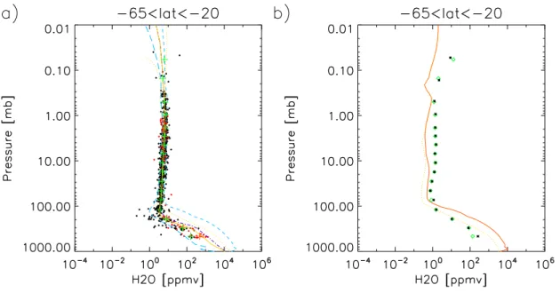
Figures 5 and 6 show comparisons for H₂O which essentially cover two main regimes, the dry stratosphere and the increasingly moist troposphere. In the tropo-sphere, mean MIPAS profiles and reference atmosphere profiles agree well in shape

10

but the mean MIPAS data (cloud free) are lower than both reference atmosphere pro-files, a result which is typical of comparisons for 2003. This apparent discrepancy is likely to be a consequence of the fact that the reference atmospheres are expected to be typical of all conditions whereas the MIPAS data are biassed towards thin cloud and clear sky. However, the estimated systematic uncertainty in MIPAS observations

15

is also large in this region and of the order of 30%. It is also noticeable that whilst there are considerable positive discrepancies in the cloudier flagged data (mean of all data greater than mean for CI-A <2.5), there are also a number of very low MIPAS data points particularly near the cold tropopause. Although there is a possibility of low H₂O mixing ratios, evidence from retrieval simulations suggest that the lowest MIPAS

20

values can arise from two sources: (a) limitations in the MIPAS operational proces-sor to retrieve accurately in this situation; (b) a tendency of the H2O retrieval to assign

anomalously low values at heights imemediately above unflagged clouds near the CI-A threshold. The dry constrained nature of stratospheric H2O, with values limited to a few

ppmv is evident in Fig.5 for the tropics. Mean values agree particularly well between

25

20 mb and 5 mb with the MIPAS mean data higher than the reference atmosphere data. At pressures of greater than 20 mb, some tendency towards an oscillating mean profile can be seen. Individual data points sit very well within the max/min profiles and stan-dard deviations are in reasonable agreement indicating random noise and atmospheric

(19)

ACPD

Printer-friendly Version Interactive Discussion variability of 10% or less 1 sigma; expected random errors vary between 5 and 10% in

the middle stratosphere. Similarly good comparisons are generally observed between MIPAS and the IG2 data in the southern hemisphere summer but the sigmas are larger for MIPAS data in the northern hemisphere winter.

For ozone, data from October 2003 illustrates the main features very well (Figs. 7

5

and8). In the tropical stratosphere, there is excellent agreement between mean MIPAS profiles and the reference atmosphere profiles, demonstrating the well-constrained and characterised stratospheric profile. As for H₂O in the stratosphere, climatological rep-resentations tend to do a good job of representing most of the stratospheric behaviour. Relative to MIPAS data, the minimum profile tends to be rather low but it is also

notice-10

able that the one sigma standard profiles tend to be smaller than the IG2 and MIPAS one sigma profiles. This implies that distributions are somewhat narrower than would be expected from maximum and minumum profiles as representing three sigma ex-tremes. In the southern polar spring, much better agreement between sigma profiles is obtained. The low ozone values for the mean profile and the data points are most

15

likely real with the neither reference atmosphere particularly capturing the lowness of the Antarctic ozone hole in this year. However, the IG2 data do a better job of capturing the variability represented by the individual MIPAS observations than do the standard atmosphere one sigmas. Both plots show high and low ozone values potentially as-sociated with CI-A less than 2.5 in the troposphere, with more variability clear in the

20

Northern high latitudes. Tropospheric concentrations from MIPAS are lower than the reference atmosphere profiles, particularly in equatorial regions and mid-latitudes (not shown).

Methane and nitrous oxide are dynamical tracers which are “well-mixed” in the tro-posphere with faster sinks in the stratosphere. Their observed distributions therefore

25

provide a good test of data quality. Figures9 and 10 show results for CH₄ in south-ern mid-latitudes and northsouth-ern polar summer respectively. The agreement betwen the MIPAS data and the reference atmosphere is generally very good in both mean and variability compared to standard max/min and IG2 sigma. In Fig.9, at altitudes near

(20)

ACPD

Printer-friendly Version Interactive Discussion 1 mb, there is a lower CH₄ concentration probably due to descent since it becomes

larger near the southern pole. Near 10.0 mb, an increased variability is observed which is under investigation. In polar summer, the agreement between the mean data sets is excellent for the entire profile. The IG2 sigmas appear to be considerably overesti-mated as do the max/min profiles. In the polar summer mean plot, there is a noticeable

5

set of red points which deviate considerably from the expected tropospheric concentra-tions in both a negative and positive sense. The distribuconcentra-tions of CH₄are well known in the troposphere with small variances of less than 10% expected as can be seen from the reference atmosphere variability profiles. Here it is the MIPAS data that are in error due to residual clouds effects with somewhat persistent polar cirrus likely to be present.

10

Similar effects can be seen for the southern mid-latitudes plots although not as clearly. The red points at pressures of less than 10 mb are not clouds but are due to noise in the CI-A test at 2.5; recall that the operational processor flags the data at 1.8 which is a lower threshold.

The cloud effects are examined further in Fig. 11where the average and standard

15

deviation of MIPAS data have been computed as a function of CI-A (bins of 0.5 in CI-A) for each hemisphere at latitudes of less than 50◦_{and pressures greater than}

150 mb. For low CI-A values, indicating thicker clouds/aerosol particle concentrations, it is clear that both the mean and the standard deviations of the measurements increase considerably for CI-A less than 3.0 or even 3.5 (northern hemisphere plot). Using

20

this test, it is not possible to be exact about the expected behaviour since CH4in the

upper troposphere will deviate slightly from constant volume mixing ratio if only due to transport and mixing of tropospheric and stratospheric air. In addition, there is a hemispheric gradient of approximately 0.1 ppmv as well as possible variability due to fast transport of surface concentrations. So for example, the gradient observed for the

25

southern hemisphere with CI-A may be entirely due to the gradient of CH₄with height rather than particle effects on the retrieval. Expected values of tropospheric surface CH4 have been estimated from values observed by the AGAGE network (Prinn et al.,

2000;Cunnold et al.,2002) as 1.829 and 1.732 ppbv for the northern hemisphere and 9991

(21)

ACPD

Printer-friendly Version Interactive Discussion southern hemispheres respectively. Applying a threshold of CI-A of 3.5 would then

suggest that more stringent cloud flagging results in “clear sky” CH4values which are

less than 10% high and that the random error in the retrieval (noise) is of the order of 10% also. These error estimates are broadly consistent with those expected from the MIPAS estimated error budget for the upper troposphere, with the limiting factor being

5

temperature uncertainties.

Similar evaluations have been performed for nitrous oxide. The comparisons here are shown on the usual altitude scale for southern mid-latitudes and an expanded altitude scale plot for the tropics to illustrate effects on N2O in more detail. In Fig. 13,

the mean profile and standard deviations are in excellent agreement in the stratosphere

10

with a considerably lower MIPAS mean profile in the upper stratosphere. Again there is an effect of increased variability at approximately 10 mb as for CH4. The results

shown in Fig.12illustrate how the reference atmosphere data encapsulate both mean and standard deviations rather well in the lower stratosphere. However from 100 mb and below, higher deviations can be seen which are most likely cloud effects and also

15

the data are perhaps more variable indicating that single profile noise is higher than expected atmospheric variability. Figure 14shows plots for N₂O mean concentrations versus CI-A, as for CH4. Similar results are found, with high sensitivity to CI-A in

mean and standard deviation for CI less than 2.5. For higher CI-A thresholds, residual uncertainties might be just over 10% systematic and 10% random error, reducing a

20

little as the CI-A threshold is increased. It is possible that the actual total systematic error in MIPAS data from non-cloud sources is less than 5% but it is not possible to be definitive about this.

For the remaining two gases, nitric acid and nitrogen dioxide, it is not possible to undertake the same types of cloud tests. Figures15 and16 show data for nitric acid

25

for northern polar summer and for southern mid-latitudes respectively representing contrasting views of nitric acid. Considering the former first, excellent agreement is seen in profile shape and magnitude between 100 mb and 7 mb. At higher altitudes, the random error increases considerably but there is also a significant difference in the

(22)

ACPD

Printer-friendly Version Interactive Discussion nitric acid data. At lower altitudes, cloud effects become significant and the mean HNO3

profile, even for the green crosses, is considerably larger than the reference state in the upper troposphere at altitudes below a pressure of 150 mb. It is not possible in this study to say whether this is due to cloud effects on retrievals or interactions in the atmosphere between cloud particles and nitric acid.

5

Figure17shows nitrogen dioxide data comparisons and highlights some of the cur-rent issues with the operational NO₂ product. The MIPAS data for NO₂ are retrieved in a restricted altitude range within which the mean and sigma values for NO2are well

characterised in the reference atmospheres and match well with MIPAS data. This is particularly true of the standard deviations in all latitudes and altitudes except for the

10

southern polar regions (not shown). In the mean profile, the comparisons are very good except at the high altitudes where the diurnal variability of NO2 complicates

interpre-tation of the plots. However, clear separation can be seen in the southern midlatitude plot for regions above 1 mb, with part of the data set clearly converging near the IG2 climatological profiles, and part of the data set retrieving significantly lower

concentra-15

tions closer to the nighttime standard atmosphere. Erroneous values of 10−10are also present in the operation product, and shown here. These are believed to be instabil-ities in the operational retrieval processor within the limits of convergence allowed for computing time.

5 Summary

20

In this paper, the MIPAS reference atmospheres have been introduced and descriptions given of the current five standard atmospheres (V3.1) and the IG2 seasonal climatology (V4.0). These atmospheres include not only mean concentrations for 36 species from 0 to 120 km, as well as pressure and temperature, but also estimates of variability. For the standard atmospheres, the aim was to capture the maximum/minimum values

25

of each species at each altitude, i.e., the extreme values,in order to assess the full range of possible atmospheric distributions within practical constraints. One sigma

(23)

ACPD

Printer-friendly Version Interactive Discussion standard deviations can be estimated from the maximum/minimum profiles, assuming

Gaussian statistics but this clearly is not a good assumption for many trace species. For sigma values, it is probably better to use the IG2 data for which these values have been calculated explicitly. A significant aspect of the IG2 climatology is the addition of a dynamic, yearly dependent update through the development of a time varying CO2

5

climatology. For other “well-mixed” gases in the troposphere, changes were not found to be significant for most species but HCFC-22, CFC-113 and CFC-115 clearly require further updates.

The MIPAS reference atmospheres have been compared to MIPAS observations for 2003 (full spectral resolution mode) and are revealing. It is found that the MIPAS data

10

agree very well with the reference atmospheres in mean behaviour at most altitudes, verifying the consistency of the reference states and the independent MIPAS data. Agreements are particularly good for the middle stratosphere data. Discrepancies due to clouds and noise have been noted at the upper and lower limits of the MIPAS retrieval range. For methane and nitrous oxide, it has been demonstrated that cloud influences

15

on the retrieval are important, and are presumably so for other species. The results presented here suggest that for the highest accuracy, MIPAS data should be filtered with cloud index values of 2.5 for N2O and 3.5 for CH4. Once such filtering has been

performed, the MIPAS data for these species appear to be accurate to within 10% in the upper troposphere. The presence of data with values of 10−10 _{has also been}

20

identified in all the products despite the use of MIPAS convergence flags. It is believed that these arise from retrieval instabilities. There are also some regions where MIPAS data are not in good agreement with the mean climatological profiles particularly in polar regions in the lower stratosphere and troposphere. These will be investigated further. The results presented here illustrate the significant utility of comparisons of

25

observed data with reference climatological atmospheric states. The use of cloud index data in combination with MIPAS data is recommended for studies of the polar winter stratosphere and the upper troposphere/lower stratosphere.

(24)

ACPD

AO-357, CUTLSOM), the MIPAS QWG for many valuable comments and the NOAA for provi-sion of the Globalview data set.

References

Anderson, G. P., Chetwynd,J. H.,Clough, S. A. , Shettle E. P., Kneizys F. X.,: AFGL Atmospheric Constituent Profiles (0–120 km), AFGL-TR-86-0110, Environ. Res. Papers No. 954 (1986),

5

ADA175173. 9975,9981

Andrews, A. E., Boering, K. A., Daube, B. C., Wofsy, S. C., Hintsa, E. J., Weinstock, E. M., and Bui, T. P.: Empirical age spectra from observations of stratospheric CO₂: Mean ages, vertical ascent rates, and dispersion in the lower tropical stratosphere, J. Geophys. Res., 104, 26 581–26 595, 1999. 9985

10

Brasseur, G. P., Hauglustaine, D. A., Walters, S., Rasch, P. J., M ¨uller, J.-F., Granier, C., and Tie, X. X.: MOZART, a global chemical transport model for ozone and related chemical tracers, 1, Model description, J. Geophys. Res., 103(D1), 28 265–28 289, 1998. 9980

Chiou, E. W., McCormick, M. P., Chu, W. P., et al.: Global water-vapor distributions in the stratosphere and upper troposphere derived from 5.5 years of SAGE II observations (1986–

15

1991), J. Geophys. Res., 102, 19 105–19 118, 1997. 9975,9978

Chipperfield, M. P.: Multiannual Simulations with a Three-Dimensional Chemical Transport Model, J. Geophys. Res., 104, 1781–1805, 1999. 9980

COSPAR International Reference Atmosphere 1986, Part II: Middle Atmosphere Models, edited by: Rees, D., Barnett, J. J., Labitzke, K., Adv. Space Res., 10(12), 1990.9975,9978,9982

20

Cunnold, D. M., Steele, L. P., Fraser, P. J., Simmonds, P. G., Prinn, R. G., Weiss, R. F., Porter, L. W., Langenfelds, R. L., Wang, H. J., Emmons, L., Tie, X. X., and Dlugokencky, E. J.: In situ measurements of atmospheric methane at GAGE/AGAGE sites during 1985–2000 and resulting source inferences, J. Geophys. Res., 107(D14), 4225, doi:10.1029/2001JD001226, 2002. 9985,9991

25

Echle, G., Oelhalf, H., and Wegner, A.: Measurements of atmospheric parameters with MIPAS, Final Report, ESA Contract 9597/91/NL/SF, 1992.9975,9981,9982

Fischer, H. and Oelhaf, H.: Remote sensing of vertical profiles of atmospheric trace con-stituents with MIPAS limb-emission spectrometers, Appl. Opt., 35, 2787–2796, 1996.9976

Fischer, H., Blom, C. E., Oelhaf, H., Carli., B, Carlotti, M., Delbouille, L, Ehhalt, D., Flaud,

30

(25)

ACPD

J.-M., Isaksen, I., Lopez-Puertas, M., McElroy, C. T., and Zander, R.: ENVISAT, MIPAS An instrument for ATmospheric Chemistry and Climate Research , editors C. Readings and R. A. Harris, ESA Publications Division, ESTEC, P. O. BOx 299, 2200, AG Noordwijk, The Netherlands, SP-1229, 2000.9976

Fortuin, J. P. F. and Kelder, H.: An ozone climatology based on ozonesonde and satellite

mea-5

surements, J. Geophy. Res., 103(D24), 31 709-31 734, 1998 9975,9978,9982

Greenhough, J., Remedios, J. J., Sembhi, H., and Kramer, L. J.: Towards cloud detection and cloud frequency distributions from MIPAS infra-red observations, Adv. Space Res. 36, 800–806, 2005.

Glatthor, N., von Clarmann, T., Fischer, H., Funke, B., Gil-Lpez, S., Grabowski, U., Hpfner, M.,

10

Kellmann, S., Linden, A., L ´opez-Puertas, M., Mengistu Tsidu G., Milz, M., Steck, T., Stiller, G. P., and Wang, D.-Y.: Retrieval of stratospheric ozone profiles from MIPAS/ENVISAT limb emission spectra: a sensitivity study, Atmos. Chem. Phys., 6(10), 2767–2781, 2006 9987

GLOBALVIEW-CO 2: Cooperative Atmospheric Data Integration Project - Carbon Dioxide. CD-ROM, NOAA GMD, Boulder, Colorado [Also available on Internet via anonymous FTP to

15

ftp.cmdl.noaa.gov, Path: ccg/co2/GLOBALVIEW], 2006 9979

Hauglustaine, D. A., Brasseur, G. P., Walters, S., Rasch, P. J., M ¨uller, J.-F., Emmons, L. K., and Carroll, M. A.: MOZART, a global chemical transport model for ozone and evaluation, J. Geophys. Res., 28 291–28 335, 1998a.9980

Intergovernmental Panel on Climate Change (IPCC): Climate Change 2001: The Scientific

Ba-20

sis, Contribution ofWorking Group I to the Third Assessment Report of the Intergovernmental Panel on Climate Change, edited by: Houghton, J. T., Ping, Y., Griggs, D. J., et al., pp.944, Cambridge University Press, UK, 2001.9999

Intergovernmental Panel on Climate Change (IPCC) Special Report on Safeguarding the Ozone Layer and the Global Climate System Issues related to Hydrofluorocarbons and

Per-25

fluorocarbons, edited by: Metz, B., Kuijpers, L., Solomon, S., et al., pp.478, Cambridge University Press, UK, 2005 9999

Kleinert, A., Aubertin, G., Perron, G., Birk, M., Wagner, G., Hase, F., Nett, H., and Poulin, R.: MIPAS Level 1B Algorithms Overview: Operational Processing And Characterization, Atmos. Chem. Phys., 7, 1395–1406, 2007,

30

http://www.atmos-chem-phys.net/7/1395/2007/. 9977

Lopez Puertas, M., Lopez Valverde, M. A., Garcia, R. R., and Roble, R. G.: A review of CO and CO2 abundances in the mesosphere and lower thermosphere.In Atmospheric Science

(26)

ACPD

Across the Stratopause, edited by: Siskind, D. E., Eckermann, S. D., and Summers, M. E., Meteor. Monogr., 123, 83–100, 2000. 9985

Michelsen, H., Manney, G. L., Gunson, M. R., Zander, R.: Correlations of stratospheric abun-dances of CH4 and N2O derived from ATMOS measurements, Geophys. Res. Lett., 25, 2777–2780, 1998. 9985

5

Moore, D. P., Waterfall, A. M., Remedios, J. J.: The potential for radiometri retrievals of halocar-bon concentrations from the MIPAS-E instrument, Adv. Space Res., 37, 2238–2246, 2006.

9985

O’Doherty, S., Cunnold, D., Sturrock, G. A., Ryall, D., Derwent, R. G., Wang, H. J., Simmonds, P., Fraser, P. J., Weiss, R. F., Salameh, P., Miller, B. R., and Prinn, R. G.: In-situ

chloro-10

form measurements at AGAGE atmospheric research stations from 1994–1998, J. Geophys. Res., 106, 20 429–20 444, 2001. 9999

Prinn, R. G., Cunnold, D. M., Rasmussen, R., Simmonds, P. G., Alyea, F. N., Crawford, A., Fraser, P. J., and Rosen, R.: Atmospheric emissions and trends of nitrous oxide deduced from ten yearsof ALE-GAGE data, J. Geophys. Res., 95, 18 369–18 385, 1990.

15

Prinn, R. G., Weiss, R. F., Fraser, P. J., Simmonds, P. G., Cunnold, D. M., Alyea, F. N., O’Doherty, S., Salameh, P., Miller, B. R., Huang, J., Wang, R. H. J., Hartley, D. E., Harth, C., Steele, L. P., Sturrock, G., Midgley, P. M., and McCulloch, A.: A History of Chemically and Radiatively Important Gases in Air deduced from ALE/GAGE/AGAGE, J. Geophys. Res., 105, 17 751–17 792, 2000. 9979,9991

20

Randel, W. J., Wu, F., Russell III, J. M., and Waters, J. W.: Space-time patterns of trends in stratospheric constituents dericed from UARS observations, J. Geophys. Res., 104, 3711– 3727,19999979,9982

Raspollini, P., Belotti, C., Burgess, A., Carli, B., Carlotti, M., Ceccherini, S., Dinelli, B. M., Dudhia, A., Flaud, J.-M., Funke, B., Hoepfner, M., Lopez-Puertas, M., Payne, V., Piccolo,

25

C., Remedios, J. J., Ridolfi, M., and Spang, R.: MIPAS level 2 operational analysis, Atmos. Chem. Phys., 6, 5605–5630, 2006,

http://www.atmos-chem-phys.net/6/5605/2006/. 9977,9986

Rinsland, C. P., Gunson, M. R. , Zander, R., and Lopez-Puertas, M.: Middle and Upper At-mosphere Pressure-Temperature Profiles and the Abundances of CO2 and CO in the Upper

30

Atmosphere from ATMOS/Spacelab 3 Observations J. Geophys. Res., 97, 20 479–20 495, 1992 9983

Roche, A. E., Kumer, J. B., Nightingale, R. W., Mergenthaler, J. L., Ely, G. A., Bailey, P. L.,

(27)

ACPD

Massie, S. T., Gille, J. C., Edwards, D. P., Gunson, M. R., Abrams, M. C., Toon, G. C., Webster, C. R., Traub, W. A., Jucks, K. W., Johnson, D. G., Murcray, D. G., Murcray, F. H., Goldman, A., and Zipf, E. C.: Validation of CH4 and N2O measurements by the Cryogenic limb array Etalon spectrometer instrument on Upper Atmosphere Research Satellite, J. Geo-phys. Res., 101, 9679–9710, 1996.

5

Swinbank, R. and O’Neill, A.: A Stratosphere-Troposphere Data Assimilation System, Mon. Wea. Rev., 122, 686-702, 19949980

Spang, R., Remedios, J. J., Kramer, L. J., Poole, L. R., Fromm, M. D., Mller, M., Baumgarten, G., and Konopka, P.: Polar stratospheric cloud observations by MIPAS on ENVISAT: detec-tion method, validadetec-tion and analysis of the northern hemisphere winter 2002/2003’, Atmos.

10

Chem. and Phys., 5, 679–692, 2005.9977

Spang R., Remedios, J. J., and Barkley M. P.: Colour indices for the detection and differentiation of cloud types in infra-red limb emission spectra, Adv. Space Res., 33(7), 1041–1047, 2004.

9987

U.S. Standard Atmosphere, 1976, NOAA-S/T 76-1562, 1976. 9975

15

Wang, H. J., Cunnold, D. M., Froidevaux, L., and Russell III, J. M.: A reference model for middle atmosphere ozone in 1992/1993, J. Geophys. Res. 104, 21 629–21 643, 1999. 9979

Waterfall, A. M., Remedios, J. J., Spang, R., and Sembhi, H.: Validation of the MIPAS Level 2 products using reference atmospheres, Proceedings of the ACVE-2 workshop, 2004. 9987

(28)

ACPD

Printer-friendly Version Interactive Discussion Table 1. Comparison of MIPAS standard atmosphere mean trospheric values for well-mixed

gases compared to IPCC estimates (IPCC,2001, 2005). Values for CH₃Cl are derived from Mace Head(a) and Cape Grim(b) observations (O’Doherty et al.,2001).

Gas MIPAS reference atmosphere (pptv) 2000 estimate (pptv) 2003 estimate

CO₂(ppmv) 369 367 375 CH₄(ppmv) 1.760 1.745 1.732 N₂O (ppmv) 3.17 3.14 3.18 CFC-11 265 268 256 CFC-12 545 533 538 HCFC-22 140 132 157 CFC-113 19 84 80 CFC-114 12 15 17 CFC-115 4 7 17 CH₃Cl 700 – 532a, 510b CCl₄ 108 102 96 9999

(29)

ACPD

Printer-friendly Version Interactive Discussion Fig. 1. Equatorial profiles of all species covered by the IG2 climatologies, excluding CO₂, N₂O,

(30)

ACPD

Printer-friendly Version Interactive Discussion Fig. 2. Comparison of mean MIPAS CFC-12 offline retrievals(OPERA) for July 2003 with

AT-MOS data updated using age of air and tropospheric trends. The corresponding tropical IG2 profile for July and the tropical standard atmosphere are also shown.

(31)

ACPD

Printer-friendly Version Interactive Discussion Fig. 3. Left Panel: IG2 profiles for CO₂for all 6 latitude bands for 2003. Right Panel: Detail of

(32)

ACPD

Printer-friendly Version Interactive Discussion Fig. 4. Comparison of MIPAS and reference atmosphere temperature data for latitudes from

20 N to 65 N for July 2003: Left panel - Operational MIPAS data from July 2007 for “cloudy” data (CI-A <2.5 – red dots) and “clear-sky” data (CI-A >2.5 – black dots). Means for the cloudy data (large red crosses) and clear data (large green crosses) at each scan altitude are also shown. Plotted in blue are the standard atmosphere profile and associated maximum and minimum values (dashed lines) for this latitude band and period. Orange lines represent the IG2 climatologies with 1 sigma values (dashed) for this latitude band and period. Right panel -The standard deviation of the MIPAS values at each scan altitude are shown in green diamonds (clear sky data only) and black asterisks (all data including cloudy data). One sigma values for the IG2 climatologies are shown in light orange dotted lines, while an estimate of one sigma values for the standard atmospheres is shown by the dark orange dashed lines.

(33)