Autonomous & Adaptive Oceanographic Feature Tracking On Board
Autonomous Underwater Vehicles
by
Stephanie Marie Petillo
B.S., Aerospace Engineering, University of Maryland, College Park (2008) Submitted to the Joint Program in Applied Ocean Science & Engineering
in partial fulfillment of the requirements for the degree of Doctor of Philosophy in Oceanographic Engineering
at the
MASSACHUSETTS INSTITUTE OF TECHNOLOGY and the
WOODS HOLE OCEANOGRAPHIC INSTITUTION February 2015
©2015 Stephanie M. Petillo. All rights reserved.
e author hereby grants to MIT and WHOI permission to reproduce and to distribute publicly paper and electronic copies of this thesis document in whole or in part in any medium now known
or hereafter created.
Author . . . . Joint Program in Oceanography/Applied Ocean Science & Engineering
Massachusetts Institute of Technology & Woods Hole Oceanographic Institution November 21, 2014 Certified by . . . .
Henrik Schmidt Professor of Mechanical and Ocean Engineering Massachusetts Institute of Technology esis Supervisor Accepted by . . . .
Henrik Schmidt Chairman, Joint Committee for Applied Ocean Science & Engineering Massachusetts Institute of Technology Woods Hole Oceanographic Institution Accepted by . . . .
David E. Hardt Chairman, Committee for Graduate Students Massachusetts Institute of Technology
Autonomous & Adaptive Oceanographic Feature Tracking On Board Autonomous Underwater Vehicles
by
Stephanie Marie Petillo
Submitted to the MIT/WHOI Joint Program in Applied Ocean Science & Engineering on November 21, 2014, in partial fulfillment of the
requirements for the degree of
Doctor of Philosophy in Oceanographic Engineering
Abstract
e capabilities of autonomous underwater vehicles (AUVs) and their ability to perform tasks both au-tonomously and adaptively are rapidly improving, and the desire to quickly and efficiently sample the ocean environment as Earth’s climate changes and natural disasters occur has increased significantly in the last decade. As such, this thesis proposes to develop a method for single and multiple AUVs to collaborate au-tonomously underwater while auau-tonomously adapting their motion to changes in their local environments, allowing them to sample and track various features of interest with greater efficiency and synopticity than previously possible with preplanned AUV or ship-based surveys. is concept is demonstrated to work in field testing on multiple occasions: with a single AUV autonomously and adaptively tracking the depth range of a thermocline or acousticline, and with two AUVs coordinating their motion to collect a data set in which internal waves could be detected. is research is then taken to the next level by exploring the problem of adaptively and autonomously tracking spatiotemporally dynamic underwater fronts and plumes using indi-vidual and autonomously collaborating AUVs.
esis Supervisor: Henrik Schmidt
Title: Professor of Mechanical and Ocean Engineering Massachusetts Institute of Technology
Biography
Stephanie Petillo grew up in Sterling, VA, and Acton, MA, where she attended Acton-Boxborough Regional High School. Her extracurricular activities involved marching band, dancing, Science Olympiad Team, figure skating, Girl Scouts, working on house projects and motor vehicles, riding dirt bikes in her backyard, and learning languages. Stephanie earned her Bachelor of Science Degree in Aerospace Engineering with a minor in Italian Language and Culture from the University of Maryland in College Park, MD, in 2008. While there she was a Team Leader of the Near Space balloon payload project, a Squad Leader of the trombone and baritone horn section of the Mighty Sound of Maryland marching band, an Apartment Leader for the Italian Cluster in the Language House, and she figure skated and raced cars competitively. Stephanie spent her final two summers of college in Woods Hole, MA, as a Guest Student in the WHOI Autonomous Systems Lab working with and deploying underwater gliders in 2006 and as a student at the Sea Education Association conducting oceanographic research and sailing a tall ship across the Pacific Ocean during an SEA Summer Semester in 2007. ese experiences influenced her undergraduate research thesis entitled “Evaluation of the Coordinated Sampling Performance of Underwater Gliders in Strong and Variable Currents: A Simulated Case Study in the Chesapeake Bay” and convinced her to switch into oceanographic engineering for graduate school.
Stephanie entered the Massachusetts Institute of Technology/Woods Hole Oceanographic Institution Joint Graduate Program following college to study Oceanographic Engineering. Her Doctoral research, which comprises this thesis, has focused on using autonomous underwater vehicles (AUVs) to perform autonomous and environmentally adaptive sampling of the ocean environment, focusing on underwater feature detection and tracking for more efficient and synoptic data collection with AUVs. Stephanie has enjoyed being on and near the ocean, working with oceanographic vehicles and instrumentation, and seeing her complex un-derwater vehicle missions work out in the water, and she has had the great opportunity of participating in over a dozen research cruises since she first started working with underwater vehicles in college. roughout graduate school, Stephanie has continued her many hobbies and activities, adding hiking, farming, sailing, and woodworking to the list.
Acknowledgments
First of all I would like to thank my advisor, Prof. Henrik Schmidt, for making this thesis possible. He has not only provided me with the opportunity to follow my own path with my PhD research, but also has been very
trusting in allowing his grad students to get their hands dirty with AUV deployments on numerous research cruises. My cruise count has certainly topped 10 by now, which is more than I could have hoped for coming into the Joint Program. I can truly say I have had a great time working with Henrik and appreciate all the trips to Italy and other cruise and conference travel he has let me participate in right up until the end of my time here. ank you!
Second I would like to thank the rest of my thesis committee, Dr. Arjuna Balasuriya, Prof. Pierre Ler-musiaux, and Dr. Dana Yoerger, for all of their invaluable input to my research. anks to Arjuna for collaborating with me from the beginning of my time at MIT and for providing us with pizza those late nights in the lab doing last-minute SWAMSI payload wiring. anks to Pierre for vouching for me during quals and always bending over backwards to get me whatever models or data I needed. anks to Dana for all the great stories from AUV deployments and life and for many discussions on plume tracking. I would also like to thank Dr. Hanu Singh for chairing my defense and looking after my progress on the WHOI side of things from the beginning of my time in the Joint Program.
ank you to Dr. Mike Benjamin for writing and maintaining the IvP Helm, which has made the many virtual and field experiments in this thesis possible. I have also appreciated the many insightful discussion we have had, and I especially appreciate your letting me kidnap more than my fair share of your laptops for a year to run my virtual experiments.
I would also like to thank all the members of the LAMSS lab past and present: ank you Toby for fixing nearly any software problem we threw at you on cruise and in the office, and for completing our A-team for every cruise we were on together. ank you also for being my partner in crime on cruise, on travel, and in life. I could not have completed this research nearly as efficiently without you there to devise all sorts of work-arounds when I wanted extra features to make my virtual experiments easier to run. ank you to Erin and Sheida for being both great friends and lab mates and for teaching me that it is okay to not be the only woman in an engineering lab! anks Stephanie for always being excited about my research and hosting craft nights. om, thanks for being such a quick learner on cruise and generally a fun person to hang out with. You will be a good replacement for me. Geoff, thanks for always being helpful and taking care of anything we needed for the lab, and thanks for always griping along with me whenever someone was doing something dumb. Tom and Aurthur, thanks for always being positive and being an integral part of the lab. It is good to have the perspective of you Navy guys reminding us that the real world is out there. Nick, thanks for taking over my work with the MSEAS group so it will hopefully not all get shelved once I am done. Alon, it has been fun working with you and listening to all your crazy ideas, even if I miss your media references 75%
of the time! Ian and Kevin, thanks for all the fun and serious discussions in the lab when there was a lull in productivity. Kevin, thanks also for always answering my questions about how to jump through the academic and thesis hoops and for treating me like all the other guys in the lab (that is a good thing!). Don, thanks for our discussions that got me started on front tracking and environmental sampling behaviors. Ray and Costas, it was great sharing the lab with you. Hopefully our paths will cross again. It has been a pleasure working with you all.
ank you also to Pierre, Pat Haley, and Wayne Leslie in the MSEAS group for, again, bending over backwards to get me the models, code, and information I needed for my research.
anks to Bluefin Robotics (and especially the operations guys) for the AUV support on every cruise, letting me help with AUV and instrument deployments, and basically training me to service the AUVs so I could do it all myself.
anks to all the folks I have worked with at the Centre for Maritime Research and Experimentation (CMRE) in La Spezia, Italy, including David Hughes, Marco Mazzi, Francesco Baralli, Kim McCoy, and the OEX and Autonomy groups who made my thermocline tracking and Internal Wave Detection Experiments possible.
anks to Mike Incze, Scott Sideleau, and Don Eickstedt from NUWC Newport for supporting the Champlain ’09 experiment for my research.
To the WHOI APO and all those that have taught, supervised, and mentored me since I first came to WHOI as a Guest Student, thank you!
I would like to thank the following programs and sponsors for funding and supporting my research, tuition, and stipend:
• e MIT/WHOI Joint Program
• Government support under and awarded by DoD, Air Force Office of Scientific Research, NDSEG Fellowship, 32 CFR 168a
• e U.S. Office of Naval Research (ONR) GOATS ’11 11-1-0097) and GOATS ’14 (N00014-14-1-0214) projects
• e ONR TechSolutions Program Office (Lightweight NSW UUV program)—Technical Support
• e Naval Undersea Warfare Center (NUWC) Division, Newport (Code 25)—Technical Support and Logistics
Finally, I would like to thank all of my friends from the Joint Program and beyond that have been nothing but supportive throughout my time in grad school. In particular I am grateful to have Derya, Ankita, Kalina, and Heather as my engineering friends who suffered through quals and classes with me in our first few years. I also owe a huge thanks to my family, and in particular my parents, who have always encouraged me to follow my dreams and do what I want to do in life and school. Mom and Dad, you cultivated my love of engineering and science and have bent over backwards to help and be supportive wherever possible throughout school, thesis writing, and all of my extracurricular adventures, and I can’t thank you enough! I think this comic sums it up pretty well:
“Completely implausible? Yes. Nevertheless, worth keeping a can of shark repellent next to the bed.”
Contents
1 Introduction 15
1.1 Concepts/Approach . . . 16
1.2 esis Outline & Contributions . . . 17
2 Background 21 2.1 Autonomous Adaptive Sampling . . . 21
2.2 Advantages & Challenges . . . 22
2.2.1 AUVs in the real environment . . . 22
2.2.2 AUV Networks . . . 24
2.2.3 Environmentally Adaptive Autonomy & Autonomous Coordinated Control . . . . 24
2.2.4 Acoustic Communication . . . 25
2.2.5 Data Fusion . . . 26
2.3 AUV technologies . . . 27
2.3.1 Autonomy Middleware . . . 27
2.3.2 Acoustic Communications . . . 28
2.3.3 Sensors & Instrumentation . . . 28
2.3.4 AUV Types . . . 30
2.4 Spatiotemporal Scales of Ocean Features . . . 32
2.4.1 Synoptic Sampling vs. Spatiotemporal Aliasing . . . 34
2.4.2 AUV Types and Numbers Suited to Different Features’ Scales . . . 35
2.5 Literature . . . 37
3 ermocline Tracking: A Proof-of-Concept for Autonomous Adaptive Environmental
3.1 Introduction . . . 39
3.2 Background & Importance . . . 40
3.2.1 Science/Oceanography . . . 40
3.2.2 Technology/Engineering. . . 41
3.3 Goals & Motivation . . . 41
3.4 Literature . . . 42
3.5 AAEA & Feature Tracking: A Novel Approach . . . 43
3.5.1 Oceanographic Features . . . 43
3.5.2 Defining a Feature Based on Data . . . 43
3.5.3 AAEA Process . . . 44
3.5.4 Tracking . . . 44
3.6 Tracking the Marine ermocline . . . 44
3.6.1 ermocline Definition . . . 44
3.6.2 Algorithm: ermocline Bounds and Maximum . . . 45
3.6.3 Algorithm Implementation on AUVs: pEnvtGrad . . . 47
3.6.4 Virtual Experiments & Testing . . . 49
3.7 Field Experiments & Results . . . 49
3.7.1 MIT Topside Setup . . . 50
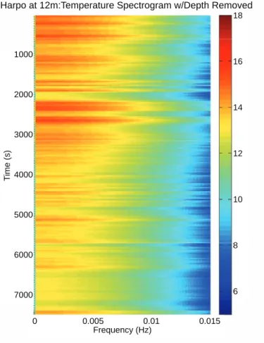
3.7.2 GLINT ’09—Acousticline Tracking . . . 51
3.7.3 GLINT ’09 Results . . . 52
3.7.4 Champlain ’09—ermocline Tracking . . . 54
3.7.5 Champlain ’09 Results . . . 54
3.7.6 GLINT ’10—ermocline Tracking for Internal Wave Detection . . . 56
3.7.7 GLINT ’10 Results . . . 57
3.8 Conclusion . . . 58
4 Internal Wave Detection Experiment 61 4.1 Introduction . . . 61
4.2 Goals . . . 61
4.3 Motivation . . . 62
4.4 Literature . . . 63
4.5.1 Hardware Platforms . . . 66
4.5.2 AUV Missions . . . 68
4.5.3 MOOS Processes and IvP Helm Autonomy Behaviors . . . 69
4.6 Data & Results. . . 72
4.6.1 Oceanographic Conditions . . . 73
4.6.2 Mission Execution. . . 73
4.7 Analysis . . . 77
4.8 Receiver Operating Characteristic Curves . . . 88
4.9 Conclusion . . . 89
4.10 Looking Ahead. . . 92
4.10.1 Further Data Analysis & Future Experiments . . . 92
4.10.2 Broader Applications . . . 93
5 Front Tracking 95 5.1 Introduction . . . 95
5.2 Goals . . . 96
5.3 Literature . . . 96
5.4 Novel Concepts & Approach . . . 97
5.5 2D & Multi-AUV Front Tracking . . . 101
5.5.1 Overview . . . 101
5.5.2 BHV_FrontTrackNoBdry (2D) . . . 103
5.5.3 BHV_FolloweLeader (Multi-AUV) . . . 104
5.6 3D Front Tracking . . . 106
5.6.1 BHV_FrontTrackHelix (3D) . . . 106
5.7 Virtual Experiments & Results . . . 109
5.7.1 MSEAS 4D Ocean Model Environment . . . 110
5.7.2 Preplanned Missions. . . 112
5.7.3 New Adaptive Missions . . . 113
5.7.4 Mission Configurations . . . 119
5.8 Analysis . . . 123
5.8.1 Performance Metrics . . . 123
5.9 Receiver Operating Characteristic Curves . . . 148
5.10 Conclusion . . . 149
6 Plume Tracking 155 6.1 Introduction . . . 155
6.2 Plumes . . . 156
6.2.1 Hydrothermal Vent Plumes . . . 156
6.2.2 Oil Spills . . . 157
6.2.3 Harmful Algal Blooms . . . 158
6.3 AUVs . . . 159
6.4 Plume Tracking Methods . . . 160
6.4.1 Related Literature . . . 161
6.4.2 Our Approach . . . 162
6.5 Conclusion . . . 165
7 Conclusion & Future Directions 167 7.1 Looking Ahead. . . 169
A MSEAS Integration 171 A.1 LAMSS-MSEAS Interface . . . 171
A.1.1 Virtual Experiment Environment . . . 171
A.1.2 Mission Simulation . . . 179
A.2 Topside Tools . . . 180
A.2.1 MSEAS Display . . . 180
A.2.2 CTD Display . . . 180
B Constructing a Distributed AUV Network for Underwater Plume-Tracking Operations 183 B.1 Introduction . . . 183
B.2 Spatiotemporal Aliasing Problem . . . 185
B.3 Advantages and Challenges of an AUV Network . . . 186
B.3.1 Working as a Team . . . 186
B.3.2 Autonomous Coordinated Control . . . 187
B.3.4 Data Fusion . . . 188
B.4 Adaptive Behavior Implementation . . . 189
B.4.1 ermocline Tracking as a Proof-of-Concept . . . 190
B.4.2 Plume Tracking . . . 191
B.5 Plume Simulation Environment . . . 193
B.5.1 Modeling a Plume . . . 194
B.5.2 Sampling a Plume . . . 195
B.5.3 Reconstructing a Plume from AUV Sample Points . . . 196
B.5.4 Results. . . 197
B.6 Forecasting Long Term Variations . . . 199
B.7 Looking Ahead. . . 201
Chapter 1
Introduction
“Telescopes and bathyscaphes and sonar probes of Scottish lakes, Tacoma Narrows bridge collapse explained with abstract phase-space maps, some x-ray slides, a music score, Minard’s Napoleonic war: the most exciting new frontier is charting what’s already here.”
http://xkcd.com/731/
Humans have used both sophisticated and simple instruments to help them understand and navigate the oceans for hundreds (if not thousands) of years. e taffrail log simply measured a ship’s speed through water. Soundings and sea floor materials were sampled from ships using a slug of lead on a string. e compass told sailors which direction they were heading, and the sextant helped them determine position. Not to mention
world maps were made from these measurements to further aid navigation. e past hundred years have seen many new oceanographic instruments developed as new materials became available and scientific interest in the ocean has greatly increased. Within the past fifty years, many of the original simple oceanographic technologies have been revisited and redesigned, and new technologies have emerged with the rapid and ongoing development of computer technology. Oceanographers and ocean engineers are always looking to improve ocean sampling technologies and systems, and are especially motivated by the fact that going to sea on a research vessel is expensive (tens of thousands of dollars per day). e expense limits time for data collection, often only allowing for one or two opportunities to collect a desired data set. If a data set is collected, but does not capture the feature or phenomenon the oceanographer requires, that is a costly misdirection of resources. at the limited data collected may still be of use to oceanographers researching this or some other subject is only a partial consolation.
Today, a number of groups are working on the problem of intelligent oceanographic sampling methods. One approach uses oceanographic data models and forecasts based on physics and/or previously collected data sets from a region to predict the location of an oceanographic feature of interest and attempt to sample an area accordingly with ship-based, moored, free-floating, or free-swimming instruments. Another approach is to use the developing technology of sensor-equipped unmanned underwater vehicles and/or unmanned surface vehicles running real-time intelligent autonomy algorithms to adapt the vehicle’s motion to changes in the environment, effectively seeking out and tracking an oceanographic feature of interest with very little or no previous knowledge of the ocean environment. Both of these methods result in adaptive sampling of the ocean environment. e focus of this thesis is the latter, aiming for more efficient and intelligent ocean sampling strategies by way of cutting-edge underwater vehicle technology and onboard autonomy systems.
1.1
Concepts/Approach
e goal of this work is to develop a system for the tracking of hydrographic features using autonomous underwater vehicles (AUVs). is tracking is done
• adaptively to account for the dynamic nature of hydrographic features,
• collaboratively between AUVs (and other marine platforms) to collect more complete data sets for feature detection, and
• autonomously such that the AUVs determine the spatiotemporal positions or boundaries of the fea-tures, to efficiently detect and track the features with as little human intervention as possible.
e motivation for this research stems from the need to sample the ocean in an increasingly low-cost, efficient, and intelligent manner such that scientists can predictively gather the data sets they need within a minimum of time aboard a research vessel. e use of AUVs with collaborative and adaptive autonomy also allows for measurements (environmental and otherwise) to be taken over a 3D area in space while still measuring time-dynamic properties. is gives a much greater probability of synoptic data coverage in the selected area of the ocean than using drifters, moored instruments, towed instruments, or AUVs without the ability to collaborate and adapt to changes in the environment.
e field of marine autonomy on unmanned underwater vehicles is advancing quickly, and the next step is to have the AUVs adapt their motion to the features of the underwater environment in real time, without guidance from an operator.
is thesis examines the methodology for performing autonomous and adaptive oceanographic feature tracking on board (solo and multiple) AUVs, addressing AUV autonomy, multi-AUV communication, and feature detection and tracking strategies. An emphasis is placed on the autonomous and adaptive coordinated sampling and tracking of four types of hydrographic features using AUVs: thermoclines, internal waves, and underwater fronts and plumes. e AUV autonomy system used here is comprised of the Mission Ori-ented Operating Suite (MOOS) and the Interval Programming (IvP) Helm [1,2]. e method of real-time underwater communication is assumed to be via acoustics, though other types of communication are consid-ered when the AUV is on the sea surface. e importance of synoptic sampling based on the characteristic spatiotemporal scales of ocean features is discussed, and the types of AUVs best suited for various scales of feature-tracking experiments are evaluated.
1.2
esis Outline & Contributions
e original research contributions of this thesis comprise part of Chapter2, all of Chapters3,4,5, &6, and the Appendices.
Chapter2: Background
is chapter provides the technical and oceanographic background for the thesis. It explains the concept of environmentally adaptive ocean sampling, some of the available AUV technologies, the challenges of working with AUVs in the ocean environment, and the concept of characteristic spatiotemporal scales of oceanographic features. is chapter also looks at past and current methods of oceanographic feature tracking from the literature to further motivate the work in this thesis.
Chapter3: ermocline Tracking: A Proof-of-Concept for Autonomous Adaptive Environ-mental Assessment and Feature Tracking
is chapter introduces the concept of Autonomous and Adaptive Environmental Assessment (AAEA) of oceanographic features using AUVs. is concept is then applied to thermocline tracking with AUVs as a proof-of-concept taken from theory to implementation. ermocline tracking results are given for multiple field experiments.
Chapter4: Internal Wave Detection Experiment
is chapter describes the Internal Wave Detection Experiment in the Tyrrhenian Sea in 2010. is ex-periment was designed to showcase the use of autonomous and adaptive thermocline tracking coupled with multiple autonomously coordinated AUVs to capture the signals of any passing internal waves. e results characterizing the detected internal waves are also presented.
Chapter5: Front Tracking
is chapter explores autonomously and adaptively detecting and tracking underwater fronts in detail. ese features are often significantly complex and dynamic in both horizontal space and time. 2D, 3D, and multi-AUV front tracking behaviors that have been developed for this work and tested in virtual experiments are described, and results from the tests in a simulated Multidisciplinary Simulation, Estimation, and Assimilation Systems (MSEAS) ocean model environment of the Mid-Atlantic Bight region are presented.
Chapter6: Plume Tracking
is chapter explores concepts and approaches for autonomously and adaptively detecting and tracking vari-ous types of underwater plumes.
Chapter7: Conclusion & Future Directions
e final chapter summarizes the contributions of this thesis and briefly explores the direction of future work on this subject.
AppendixA: MSEAS Integration
Appendix A details the integration of Massachusetts Institute of Technology (MIT) MSEAS ocean mod-els into the MIT LAMSS (Laboratory for Autonomous Marine Sensing Systems) AUV virtual experiment
environment and the associated GEOV (Google Earth interface for Ocean Vehicles) topside display. e MSEAS-LAMSS interface is described, as well as the interface for the MSEAS environmental display (over-lay) in Google Earth and the topside CTD display.
AppendixB: Constructing a Distributed AUV Network for Underwater Plume-Tracking Op-erations
AppendixBpresents original research conducted as an initial foray into a plume boundary parametrization and tracking method for AUVs.
Chapter 2
Background
is chapter provides the technical and oceanographic background and motivation for the research presented in the body of the thesis. is chapter is divided into five sections: an introduction to adaptive sampling, a description of some of the challenges of working with AUVs in the ocean environment, an explanation of some of the available AUV technologies, an explanation of the concept of characteristic spatiotemporal scales of oceanographic features, and a literature review motivating the need for autonomous and adaptive approaches to feature tracking using AUVs.
2.1
Autonomous Adaptive Sampling
e adaptive sampling methods that are applied in this thesis result in targeted observations of the ocean environment where a feature of interest is present. Adaptive sampling for this particular application is a two-step process that includes initially assessing (surveying and analyzing) the local environment to determine the presence of an oceanographic feature and subsequently tracking that feature over space and time to maintain
Portions of this chapter are ©2010 IEEE. Reprinted, with permission, from S. Petillo, A. Balasuriya, and H. Schmidt, “Autonomous Adaptive Environmental Assessment and Feature Tracking via Autonomous Underwater Vehicles,” Proceedings of OCEANS 2010 IEEE - Sydney. [3]
Portions of this chapter are ©2012 Stephanie Petillo et al. Reprinted, with permission, from S. Petillo, H. Schmidt, and A. Balasuriya, “Constructing a Distributed AUV Network for Underwater Plume-Tracking Operations,” International Journal of Distributed Sensor Networks: Special Issue on Distributed Mobile Sensor Networks for Hazardous Applications. [4]
Portions of this chapter are ©2010 IFAC. Reprinted, with permission, from S. Petillo and H. Schmidt, “Autonomous and Adaptive Plume Detection and Tracking with AUVs: Concepts, Methods, and Available Technology,” Proceedings of the 9th IFAC Conference on Manoeuvring and Control of Marine Craft. [5]
focused sampling in the region of study. e motivation behind adaptive sampling is to increase the efficiency of sampling and the synopticity of the collected data. is research focuses on the use of AUVs with onboard autonomy systems and environmental sensors to adaptively sample the ocean environment at and around features of interest using the aforementioned two-step process in real time. is results in a feedback loop involving environmental sensor readings, onboard data processing, and the autonomy system updating the desired motion of the AUV to adapt to and track the motion of a dynamic ocean feature to collect more data. is concept is sketched in Fig.2-1and applied in the body of this work.
Temperature [°C] D e p th [ m ] 0 20 40 60 14 18 22 28 Onboard Adaptive Feature Determination MOOS Middleware & IvP Helm Autonomy Determines Thermocline Depth Bounds
Adapts Yoyo Max / Min Depths to Thermocline Depth Bounds Depth Thermocline
}
Temperature Temperature [°C] D e p th [ m ] 0 20 40 60 14 18 22 28 En v iron m en ta l D a ta Tracking: Thermocline Tracking w/ Environmantal Sensors AUVFigure 2-1: A conceptual sketch of an adaptive sampling feedback loop on board an autonomously-guided AUV carrying environmental sensors. e feature of interest in this example is a thermocline. Autonomous and adaptive thermocline tracking with AUVs is described in detail in Chapter3.
2.2
Advantages & Challenges
2.2.1 AUVs in the real environment
When implementing any autonomy processes, such as feature detection and tracking, on board AUVs, it is vital to the success of the mission (and life of the vehicle) to account for the physical limitations of the AUV. A number of these constraints are described below.
– All AUVs have a depth rating. ese range from about 200 m for a coastal AUV to about 2000
m for a deep-rated AUV. is ultimately restricts how deep an AUV can dive.
• Surface obstacles
– AUVs on or just below the surface are not easily visible to surface craft such as ships and boats,
making AUVs vulnerable to collisions at shallow depths.
• Daytime operations
– Since it is both difficult and dangerous to operate AUVs and deployment/retrieval equipment in
the dark, we are restricted to operating AUVs during the daylight hours. Also, a typical (actively propelled) AUV only has a battery life of about 5 to 8 hours, which must be charged or replaced overnight.
• Ocean acoustics restrict the AUV to accessing only data collected on board
– e ocean environment attenuates high-frequency sound waves over a much shorter distance than
low-frequency sound waves. is restricts any acoustic communications between the AUV and ship to lower frequencies to increase transmission range at the cost of bandwidth. us, only a minimal amount of data may be transmitted to and from the AUVs through the water. Sending higher bandwidths of data a reasonable distance (O(500 m)) through the water (which is trivial in air using RF (radio frequency) technology) requires significantly more power underwater than in air, making it infeasible to power such an acoustic source on an AUV.
• Memory and processing time
– Each AUV must store logs of all the missions of a given day (or experiment) on board,
consum-ing a few gigabytes of memory at a time. ese small quantities add up over time, so to avoid accidentally filling a hard drive it is important not to store more data than necessary for on-board computations. is means that we cannot store satellite data or large ocean models on board the vehicle. In addition, since most data processing occurs on board the AUV in near real time, it is important that no one piece of code, algorithm, or process takes more than fractions of a second at a time.
2.2.2 AUV Networks
An AUV network allows for the dynamic interaction of multiple AUVs to better adapt to dynamic features in the marine environment. at is, a network of AUVs has the ability to distribute its nodes around the entire feature and move with the feature, whereas a solo AUV may be optimally placed for sampling within a feature but could not determine the horizontal spatial extent of a feature and track it simultaneously on its own. Using the estimated characteristic scales of the feature (from satellite imagery, past surveys, or physics-based calculations) in guiding the AUV autonomy behaviors, a network of AUVs can be distributed in space and time to detect and track the feature and avoid aliasing the data. is desire for adaptive feature tracking also underscores the necessity for using mobile (self-propelled) sensing platforms instead of, or in conjunction with, fixed and drifting sensing platforms (e.g., buoys, Argo floats) such that sampling is performed more efficiently (minimizing overlapping data) and the researcher can be certain that a complete data set describing the feature has been captured.
2.2.3 Environmentally Adaptive Autonomy & Autonomous Coordinated Control
e decision-making system behind coordinating a sophisticated network of AUVs for feature tracking is the underlying autonomy system that must run on board each AUV. An autonomy system, such as that described in Section2.3, allows an AUV to adapt to its environment in near real time, without human intervention. A few of the minimum requirements of using and interacting with a robust autonomy system are inter-AUV (acoustic) communications, support for adaptive autonomy behaviors (supplied by the user) to be executed by the AUVs, and an intelligent (autonomous) means of deciding which behaviors have priority during a given mission. A tiered mission planning structure for this system is proposed in which the large-scale, overall mission drives the selection of the formation of the AUVs (via multi-AUV coordinated autonomy behaviors) and allows each AUV to use individual autonomy behaviors to follow the feature within its local vicinity. Position and minimal environmental data products are exchanged acoustically across the AUV network to update the feature model (or parametrization) and, subsequently, the local missions of the AUVs. is creates a feedback loop using the processed and exchanged data as inputs for updating the large-scale mission, then the local missions, to collect, exchange, and reprocess more data between AUVs. is loop continues for as long as required by the researcher/user.
2.2.4 Acoustic Communication
One of the primary challenges using multiple AUVs and other networked nodes simultaneously in the un-derwater environment is that of communication. Electromagnetic waves at the wavelengths feasible for useful AUV communication are quickly attenuated in water within a few meters of the surface, leaving acoustics as the primary method of real-time underwater communication. Until now, there have been few (if any) options for intelligent multi-AUV (> 2 AUVs) acoustic communication schemes, though the Goby underwater com-munication and autonomy project (version 2.0) strives to remedy the need for coordinated message queuing and passing between multiple AUVs [6,7]. is allows each AUV to communicate with neighboring AUVs and share data and knowledge with the sensing platforms in its underwater network.
It is important to note, however, that many features are dynamic in the mesoscale or larger, and AUV-to-AUV and AUV-to-ship/lab acoustic communication (at least in the public domain and on power-limited AUVs) is only possible up to a range of about 10 km. Our group at MIT has found that our equipment is usually limited to about 2 km of acoustic communication range in the coastal ocean and lake environments where most of our experiments have been performed recently. Our Bluefin 21” AUVs and lab setup, which are each equipped with a WHOI (Woods Hole Oceanographic Institution) Micro-modem and model WH-BT-2 28 kHz transducer, transmit data in the frequency band of 23–27 kHz, centered around 25 kHz [8]. ere are two realistic solutions to the acoustic communication range restriction we experience. e first and more complex solution is to implement a multi-hop acoustic communication scheme in which data from one AUV is passed down through a chain of AUVs to its destination. is is time consuming due to the nature of sending and listening for transmitted data packets one at a time between communicating AUVs. Given that AUVs will often be hundreds of meters apart or more and sound speed propagation is about 1500 m/s in the ocean, data packets take an observable amount of time to transmit through the water (O(1 sec)). is method would also require extensive research into data routing on dynamic and time-scheduled messaging networks. e second and more immediately feasible (potentially more reliable) solution would be to restrict communication of large environmental data sets to RF or satellite methods while an AUV is on the surface and use a delay-tolerant network rescheduling scheme. Although this method removes much of the real-time underwater data passing between AUVs (with the exception of basic position updates of nearby AUVs for avoiding collisions), it would take a large burden off of the acoustic channel and still allow each AUV to be deployed based on the most current overall picture of the feature while still performing solo autonomous and adaptive feature tracking in its local vicinity in real time. Periodic surface communication would work best in the case that the AUVs can surface with great enough frequency (within the characteristic time scale of
the feature) to be re-directed to a more optimal sampling position, but with low enough frequency that the feature tracking mission is not significantly disrupted by the AUV taking the time to come to the surface more often.
For the multi-AUV adaptive feature tracking missions presented in this thesis, there is (intentionally) a minimal amount of processed environmental data passed between a small number of AUVs, avoiding the need for multiple acoustic hops over the network or surfacing to transmit data.
2.2.5 Data Fusion
e fusion of data both from multiple sensors on a single AUV and all sensors across all networked AUVs is crucial to the success of coherently adapting a fleet of AUVs to track an ocean feature and collect a synoptic data set. When fusing data from a single vehicle, the largest concerns are keeping all data accurately time-and position-stamped. Across multiple AUVs, the data must also be quality-checked for corruption during transmission after passing it from one vehicle to the next. It is proposed that on board each AUV the computer must mesh the data sets from all AUVs into a single data set, sorted over the times and positions at which each data point was taken, for each variable (i.e., temperature, salinity, etc.). Upon processing of these data on board (as on-board processing is the only way to adapt to a dynamic environment in real time), for each variable, probability weighting functions over time and space must be applied to each data point based on the characteristic spatiotemporal scales of that variable. A basic Gaussian-shaped weighting function would ideally be used for this task, but the simpler linear weighting used in this work is also sufficient. is will associate, say, all temperature readings taken in the last few minutes and within a radius of a kilometer horizontally (assuming the AUV can resolve its position with even better accuracy), but will ignore any temperature readings that fall outside of these ranges as independent from those inside. is essentially creates an overlap of data within a radius of one standard deviation about the sample point, as sketched in Fig.2-2, that can be used to maintain synoptic sampling in a data set. is data fusion method could be implemented using an SQLite [9] (or similar) database on each AUV to compound and sort all of the environmental data from all AUVs, which may then be processed in a mathematics program such as MATLAB [10] or Octave [11], or by a simple C++ [12] parser with algorithms utilizing C++ vector math libraries. is is similar to creating an evidence grid of the AUVs’ environmental data [13]. e resulting ocean environment reconstructed through data fusion with weighting can guide the mission planning for a fleet of AUVs tasked to track a feature. e AUVs can survey an area with high enough resolution to find the feature, approximate the feature’s shape with higher weighting near the actual sample points, and revise their coordinated survey strategy based on
this new estimate of the feature’s position.
x y
Figure 2-2: Blue circles around AUV sample points represent the range of significant data association possible (the radius of standard deviation of the Gaussian distribution). For any two AUV samples with overlapping range circles, an arrow is drawn to represent the fusion of data between those positions, which may be used to construct a larger-scale ocean data model when chains of fused data are combined to form a web of unaliased (see Section2.4.1) connections.
2.3
AUV technologies
2.3.1 Autonomy Middleware
ere are a number of autonomy architectures suitable for use on board AUVs. Of these, the Mission Oriented Operating Suite (MOOS) [2], the Robot Operating System (ROS) [14], and the Lightweight Communica-tions and Marshalling (LCM) library [15] are the most well known and widely used in the marine autonomy community. ere are benefits and drawbacks to all of these systems that are beyond the scope of this thesis. is thesis will only focus on autonomy implementations using MOOS, as that is how the AUVs used in this work have been configured for both virtual and field experiments.
MOOS & IvP Helm
e autonomy system used on board the AUVs for all field and simulated work described in this thesis is MOOS. When conducting field experiments with AUVs (usually only 1 or 2) in the water, MOOS is the underlying autonomy system on board the AUVs and on the topside mission-command computer. MOOS provides a publish-subscribe architecture that essentially deals with information sharing between autonomy processes and behaviors on board each AUV, as well as through the water between the AUVs and the topside
computer [1]. To add some intelligence to the system, the IvP (Interval Programming) Helm multi-objective optimization engine is used in conjunction with MOOS to implement the use of autonomy behaviors (e.g., vertical yo-yos, trail-an-AUV, horizontal racetracks, safety behaviors) on the AUVs [1,2]. Each behavior run by the IvP Helm generates a single objective function competing for the AUV’s desired speed, heading, and depth. e design of MOOS-IvP autonomy also allows AUV operators to write plug-and-play code (processes and behaviors), significantly easing implementation.
2.3.2 Acoustic Communications
Acoustic communications (acomms) are the primary form of communications between the ship and the AUVs. e ship receives status and data updates from the vehicle every couple of minutes through acomms while the vehicle is under water. is allows for near real-time monitoring of the AUV throughout a mission. Messaging via acomms is handled through the Goby (version 2.0) autonomy software on all platforms, where the Goby software schedules the transmissions of each node (AUVs, communication buoys, topside operator, etc.) in the network [6,7]. Goby encodes data on one node, initializes the data transmission through the acoustic channel, and then decodes the data when they are received on another node.
ese two essential pieces to our AUV network (Sections2.3.1and2.3.2) allow our AUVs to adapt their motion based on sensor readings, without a human in the loop (but while being monitored in real time by an AUV operator). is allows for ocean feature detection and tracking by AUVs to occur both autonomously and adaptively in real time and across multiple AUVs.
2.3.3 Sensors & Instrumentation Oceanographic Sensors
ere are a large number of sensors that can be mounted on AUVs of various types. Some sensors are specially designed to mount on specific AUVs, some are off-the-shelf for use with AUVs, and some must be retrofitted. Oftentimes, the mounting of a sensor will require modifications to the AUV body and/or electronics. Sensors also usually need to be interfaced to the software on the AUV in order for the data to be collected, though some have stand-alone data loggers. e work presented in this thesis requires that an AUV collect and process the sensor data on board in real time for the AUV to autonomously and adaptively detect and track oceanographic features.
Table2.1lists a variety of sensors that have been mounted on AUVs in the past and the environmental characteristics that they measure.
Table 2.1: Features, their measurable tracers, and associated instrumentation
Features/Obesrvations Measurable Tracers Instruments
ermocline, halocline, pycno-cline, sound speed
Temperature, conductivity, pres-sure
CTD
(Conductivity-Temperature-Depth) [16]
O2concentration Partial pressure of O2 in water
(via temperature & conuctivity) Dissolved Oxygen sensor [17] Phytoplankton biomass & Cl
concentration Chlorophyll-a fluorescence Fluorometer [18]
Light attenuation
Photosynthetically Active Radi-ation (PAR) of 400–700 nm wavelength
PAR sensor [19]
Currents Doppler (frequency) shift of
sound waves
ADCP (Acoustic Doppler Cur-rent Profiler) [20]
Fronts Temperature, conductivity,
pres-sure, Doppler shift CTD, ADCP Hydrothermal Vent Plume or
Source Temperature anomaly CTD
Hydrothermal Vent Plume or
Source Particle content
Optical sensors: transmissome-ter, nephelometer
Hydrothermal Vent Plume or
Source Chemical tracers
Optical sensors: SUAVE (Sys-tem Used to Assess Vented Emis-sions), ZAPS (Zero Angle Pho-ton Spectrophotometer), eH (re-dox potential)
Hydrothermal Vent Source Water velocity Acoustic sensors: ADCP, sides-can sonar, multibeam sonar Hydrothermal Vents Source Bathymetry Multibeam mapping sonar,
cam-era (still or video)
Of these, conductivity-temperature (CT) and conductivity-temperature-depth (CTD) sensors are two of the most commonly used sensors for oceanographic sampling using AUVs. e work presented in this thesis relies heavily on CT measurements (coupled with a pressure sensor for depth measurements) to guide the motion of the AUVs when feature tracking, though the CT or CTD is by no means the only sensor that feature tracking techniques could employ.
Navigation & Communication Instrumentation
ere are also a large number of other instruments that may be used on AUVs to perform the basic and nec-essary functions of navigation and communication. ese include (but are not limited to) compasses, GPS
units, RF communication hardware (Wi-Fi, Freewave, etc.), hydrophones and acoustic transducers for acous-tic communication and navigation, inertial measurement units (IMUs), inertial navigation units (INUs), Doppler velocity logs (DVLs), depth (pressure) sensors, and Iridium phone hardware for satellite-based com-munication.
e AUVs used for most of the work in this thesis have had some of their basic instrumentation updated over the past few years, but through most of the field experiments for this work (2009–2010), it remained largely unchanged. e instrumentation and sensor configuration for both the MIT Bluefin 21” Unicorn AUV and the NURC OEX Harpo AUV used in field experiments in 2009 and 2010 are described in Chapter 4, Section4.5.1.
2.3.4 AUV Types
In this section the abilities and traits of a variety of AUVs are classified. Although this is not a thorough classification of all AUVs, since there are many different commercial and made-in-house AUVs in the ocean community today, a number of AUVs are generalized into categories to allow them to be compared.
e most basic attributes to look at when comparing AUVs are speed, deployment duration (battery life), propulsion (active or passive), range of motion control, depth rating, navigation method, communication, hotel power load on board, autonomy system, hull shape, ease of retrofitting sensors, and what sensors it carries ‘off the shelf ’. See Table2.2.
Some examples of the AUVs that fall into the three categories in Table2.2are listed below. Gliders:
• Slocum gliders (thermal and electric) from Teledyne Webb Research [21]
• Spray gliders developed under ONR support by Scripps and Woods Hole Oceanographic Institution (WHOI) scientists [22]
• Exocetus Coastal Glider from Exocetus Development, LLC (formerly ANT Littoral gliders developed under ONR by ANT, LLC) [23]
• Seagliders from the Applied Physics Laboratory - University of Washington, iRobot, and Kongsberg Maritime [24–27]
Actively propelled, torpedo shaped AUVs:
Table 2.2: Attributes of various types of AUVs
Attribute Glider Actively propelled,
torpedo shaped
Actively propelled, not torpedo shaped
Speed 0.0–0.5 m/s 0.0–3.0 m/s 0.0–3.0 m/s
Duration weeks to months hours to days hours to days or weeks
Propulsion passive active active
Vertical motion constant yoyo unrestrained (but most do not hover)
unrestrained (some hover)
Horizontal motion unrestrained unrestrained unrestrained Depth rating most <2 km, one up to
6 km
up to 6 km up to 6 km
Navigation dead reckoning (DR), compass, GPS IMU (inertial measurement unit), acoustics, DR, compass, GPS IMU, acoustics, DR, compass, GPS Communication method
at surface (Iridium, RF) at surface (Iridium, RF), underwater (acoustic)
at surface (Iridium, RF), and/or underwater (acoustic)
Hotel load <10 Watts <100 Watts <100 Watts Autonomy possible, not fully
implemented
implemented frequently implemented frequently
Shape torpedo with wings torpedo non-torpedo, may be
multi-hull Typical sensors CTD (or CT), pressure,
bottom ranger, compass
CTD (or CT), pressure, sidescan sonar, acoustic transducer (for
communication), compass
varies widely; pressure, acoustic transducer (for communication), compass
• Ocean Explorer (OEX) from Florida Atlantic University, operated by the Centre for Maritime Research and Experimentation (formerly NATO Undersea Research Centre), Italy [29]
• REMUS from WHOI and Hydroid-Kongsberg Maritime [30,31]
• Iver from Ocean Server [32]
• Folaga from Graal Tech (more like a hybrid glider-but-actively-actuated, torpedo-shaped AUV) [33]
Actively propelled, not torpedo shaped AUVs:
• Sentry and Autonomous Benthic Explorer (ABE) from Woods Hole Oceanographic Institution (WHOI) [34,35]
• Odyssey IV Class from Massachusetts Institute of Technology’s Sea Grant AUV Laboratory [37]
For the work in this thesis, the MIT Bluefin 21” Unicorn AUV, the NURC OEX Harpo AUV, and the NUWC Iver 2 Hammerhead AUV were employed. e AUV requirements were the following:
• Active propulsion
• On-board autonomy (MOOS and IvP Helm)
• CT and pressure, or CTD, sensor(s)
• Acoustic communications using the WHOI MicroModem and WH-BT-2 28 kHz acoustic transducers
• GPS positioning when on the surface
• DVL positioning underwater, or at least Dead Reckoning (DR) algorithms
Specific hardware found on these platforms are described in Chapter4, Section4.5.1, and Chapter3, Section 3.7.
2.4
Spatiotemporal Scales of Ocean Features
For this work, it is not only important to know the spatial and temporal scales on which AUVs operate, but also to know the scales at which any oceanographic features of interest occur. With these two pieces of knowledge, AUV types can be selected that are properly equipped to detect and track an ocean feature based on corresponding spatial and temporal coverage. is improves the chances of collecting a maximally synoptic data set.
Oceanographic features are often classified into one of three spatial scale domains based on the horizontal length scales over which they occur (since the vertical length scale is often small in comparison): small-scale (O(<10 km)), mesoscale (O(10–100 km)), and large-scale (O(>100 km)). A collection of oceanographic features and their associated time and length scales are plotted in Fig.2-3. is research mostly explores feature sampling on the mesoscale and sub-mesoscale and how AUVs can adapt their motion to a feature’s dynamic behavior based solely on the AUVs’ on-board sensor readings. To determine the horizontal length
scale of a large-scale feature, it is useful to estimate it as the Rossby radius of deformation, R = √
g′H f , where g′ is reduced gravity across a density interface, H is the mean water depth, and f is the Coriolis parameter (twice the earth’s angular velocity about its vertical axis) [38]. at is, the horizontal distance over which a
parcel of fluid distinct in density from the surrounding fluid adjusts its spatial extent to a steady state based on the rotation of the earth, after the parcel is introduced into the system. e spatiotemporal scales may also be estimated from observations and historical data from the region of interest, which may be a more accurate method for certain fast-moving and small-scale flows that are insignificantly affected by the rotation of the earth, where R is not applicable.
fronts geostrophic eddies circulation cells thermo-haline circulation inertial waves internal gravity waves boundary layer turbulence swell wind sea micro turbulence sound waves tides
Characteristic time scale [s]
] m[ el ac s ht g n el cit sir et c ar a h C 10 10 10 10 10
1 second 1 minute 1 hour 1 day 10 1 year 10 100 1000 1000 km
1 km
1 m
1 cm
Figure 2-3: is figure depicts the characteristic horizontal length scales and time scales of various oceano-graphic features. Image credit: [38].
When sampling the ocean to collect data on a specific dynamic ocean feature, sampling theory from signal processing suggests that the feature should be sampled at least twice over the feature’s characteristic time and spatial scales in order to be able to fully reconstruct the feature and its dynamics from the data. us, the temporal sampling frequency is fstime ≥ 2/t0, where t0is the characteristic time scale. Similarly, the spatial
sampling frequency is fsspace ≥ 2/l0, where l0 is a characteristic length scale. is is essentially sampling at
2.4.1 Synoptic Sampling vs. Spatiotemporal Aliasing
One of the most common challenges of working with AUVs to track ocean features is that of spatiotemporal aliasing. at is, when the samples taken are too far apart in space and/or time to be able to resolve the boundaries or position of a dynamic feature at a given point in space and time. is is effectively a trade-off between data coverage and data resolution. ere are two extremes here, for example:
1. A single AUV can survey a small area (∼O(1 km), low spatial coverage) with very high spatial sampling resolution (>O(1 sample/m)) to resolve small-scale features in the water, such as pockets of turbulence. However, this survey would not have great enough coverage to determine the bounds of a 10 km wide algal bloom encompassing the sampling area.
2. A single AUV can survey an area once over a long time period (≥ O(10 hr), high temporal coverage) to sample a feature. However, it may take so long (> 10 hours) to perform a spatially-comprehensive survey, as witnessed by Jakuba et al. in [39], that the feature has advected away from its initial surveyed position during that period (poor temporal resolution) and the survey must be redone with less coverage to resolve the motion of the feature.
Somewhere in the middle of the above ‘coverage vs. resolution’ scenarios resides a delicate balance in which the characteristic scales of a dynamic feature coincide inversely with (one half ) the rate at which the feature is sampled. is is essentially a sampling of the feature at its spatial and temporal Nyquist frequencies to maximize both coverage and resolution of the feature within the data set. us, it is necessary to know the approximate characteristic spatial and temporal scales of the feature of interest for more intelligent path-planning purposes (see Fig.2-4), most likely involving multiple AUVs for tracking mesoscale features that are dominantly dynamic in two or more dimensions of space, or any feature highly dynamic in time (such that an AUV moving≤ 2 m/s could not keep up).
e necessity for designing autonomous multi-AUV networks and implementing more intelligent and efficient feature sampling is highly motivated by this aliasing problem. Since at-sea deployments tend to be expensive and time-restricted, the ability to harness AUVs and environmentally-adaptive autonomy infras-tructure (assuming there is access to such resources) leaves little point to deploying instruments or AUVs to map and track oceanographic features using preplanned surveys if there is no way to guarantee some amount of data synopticity in the preplanned surveys without significantly reducing survey coverage. ese resources (AUVs with autonomy middleware) were available for the work presented in this thesis, thus the concept of using the characteristic scales of features to sample and track the features in the following chapters has been
Resolvable Scales Unresolvable Scales Blind Mission Planning (>1 AUV)
Feature-/Scale-Driven Mission Planning (>1 AUV)
Resolvable Scales Unresolvable Scales
Large Small Scale Resolution Coverage 10-1 100 101 102 103 km Significance Data Set
Scales Resolvable by 1 AUV Plume
Figure 2-4: is figure depicts the characteristic length scale (in km) of an O(10 km) feature (e.g., a plume) in the horizontal plane. A similar figure can be drawn for the temporal dimension based on the characteristic time scale of a feature (with units of time). If we assume a feature has an approximate Gaussian distribution over its characteristic length scale, as shown here, we must plan AUV missions such that the collective sampling of our AUVs overlaps with the primary length scale of the feature to optimize over coverage and resolution (‘feature-/scale-driven’ mission planning). is will improve the range of resolvable length scales in the resulting data set over that of ‘blind’ mission planning, especially when the AUVs’ distribution is ‘driven’ by the characteristic spatiotemporal scales of the feature. Adapted from [40].
applied. e success (synoptic and efficient feature sampling) of the resulting AUV autonomy behaviors hinge on selecting the proper approximate characteristic spatiotemporal scales of the feature and configuring these in the autonomy behavior prior to deployment, which is an important part of the approach presented here.
2.4.2 AUV Types and Numbers Suited to Different Features’ Scales
Knowledge of the characteristic scales and dynamics of a feature of interest is also important when deciding which type of AUV is best suited to sample or track the feature.
To pair an AUV with a type of feature that it is best suited to detect or track, consider the two pri-mary classifications of AUVs: gliders and actively propelled AUVs. For long-duration deployments (days to months), the duration of gliders makes them the best type of AUV for the application. Multiple gliders dis-tributed in a coordinated manner are also marginally sufficient to track mesoscale and sub-mesoscale features advected by ocean currents, since the passive propulsion and resulting slow speed of gliders through the water are directly affected by the currents as well, pushing the gliders in the same direction as the feature is advected
(see [41,42]). For very deep missions that are time-dependent (achievable in or requiring short mission time, as in hours or days), involve features that are highly time-variant, or require swimming against the local cur-rents, actively propelled AUVs are the better choice despite their shorter deployment duration. In these cases, actively propelled AUVs may be used solo, or in a coordinated fleet if a meso- or large-scale feature must be mapped as the feature advects with the changing currents. Actively propelled AUVs would also be useful in quickly surveying the extent of a sub-mesoscale feature in the horizontal plane, providing more of a snapshot of the feature. Fig.2-5provides a sketch of the spatiotemporal scales covered by varying numbers of gliders versus actively propelled AUVs, overlaid and underlaid with the characteristic scales of various oceanographic features. fronts geostrophic eddies circulation cells thermo-haline circulation inertial waves internal gravity waves boundary layer turbulence swell wind sea micro turbulence sound waves tides gravity waves boundary layer turbulence ell ell ell ell rophic circulation cellsells tion ophic eddies nts rophic inte inte one AUV one glider multiple AUVs multiple gliders towed instruments fron inertial waves nternalnal n internalernal tial ine tial geost geost eddies geostr eddies r hyd. vent HAB oil
Characteristic time scale [s]
] m[ el ac s ht g n el cit sir et c ar a h C 10 10 10 10 10
1 second 1 minute 1 hour 1 day 10 1 year 10 100 1000 1000 km
1 km
1 m
1 cm
Figure 2-5: is adaptation of Fig.2-3shows approximate characteristic horizontal length scales and time scales (and features) that may be covered by various types and numbers of mobile underwater vehicles and moored instrumentation. In addition, the purple oval overlays show approximate scales of various types of underwater plumes, as an example of features that different platforms are best suited to detect and track. Adapted from [38].
one or two actively-propelled AUVs. is includes fronts, internal waves, and vertical temperature structure in coastal settings, which are ideal for sampling and tracking over time durations of days and distances of tens of kilometers or less with these vehicles. With the methods presented in the following chapters, this can be achieved without sacrificing data synopticity and while improving sampling and tracking efficiency by using environmentally-adaptive autonomy behaviors on board the AUVs to sample and track these features.
2.5
Literature
Before discussing the AUV feature tracking methodology that is the core of this thesis, it is important to understand the need for such environmentally-adaptive AUV autonomy in the context of the current available technologies for feature sampling and tracking. He et al. [43,44] and Carder et al. [45] summarize the need for AUV sampling technologies and methodologies best in stating that the usual moored and shipboard sampling and satellite remote sensing techniques do not have enough flexibility to sufficiently (synoptically) sample highly dynamic ocean features or features that have important signatures in the middle of the water column (below the reach of towed platforms or ROVs) or along the seafloor. ese older methods are also not as cost-effective in comparison to using AUVs with preplanned surveys or even more intelligent sampling methods.
Some examples in which autonomous and adaptive feature tracking with AUVs would be an improvement over current preplanned AUV methods include: tracking a mid-water-column oil plume from a spill such as the Deepwater Horizon incident in 2010 [46], distinguishing features such as ocean convection from internal waves with a more efficient sampling pattern [47], and collecting specific data sets to be assimilated back into ocean models for improved environmental modeling and forecasting [40].
ere has been a good deal of research into path planning for ocean sampling with AUVs as well, which usually requires significant prior knowledge of the environment either through an ocean model or very recent satellite imagery. e works by Yilmaz et al. [48], Hover [49], and Das et al. [42,50] provide a few examples. ese methods tend to be processing-intensive and (lacking adaptive capabilities) the resulting planned paths may not sample the entire desired feature when the AUV is deployed in the actual ocean. Some of these path planning methods, however, do succeed in being adaptive in their sampling technique, but are more complex and resource-intensive than the in situ adaptive methods that are developed and evaluated in this thesis. e reason for the minimal-complexity approaches to feature tracking that are described in the body of this work is that reduced complexity in software (e.g., autonomy behaviors) often results in lower CPU load and increased robustness to the intricacies of the data being collected, processed, and reacted upon when
the AUV is deployed in the actual ocean. is increased simplicity also makes it easier to address and correct any unforeseen problems or quirks that arise when autonomous techniques that were developed and tested in ocean model environments are deployed in the highly dynamic actual ocean for the first time.
Other groups that have put autonomous and adaptive feature tracking methods with AUVs to use will be addressed as appropriate in the following chapters. As this research is new in the field of deployable AUV autonomy for adaptive ocean sampling, it will become apparent reading this thesis that there is much room for future expansion of the methods presented here.
Chapter 3
ermocline Tracking: A Proof-of-Concept
for Autonomous Adaptive Environmental
Assessment and Feature Tracking
3.1
Introduction
Underwater environments are highly dynamic and varied in space and time, posing significant challenges to the detection and tracking of hydrographic features. Often, oceanographers want to collect data for a given feature, and to do so they need to have knowledge of when and where it may occur. However, the data collected may be sparse or fail to capture the feature if it is highly dynamic. is is where Autonomous Underwater Vehicles (AUVs) are becoming more and more valuable. AUVs are frequently used to sample the ocean across a much larger depth range than possible with satellites and much more coverage than instrument casts from a ship, providing four-dimensional coverage (3D space plus time) in an underwater data set. With the aid of the rapid development of underwater acoustic communications, along with sophisticated AUV instrumentation, autonomy and control software, it is now feasible for an AUV to autonomously adapt its
Portions of this chapter are ©2010 IEEE. Reprinted, with permission, from S. Petillo, A. Balasuriya, and H. Schmidt, “Autonomous Adaptive Environmental Assessment and Feature Tracking via Autonomous Underwater Vehicles,” Proceedings of OCEANS 2010 IEEE - Sydney. [3]
Portions of this chapter are ©2015 Springer. Reprinted, with permission, from H. Schmidt, M. R. Benjamin, S. Petillo, T. Schneider, and R. Lum, Ch. 10: “Nested Autonomy for Distributed Ocean Sensing,” Springer Handbook of Ocean Engineering, in press. [51]
motions to more intelligently and efficiently sample the environment through which it swims.
is autonomous and adaptive sampling with AUVs is achieved through a combination of Autonomous Adaptive Environmental Assessment (AAEA) and feature tracking methods and behaviors. AAEA is a process by which an AUV autonomously assesses the hydrographic environment it is swimming through in real time. is assessment is essentially the detection of hydrographic features of interest and leads naturally to the subsequent active/adaptive tracking of a selected feature. e detection-tracking feedback loop setup with AAEA currently aims to use solely an AUV’s self-collected hydrographic data (e.g., temperature, conductivity, and/or pressure readings), along with a basic quantitative definition of an underwater feature of interest, to detect and track the feature. Feature tracking must be both autonomous in the sense that the AUV operator is not involved in guiding the vehicle outside of commanding it to “track feature X,” and adaptive in the sense that, as a dynamic feature evolves over space and time, the AUV will recognize any changes and alter course accordingly to retain data coverage of the feature.
3.2
Background & Importance
Two main fields of research are directly benefited by the implementation of AAEA on AUVs: engineering technology and oceanographic science. Currently, in the field of engineering, engineers who implement software on and deploy AUVs may not have the knowledge base of an oceanographer to determine where to fly the AUV to capture a desired hydrographic feature. Alternatively, oceanographers only have an educated guess (often based on models, theory, and past observations) as to where and when a feature is present in the water. e use of AAEA in conjunction with an autonomous control system on board an AUV gives the AUV a method of calculating the boundaries of the feature of interest and using that information to alter its course and more fully capture the feature’s characteristics in its data.
3.2.1 Science/Oceanography
At-sea data collection is typically a very expensive and planning-intensive exercise for oceanographers, often limiting their ship time to a week or so every few years. ey must conduct rigorous experiments during these times and hope that their predictions of when and where the features of interest may occur are suffi-ciently accurate. More accessible data sources frequently used by oceanographers include satellites, ship casts, floating profilers, buoys, and moored arrays. is restricts them to studying mostly what can be observed from these uncontrollable sources. e advantage to AUVs programmed with AAEA for feature tracking is that oceanographers using these vehicles have a higher likelihood of collecting a relevant data set with the
information they need for furthering research, making their precious time at sea even more productive.
3.2.2 Technology/Engineering
Looking at the ocean from the perspective of an ocean engineer running, designing, or writing software for AUVs, there are visible limitations that the ocean imposes on the vehicles and operations. e vehicles can be run in a variety of locations and can be sent on complex missions, yet many engineers do not have a solid enough oceanographic background and may not understand how all of the puzzle pieces of the oceano-graphic environment interact to create a bigger picture. In this way, many engineers are unable to deploy AUVs on missions to sufficiently capture data sets characteristic of many environmental features (e.g., eddies, thermoclines, fronts, etc.).
Combining the knowledge of scientists with the tools of engineers is a significant benefit to the spread of knowledge and technology throughout both fields.
3.3
Goals & Motivation
Temperature
D
epth
Thermocline
}
Figure 3-1: A conceptual sketch of thermocline tracking using an AUV, which collects and processes all necessary temperature data on board.
e first developments using AAEA for feature tracking have been applied to autonomously tracking the marine thermocline. e thermocline tracking procedure has been built up from concept (sketched in Fig. 3-1) to implementation, and finally tested in field experiments. is chapter outlines this procedure, following the guidelines for AAEA and feature tracking laid out in Section3.5.
e thermocline was chosen as a simple, well-defined example of an oceanographic feature that is present in most large bodies of water (e.g., large lakes, seas, oceans). Hence, thermocline tracking is used as a proof-of-concept for AAEA and feature tracking. Another reason to begin with thermocline tracking is that most AUVs are equipped with a CT (conductivity-temperature) or CTD (conductivity-temperature-depth) sensor, which collects the temperature (and depth) data necessary to detect the thermocline.


![Table 4.5: Inlet dimensions corresponding to inlets in Fig. 3-12, estimated using Google Earth [64]](https://thumb-eu.123doks.com/thumbv2/123doknet/14136129.469681/88.918.140.781.156.312/table-inlet-dimensions-corresponding-inlets-estimated-google-earth.webp)
