Bacteria attenuation modeling and source identification in Kranji Catchment and Reservoir

(1)

Bacteria Attenuation Modeling and Source Identification in Kranji Catchment and Reservoir

by

Kathleen B. Kerigan B.A. Philosophy

College of the Holy Cross, 2003 and MASSACHUSETTS INSTITrfE OF TECHNOLOGY

JUL 10 2009

LIBRARIES

Jessica M. Yeager S.B. Environmental Engineering Harvard University, 2008

Submitted to the Department of Civil and Environmental Engineering in Partial Fulfillment of the Requirements for the Degree of

Master of Engineering in Civil and Environmental Engineering at the

Massachusetts Institute of Technology June 2009

Signatures of Authors:

Certified by:

Accepted by:

)/

Department ofCil and Environment ngine ing

6May

8, 2009

Peter Shanahan Senior Lecturer of Civil and Environmental Engineering Thesis Supervisor

Daniele Veneziano Chairman, Departmental Committee for Graduate Students

(2)

Bacteria Attenuation Modeling and Source Identification in Kranji Catchment and Reservoir

by

Kathleen B. Kerigan and

Jessica M. Yeager

Submitted to the Department of Civil and Environmental Engineering on May 8, 2009 in Partial Fulfillment of the

Requirements for the Degree of Master of Engineering in Civil and Environmental Engineering

ABSTRACT

This study was performed to determine the bacterial loading of Kranji Catchment and Reservoir and how this will affect planned recreational use of Kranji Reservoir. Field and laboratory work was conducted in Singapore during the month of January 2009 to characterize the concentration of bacteria at sampling locations in the drainage system of Kranji Catchment and in Kranji Reservoir. Using this data, a first-order attenuation model was constructed and used to evaluate attenuation of bacteria while traveling through the drainage network to the reservoir. GIS tools used this model to predict areas of potential concern in one specific sub-catchment of Kranji Catchment. The USEPA WASP modeling program was used to determine fate and transport of bacteria throughout Kranji Reservoir based on bacteria concentrations flowing into the reservoir.

These analyses led to the recommendation that farm run-off near the reservoir was the bacterial source of greatest concern. The relatively high concentrations coupled with short travel time, which diminishes opportunity for attenuation, resulted in high concentrations reaching the reservoir. Residential areas were found to contribute high concentrations of bacteria to the catchment, but due to relatively long travel times from the sources to the main body of the reservoir, have less of an effect on the bacterial concentrations of the main reservoir. Due to the uncharacteristically dry weather Singapore experienced during January 2009, the applicability of the results of this study to wet weather conditions is uncertain.

Thesis Supervisor: Peter Shanahan Title: Senior Lecturer

(3)

Acknowledgments

First and foremost, we would like to thank our advisor, Dr. Peter Shanahan, for his technical support and indispensable advice. We would like to give a special thanks to our MIT team members who went to Singapore with us, Cameron Dixon and Jean Pierre Nshimyimana, without whom our sampling could not have been completed. Our fieldwork and laboratory work in Singapore could not have been done without the contributions of the extremely helpful members of Nanyang Technological University, Prof. Lloyd Chua, Lee Li Jun, Por Yu Ling, Ng Yen Nie, Syed Alwi Bin Sheikh Bin Hussien, Dr. Maszenan bin Abdul Majid, Mohammed Hanef Fadel, and PUB. Our analyses were completed with the help of Dr. Eric Adams, the MIT GIS lab, Giovanni Zambotti of the Harvard Center for Geographic Analysis, Robert Ambrose of the USEPA, and Tim Wool of the USEPA.

(4)

Introduction and

Background

(6)

1 Executive Summary

The Kranji Reservoir is a drinking water reservoir managed by the Singapore Public Utilities Board (PUB). Located on the north side of the island, it was created by the damming of a natural estuary. The 6,000 hectare Kranji Catchment is primarily undeveloped, with some agriculture and residential uses. As part of the PUB's Active Beautiful and Clean Programme, PUB would like to use the Kranji Reservoir for recreation.

In preparation for these uses of the reservoir, the PUB commissioned a study by Nanyang Technological University (NTU) (2008) that sought to characterize the Kranji Reservoir and Catchment and develop a model to simulate the reservoir's water quality. The NTU (2008) study identified problem areas and suggested that further study identifying the sources of bacteria in the catchment and attenuation of bacterial levels in the reservoir were necessary before recreational use could be determined safe.

The study herein is the most recent follow-on to the aforementioned research. It has three main goals: to identify sources of bacteria, to model bacterial attenuation from the catchment to the reservoir, and to create a visual representation of this model.

In order to identify point sources of bacteria and study attenuation, the hydrology of the Kranji Catchment was mapped using a Geographic Information Systems (GIS) platform. The catchment drainage system was also mapped and sewage treatment plant (STP) locations within the catchment were identified. A representative group of STPs was then selected for further analysis along with forested, agricultural, and highly residential land use areas. The effluent of the STPs was characterized with regard to bacterial concentration and attenuation of these effluents was modeled using travel path and time. These results were used to identify contaminant source locations, delineate potential areas of additional sources in residential areas, and quantify relative impact on the catchment's bacterial profile.

The impacts of this bacterial loading on Kranji Reservoir were then modeled using a box model program. Reservoir dimensions, initial conditions, and hydrodynamic data were calculated and input into a network of differential segments for analysis. This resulted in spatial and time-variable predictions of bacterial concentrations throughout the influent rivers and reservoir. Additionally, a layout was created using GIS ArcMap and the time-variable predicted concentrations for the month of January 2009 were projected, by differential segment, throughout the reservoir to visually represent bacterial contamination and identify areas of high concern.

The relatively high bacterial concentrations attributable to farm run-off near the reservoir coupled with short travel times, which diminish opportunity for attenuation, resulted in high concentrations reaching the reservoir. Residential areas were found to contribute high concentrations of bacteria to the catchment, but due to relatively long travel times from the sources to the main body of the reservoir, to have less of an effect on the bacterial concentrations of the main reservoir.

(7)

2 Water Quality and Management in Singapore

Sections 2 through 4 of this thesis were written as part of a collaborative effort with Carolyn Hayek, Cameron Dixon, and Jean Pierre Nshimyimana.

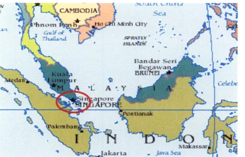
Singapore is an island nation in Southeast Asia, just South of Malaysia (Figure 2.1). CAMODIA

aquifers or

lakes and due to its small size, there is little space to store that water for use.

Malaysia to meet its water demand. The first treaty was signed in 1960 and expires in 2011,

-i , a ka r ta . a5e

Figure 2. 1: Map of Southeast Asia with Singapore Highlighted (My Travel Guide 2008)

Singapore was established as a British port in 1819 due to its location and function as a hub for trade with Iiated uand China. After World War whII, Britain felt that the country was too small to be a sovereign nation and instead granted it increasing liberties with time. Singapore joined the Federation of Malaya in 1963, but the union was short-lived due to internal conflicts. In contrast to the other federation members, Singapore's majority population was Chinese. This racial diversity spurred the call for a "Malaysian Malaysia," leading to several race riots in Singapore.

Singapore exited the federation and became an independent nation in 1965.

Singapore has 4.4 million people and a water demand of 1.36 billion liters per day (Madslien 2008). While Singapore receives a significant amount of rainfall-approximately 2400 millimeters per year (Tortajada 2006nds, it is considered water scarce. Singapore has no natural aquifers or lakes and due to its small size, there is little space to store that water for use.

Prior to becoming a sovereign nation, Singapore had negotiated treaties for water purchases from Malaysia to meet its water demand. The first treaty was signed in 1960 and expires in 2011, while a second treaty was signed in 1961 and expires in 2061. The two countries have already met to discuss the terms of new treaties that will take the place of these two once they have expired. However, Malaysia is demanding a price that is fifteen to twenty times higher than that negotiated under the previous contract, which was S$0.026 per ten cubic meters (Tortajada 2006).

(8)

self-sufficiency by 2061, such that when the treaties on water exchange with Malaysia expire, there will no longer be a need to import water. Recognizing that meeting the country's water needs can be viewed as a problem of insufficient supply or one of high demand, the Public Utilities Board (PUB) has taken actions to both increase Singapore's internal water supply and to reduce the national water demand through a strategy known as "Water for All: Conserve, Value and Enjoy." By taking this two-pronged approach, Singapore is well on its way to becoming self-reliant in terms of its water needs.

The campaign for increasing supply is referred to as "Water for All." Singapore meets its water needs through a 'Four Taps' Strategy, with the four sources being: water imported from Malaysia, rainwater from local catchments, reclaimed wastewater (called 'NEWater'), and desalinated seawater. As of May 2007, approximately 40% (Morris 2007) of Singapore's water supply was coming from Malaysia. By increasing the capacity of the other three taps, all of which come from within the country, Singapore can reduce the percentage that is coming from Malaysia and thereby reduce its international dependence for meeting its water needs.

Rainwater catchments are an important part of the water supply for Singapore. Stormwater is collected through a network of drains, canals, and river channels and directed towards one of the nation's fourteen reservoirs. These reservoirs currently collect water from about half of

Singapore's land surface. It is expected that additional catchments will be built by 2011 to bring the total catchment area from one half to approximately two thirds of the country's land surface. PUB has also taken measures to improve the quality of the water in the catchments through pollution controls such as public and private sewer maintenance, silt controls, regulation of industry, and gross pollutant traps. Each of these measures helps to improve water quality in the catchments by improving the quality of the water before it reaches the reservoir.

An important part of the "Conserve, Value and Enjoy" campaign is the ABC Waters Programme. PUB launched the ABC Waters Programme in an effort to achieve national waters that are active (open for different recreational activities such as boating or fishing), beautiful (aesthetically pleasing in a way that the nation's inhabitants can enjoy), and clean (of sufficient quality for domestic, industrial, and recreational uses). By improving the quality, aesthetics, and access to Singapore's waterways, PUB hopes to foster a greater sense of ownership and respect for water in Singaporean communities.

(9)

3 Site Description

Singapore is divided into three main catchment areas: the Western Catchment, the Central Catchment, and the Eastern Catchment. This study focuses on watershed management for the Kranji Reservoir and Kranji Catchment (Figure 3.1), which are located in the Western Catchment. The Kranji Catchment and Reservoir are in the northwestern corner of the island (1025'N, 1030_43'E).

Figure 3. 1: Map of Singapore with Kranji Reservoir Highlighted (GoogleMaps 2008)

The Western Catchment encompasses the western third of the country and is home to about one million people or 27% of Singapore's total population (PUB 2008b). The catchment remained largely undeveloped until after Singapore achieved independence (PUB 2008b) and is currently an approximately equal mix of urban development, industrial development, and natural environment (PUB 2008a). Residential areas are concentrated on the southern edge of the catchment (PUB 2008b).

The Kranji Reservoir was created in 1975 by the damming of an estuary from the Johor Strait that separates the Malaysian mainland from Singapore. The reservoir is approximately 647 hectares in area and the catchment has four tributaries, Kangkar River, Tengah River, Peng Siang River, and Pangsua River.

The Kranji Catchment is approximately 6076 hectares in area. It is mostly undeveloped with some rural and manufacturing industry (PUB 2008b). Most of the land around the reservoir is designated as open space under current zoning regulations, with the exception of some agricultural land use, a small golf course to the west, and some light industry to the east (PUB 2008b).

While the Kranji Reservoir is strong in many aspects (including beauty, ecological uniqueness, and open spaces), the Western Catchment Masterplan (PUB 2008b) states that the Kranji sub-catchment currently has low visiting rates because of a combination of factors. First, the site is

(10)

relatively isolated since most of the sub-catchment is undeveloped. Second, public transportation is limited. Third, there are only two entry points (one on either side of the dam) and poor connectivity within the site. Finally, public recreational activities are limited. Current recreational opportunities include cycling, park visits, and minor fishing areas.

A proposal for improvements to the Kranji Reservoir has been made under the "Western Catchment Masterplan" (PUB 2008b). The proposed changes would be primarily made to the existing entrances to boost low visiting rates while still preserving the rich natural resources. The addition of a Kranji Reservoir Visitor Centre west of the dam will provide educational information and experiences on the wetlands and the reservoir. Minor changes to vegetation at the intake will also prime the location for bird watching and a bird observation tower. Also, the introduction of an electric 'eco-cruise' boat will help increase connectivity within the site.

Water quality improvements (through wetland construction near the intake channel) will enable kayaking along the water side and better fishing, barbecue, and picnic facilities east of the dam. PUB would like to increase recreational activities on the Kranji Reservoir further, but more information is needed about bacteriological levels in the water before activities that involve higher degrees of contact with the water can be introduced.

(11)

4 Previous Study of Kranji Reservoir

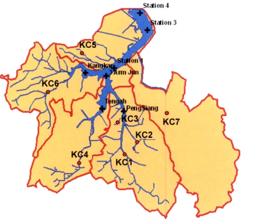
The Public Utilities Board (PUB) of Singapore would like citizens to be able to use Kranji Reservoir for a wider variety of recreational activities. The currently elevated bacterial loadings of the reservoir prohibit this type of use. Watershed protection efforts have already begun in many of the island nation's other catchments. Work investigating the Kranji Catchment by Nanyang Technological University (NTU 2008) in Singapore has focused on analysis of the water quality in the catchment. This analysis made use of seven sampling stations in the catchment and seven sampling stations within the reservoir, as seen in Figure 4.1. The study measured E. coli and Enterococci densities as the indicator bacteria for water quality. Table 4.1 presents the E. coli results from the NTU study. USEPA guideline concentrations for recreational waters can be expressed as a combination of single-sample maximum values and geometric means. Because Singapore's government does not have guidelines for E. coli levels, the NTU study used USEPA guidelines. The bold values in Table 4.1 indicate locations that exceed

USEPA values (USEPA 1986).

Table 4.1: Kranji Reservoir and Catchment E. coli Data (Sept. 2005 to Sept. 2007) (NTU 2008)

E. coli Density (MPN/100ml)

Geometric Standard

Location Minimum Maximum Mean Deviation Sample Size Reservoir Sampling Locations

Station 1 1 530 18 150 17 Station 3 1 130 3.4 34 17 Station 4 1 140 3.5 33 14 3 Arm Junction 1 1,800 20 480 17 Peng Siang 8 2,400 100 840 14 Tengah 2 200 17 70 16 Kangkar 1 700 14 170 10

Catchment Sampling Locations

KC1 110 24,000 2,300 5,700 17 KC2 1,300 >24,000 7,700 9,600 17 KC3 130 6,900 630 2,200 14 KC4 50 8,300 320 2,000 17 KC5 1,300 24,000 2,200 6,600 14 KC6 310 4,100 1,600 980 16 KC7 630 13,000 1,200 4,000 10

Note: Bold values exceed USEPA guidelines.

Table 4.1 shows that in the main body of the reservoir, the geometric means of the indicator bacteria fell below USEPA guidelines for every location. Stations 3 and 4, which are located at the north end of the reservoir, had the lowest geometric means. Even with acceptable geometric means, the reservoir water samples exceeded the single-sample maximum values for E. coli in four of the seven reservoir sampling locations. The single-sample maximum values were exceeded for both primary contact recreation and secondary contact recreation. The monitoring

(12)

stations located in the catchment had very high bacteria counts, exceeding USEPA guidelines for both geometric means and single-sample maximums at every location.

Figure 4.1: NTU Catchment and Reservoir Sampling Locations

The NTU study determined event mean concentrations (EMCs) for a variety of nutrients in seven sub-catchments, KC1 - KC7. (Please note that the naming convention for the sub-catchments in the NTU Study was CP. In our study, this has been replaced with KC (Kranji Catchment), as this is the most recent naming convention.) The NTU (2008) study collected samples that were analyzed for: ammonia (NH₃), nitrogen (N), nitrate (NO3), nitrite (NO2), total dissolved nitrogen

(TDN), total nitrogen (TN), chlorophyll-a (Chl-a), total suspended solids (TSS), phosphate (PO4), total dissolved phosphorous (TDP), total phosphorous (TP), TN/TP, silicon dioxide (SiO2), total organic carbon (TOC), dissolved organic carbon (DOC), total inorganic carbon

(TIC), and particulate organic carbon (POC). The contributors to the NTU study also mapped land use in each catchment, as seen in Figure 4.2. As seen in Table 4.1, the KC2 sub-catchment had the highest levels of E. coli. KC5, KC1, and KC7 had substantially higher levels of E. coli than the remaining three sub-catchments. The study found that high bacterial loadings, as demonstrated by high levels of indicator bacteria, were correlated to a high percentage of development in the sub-catchment, as seen in Table 4.2.

(13)

Table 4.2: Land Use of Five Sub-Catchments and Mean Bacterial Concentration (NTU 2008)

Station Location Mean E. coli Percentage Percentage (MPN/100 mL) Developed Impervious KC1 Bricklands 3,900 33 25 KC2 CCK AVE4 12,000 71 28 KC4 TG Airbase 1,200 1 0 KC6 AMK1 1,500 20 17 KC7 Sg Pangsua 3,500 40 23 * Sampling location

Residential land use

iGrass

land

Recreational land use Agrculture or

horticulture land use

Undeveloped

Figure 4.2: Land Use Map of the Kranji Catchment Exclusive of KC7 (NTU 2008) (KC7 is shown in Figure 4.1 and consists largely of residential land use.)

The study of the Kranji Catchment also indicated that storm events contributed more bacteria to the water passing each station than did dry weather. This is to be expected, as higher bacteria levels are strongly associated with the first flush phenomenon, during which a storm event washes accumulated bacteria on the surface into the drainage system immediately. These findings demonstrate the need to examine the residential contribution to bacterial loading in the catchment. The bacteriological contribution of the individual sewage treatment plants in the catchment, of which there are 47 (Figure 4.3), also needs to be examined. The NTU study indicated the need to sample wet-weather as well as dry-weather concentrations.

(14)

Figure 4.3: Kranji Catchment Sewage Treatment Plants (STPs) (Chua 2008)

The findings from the NTU (2008) study have contributed significantly to the knowledge of the catchment's characteristics and the bacterial loadings of the sub-catchments to Kranji Reservoir. Our study builds upon the findings of the NTU (2008) study by determining the bacterial contributions resulting from point and non-point sources in the sub-catchments and evaluating the fate and transport of the bacteria to Kranji Reservoir.

(15)

(16)

5 Scope of Study

This study sought to characterize the E. coli concentrations in the drainage system in the Kranji

Catchment and the attenuation experienced by the E. coli while traveling through the drainage

system and being held in Kranji Reservoir. To this end, we conducted field and laboratory work during January 5-23, 2009 to measure E. coli concentrations within the catchment and reservoir.

We analyzed the data using first-order decay modeling, ArcGIS's ArcMap (ESRI 2008), and USEPA's Water Quality Analysis Simulation Program (WASP) (Wool et al. undated). The first-order decay model incorporated decay due to settling, natural mortality, and photolysis, as applicable. We used ArcMap to calculate distances in the catchment, which we then used to compute attenuation. We employed WASP to simulate the fate and transport of E. coli within the reservoir.

The objective of our fieldwork was to determine probable sources of bacterial contamination to the reservoir and catchment by sampling different locations around the catchment to find the highest concentrations of bacteria. The objective of our attenuation modeling was to determine if the bacteria from the sources found in the fieldwork die off substantially before reaching the reservoir. Locating where the highest concentrations of E. coli exist and whether or not these

sources contribute high levels to the reservoir are important in determining appropriate measures to control the bacterial concentrations within the catchment. This also allows PUB to rank the importance of the sources that add bacteria to the reservoir.

The objective of our GIS analysis in sub-catchment KC2 was to determine future sites of additional study. We found possible areas of E. coli sources that can be sampled in future studies

to characterize more fully the sub-catchment's bacterial loading.

The objective of our WASP modeling was to create a representation of the reservoir and catchment system to determine how it generally behaves. This will allow PUB to determine which areas of the reservoir might experience higher E. coli concentrations depending on the

input of bacteria from the surrounding catchment and on the bacterial levels found in the reservoir upon sampling.

(17)

6 Fieldwork

6.1 Non-Point Source Sampling

Non-point sources of bacteria are characterized by the lack of specific origination points of the pollution. The NTU study indicated that residential runoff, a common non-point source, was a significant contributor of bacteria to the drainage system and, therefore, the reservoir (NTU 2008). We further explored these conclusions by collecting non-point source samples around the catchment in the drainage system.

6.1.1 Methods

Our team spent eleven days in January, 2009 taking 122 non-point source samples around the catchment, either via auto-samplers or grab-sampling. The auto-samplers were installed by NTU previously and collect samples from their locations by sucking water through a tube and depositing it in one of 22 bottles. The samplers also measure water level, rainfall, and stream velocity. They can be set to take samples at specific times or used to take a sample immediately. Grab sampling entails a team member collecting a sample in a Whirl-Pak bag by hand. To account for potential water quality changes due to diurnal variations in flow, we sampled sites at different times during the day and took a 22-hour round of hourly samples at KC2's auto-sampler, which is in a sub-catchment known to have high bacterial concentrations (see Figure 4.1 for location). For each sample, approximately 400-500 milliliters of surface water were collected in sterile plastic bags, chilled while being transported to the NTU laboratory, processed using membrane filtration and the Hach m-ColiBlue24® method within thirty hours, and incubated at 35 degrees Celsius for 23-25 hours. No appreciable precipitation occurred during the three weeks of fieldwork; therefore, no precipitation values were noted in the sampling.

We measured water temperatures at nine sampling locations within the catchment with a thermometer. We also measured flow at several sampling sites using a portable flow meter, but had reason to believe that the flow measurements were inaccurate and elected not to use them. We, instead, used flow and water-depth measurements from the auto-samplers' built-in flow meters, taking the average of January's data during the time we were conducting field work (January 7-22) as seen in Table 6.1. We expect these average values to be reasonably representative of flow during the entire period because of the lack of rainfall during our three weeks of field work. To illustrate this fact, we plotted the depths and velocities (in blue) with their averages (in orange) in Figure 6.1 and Figure 6.2, respectively. These graphs show that most of the data points lie near the averages. The outliers on January 14 are the result of a short rain event that is not representative of the three weeks, as seen in Figure 6.3. For our analysis in

Section 10 below, the averages are a suitable estimate for use in computation.

Table 6.1: Auto-Sampler Flow Measurements

Station Dates Average Velocity Average Depth Velocity Standard Deviation Depth Standard Deviation

(m/s) (m/s) (m) (m)

(18)

0.2 0.18 0.16 0.14 0.12 0.1 0.08 0.06 0.04 0.02 0 1/11 1/13 1/15 1/17 Average Depth 1/19 1/21 Date

Figure 6.1: Channel Depth at KC2's Auto-Sampler

Average Velocity

0

1/7 1/9 1/11 1/1

Figure 6.2: Velocity at KC2's Auto-Sampler

0.8

3 1/15 1/17 1/19 1/21

Date

Figure 6.3: Rainfall at KC2's Auto-Sampler 6.1.2 Sampling Locations

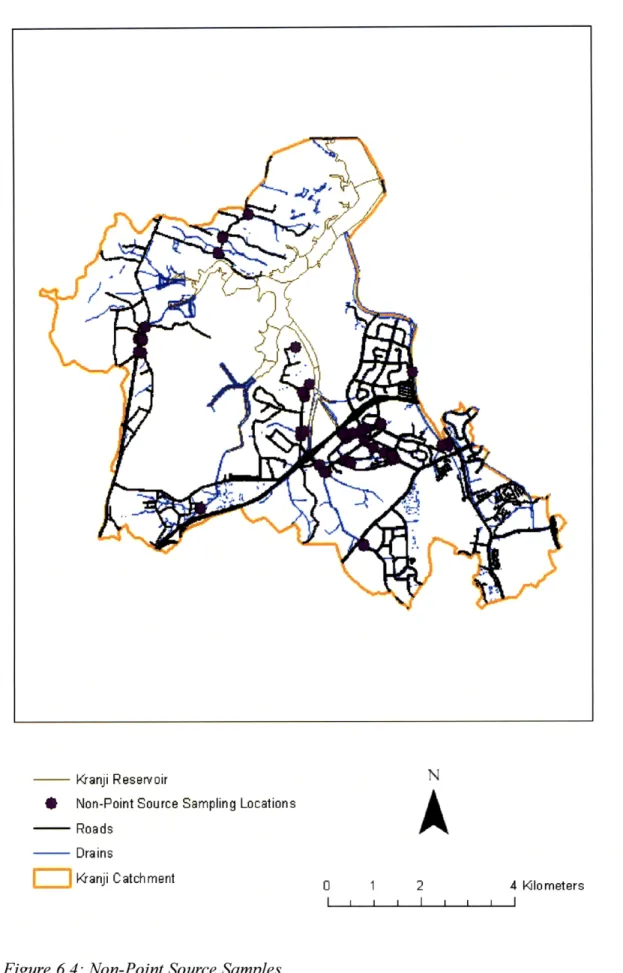
Our team took approximately 122 non-point source samples within the Kranji Catchment, at auto-samplers, within the drainage system, and from run-off at a fish farm and a chicken farm. Sampling locations are shown in Figure 6.4.

0.6 0.5 0.4 0.3 S0.2 > 1/7 1/9 1/11 1/13 1/15 1/17 1/19 1/21

(19)

Kranji Reservoir

* Non-Point Source Sampling Locations - Roads Drains SKranji Catchment

N

0 1 2 4 KIlometers I I I I l l I

(20)

6.1.3 Observations

In several of the sampling locations we made field observations, such as sheens on the water's surface or a sewage smell at the sampling site. These observations are included in the notes section in Appendix A. The sewage smell indicates that sanitary wastewater may be infiltrating the drains at these locations. This sewage smell may also be a product of people defecating in the drains. More study is needed to determine the exact causes of the sewage smell in these areas. The sheens may indicate small gasoline spills or road run-off getting in the drains. More study should be done to determine the sources of this potential contamination as well.

6.2 Point Source Sampling

Prior to our study, PUB suspected sewage treatment plant (STP) overflows to be the main source of bacterial pollution. Our team's point source sampling sought to determine the impact of a select few STPs within the catchment on the reservoir's and drainage system's bacterial loading. 6.2.1 Methods

We collected five point source samples from the effluent and influent of three STPs on January 20, accompanied by PUB officials. During sampling, approximately 400-500 milliliters of effluent from the septic or sedimentation tanks at these STPs were collected in sterile plastic bags, chilled until transported to the NTU laboratory, processed using membrane filtration and the Hach m-ColiBlue24® method within thirty hours, and then incubated at 35 degrees Celsius for 23-25 hours.

6.2.2 Sampling Locations

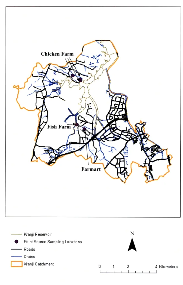
Our team sampled at selected STP effluent discharge points and one influent to an STP identified by PUB. We collected the five samples at three locations within the Kranji Catchment including a produce market/restaurant complex (Farmart), a very large chicken farm, and a fish farm. The

(21)

- Kranji Reservoir

* Point Source Sampling Locations --- Roads SDrains SIKranji Catchment

i

0 1 2 4 kilometers I I I I I I

(22)

6.3 Reservoir Sampling

This section was written as part of a collaborative effort with Cameron Dixon.

Reservoir sampling occurred over the week of January 19 through January 23. We conducted the sampling to determine bacteria levels in the reservoir itself.

6.3.1 Methods

Our team collected water samples from a boat provided by PUB, using either Whirl-Pak bags or clean, sterile 1-liter containers for sample collection. We first removed the cap or opened the bag, and then placed the mouth of the container approximately ten centimeters beneath the surface of the water until the container was nearly full. We then sealed the pre-labeled container and placed it on ice in a cooler in the boat. The samples were kept on ice until analysis in the laboratory. Fourteen samples taken on January 19 and 20 were tested for E. coli by membrane filtration. The high turbidity of the reservoir rendered the samples unable to be analyzed using membrane filtration. Because of this, we discontinued E. coli testing after the second day.

6.3.2 Sampling Locations

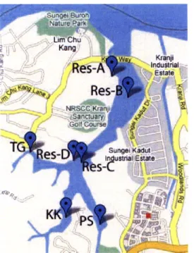
Our team took water samples from select locations distributed within the reservoir. Figure 6.6 shows the sampling locations in the reservoir. Res-A is where the proposed boat launch and visitor's center will be located. Res-B and Res-C are in the same places as Station 3 and Station 1 from the previous reservoir study by NTU (2008), as can be seen in Figure 4.1. Res-D is located next to the proposed pavilion and dock. We chose sampling locations TG, KK, and PS to allow us to characterize their respective inflow arms of the reservoir.

(23)

6.4 Domestic Wastewater Infiltration Testing

We conducted testing for inadvertent domestic wastewater hookups to drains using cotton pads to adsorb whiteners from detergent products carried in domestic wastewater. These whiteners fluoresce when held under a black light. We placed cotton pads in four drains in KC2 carrying reservoir-bound flow and left them for two days. We removed the pads and analyzed them for fluorescence under a black light. Any fluorescence would have likely been due to laundry detergents and, thus, would have indicated that human wastewater was contributing to the drain's flow. Due to the cotton pads also attracting a substantial amount of particulate matter, we could draw no conclusions from this test even after pulling them apart and rinsing them to try to remove some of the particulate buildup.

(24)

7 Laboratory Analysis

Our team completed three weeks of sampling, resulting in 148 samples, including seven blank samples. We used the Hach m-ColiBlue24® method to process the samples in order to delineate

E. coli concentrations. This is a membrane filtration test that allows enumeration of total

coliform and E. coli (fecal coliform) within 24 hours. After incubation, total coliform colonies appear red and E. coli appear blue and can be counted (Hach Company 1999).

We determined the reservoir E. coli levels using membrane filtration and the Hach m-ColiBlue24® method, but, because of the reservoir's high turbidity, E. coli levels at those sampling sites are uncertain. Because some dilutions of the samples showed no E. coli colonies, however, an upper limit can be determined for the E. coli concentration of those samples.

We used the resulting bacterial colony counts to find the waters' total coliform and E. coli concentrations, based on the dilution used in the analysis. We mapped all of the sampling locations using GIS.

7.1 Preliminary Results

Total coliform concentrations ranged from 1800 in a KC2 drain to 167 million in the run-off of a fish farm. E. coli concentrations ranged from 87 in a KC2 drain to 29 million at a location draining directly into the reservoir downstream from KCI's auto-sampler. A selection of the sampling results can be found in Table 7.1. The complete results including duplicates and blanks can be found in Appendix A. Maps of the results can be seen in Figure 7.1 (for non-point sampling results) and Figure 7.2 (for point source sampling results).

Table 7.]1: E. coli Concentrations at Selected Sampling Points

Sample Name Date Time E. coli Concentration Location (CFU/100 mL)

22.7-44.8-A 01/12/09 11:34 520,000 KC2 Drainage System 22.8-44.7 01/09/09 12:50 9,000 KC2 Drainage System 22.9-44.3-18 01/22/09 18:00 2,300 KC2 Drainage System 22.9-44..3-1 01/22/09 01:00 150,000 KC2 Drainage System

23.8-43.4-A 01/20/09 16:00 830,000 Chicken Farm Sedimentation Tank Entrance 23.8-43.4-B 01/20/09 16:05 <1201 Chicken Farm Sedimentation Tank Exit

23.0-43.6 01/20/09 17:55 >200,000,0002 Farmart Sedimentation Tank Exit 23.2-43.3 01/20/09 17:15 1,500 Fish Farm Sedimentation Tank Exit

25.0-43.1 01/20/09 15:15 3,700 Chicken Farm Sedimentation Tank Exit

This number is an estimate. The sample showed zero E. coli for a 1:100 dilution. Neither a 1:1 nor a 1:10 dilution was performed. The test performed is only valid for E. coli counts between 12 and 200.

2 This number is an estimate. The sample showed greater than 200 E. coli for a 1:1,000,000 dilution. No higher dilutions were analyzed. The test performed is only valid for E. coli counts between 12 and 200.

(25)

E. Coil (CFUI100 mL) * 0-200 * 200-2,000 0 2,000 - 20 D00 * 20,000 -200 D00 0 2000,000- 200,000,000 - anji Reservoir - Roads - Drains I Kranji Catchment N

A

0 1 2 4 Kilometers II I I I 1 I I

Figure 7.1: Non-Point Source Sampling Results

(26)

E. Coli (CFUII00 mL) I 0-200 * 200-1,500 0 1,500 - 4,000 * 4,000- 800,000 * 800,000 - 200,000,000 - Kranji Reservoir _N -- Roads SDrains

J

IKranji Catchment 0 1 2 4 Kilometers I I I I I I I

(27)

We also conducted a 22-hour round of sampling at auto-sampler KC2 to evaluate the variability of E. coli concentrations over time. This test showed that E. coli concentrations can vary substantially over time, as seen in Figure 7.3. This variability could also be a result of intrinsic variability in bacteria sampling.

160000 140000 120000 100000 80000 60000 40000 20000 0

I

I==m..

1 .

.

__

14:00 16:00 18:00 20:00 22:00 0:00 2:00 4:00 6:00 8:00 10:00 Time of Day Figure 7.3: 22-Hour Round of Sampling at KC2's Auto-Sampler

The reservoir E. coli readings are shown in Table 7.2. Due to high turbidity in the reservoir, we could not read the non-diluted samples. These E. coli concentrations are based on the fact that samples diluted one-to-ten showed no E. coli. These concentrations are estimates.

Table 7.2: Reservoir Sampling Data

Date 01/19/09 01/20/09

Sample Name E. coli Concentration (CFU/100 mL)

23.7-43.4 <10 <10 23.9-44.0 <10 <10 24.7-43.7 <10 <10 24.7-43.5 <10 <10 24.8-42.8 <10 <10 25.9-44.5 <10 <10 26.1-44.2 <10 <10

(28)

8 Field and Laboratory Quality Control and Quality Assurance

This section was written as part of a collaborative effort with Carolyn Hayek, Cameron Dixon, and Jean Pierre Nshimyimana.

Quality assurance (QA) is the standard program and policies adopted for field and laboratory operation that define the measures necessary to produce defensible data of known precision and accuracy. Quality control (QC) is the set of processes adopted to ensure the quality of analytical data produced (Eaton et al. 2005).

8.1 Initial Demonstration of Competency

Each member of our research team completed an initial demonstration of capability to conduct each test that was performed in this project (Eaton et al. 2005). We examined our field and laboratory notes to ensure that every member of our team used the same protocols and found no inconsistencies.

8.2 Collection and Preservation of Samples

The MIT research team collected samples that were small enough by volume to be transported to the lab easily but still large enough to be used in the analysis, ranging from 400 milliliters to one liter. We handled samples in a way that prevented deterioration, contamination, or any other result that would have compromised them before analysis, by collecting them in sterile Whirl-Pak bags or 1-liter bottles and transporting them in coolers with ice. We made certain of the cleanliness and quality of all sampling equipment and used only clean sample containers. Following the procedures of Eaton et al. (2005), all bottles being reused were either bleached and soaked in deionized water or baked at 450 degrees Celsius to ensure cleanliness.

Following procedures from Eaton et al. (2005), we filled sample containers without pre-rinsing with sample, leaving a space for aeration. To minimize the potential for biodegradation, samples were then chilled, but not frozen, in coolers until transported to the laboratory.

8.2.1 Proper Labeling

Our team made a record of every sample collected and identified each bottle/container with a unique sample number, team name, sample type (if DNA), date, hour, minute and exact location collected, which were written on the sample's label. Other data such as water temperature, weather conditions, water level, and stream flow were recorded in the field logs. We used GPS to determine sample locations.

8.2.2 Laboratory and Field Blanks

A blank is a water sample that has no initial concentration of bacteria. This blank is used to evaluate instrument performance and the accuracy of testing. We took blank samples with our sample batches on the third, fourth, fifth, sixth, and seventh days of sampling. On these days, we took approximately one blank sample for every eight field samples. All blanks contained zero E.

(29)

coli and zero total coliform, as can be seen in Table 8.1, demonstrating the lack of outside

contamination experienced by the samples in the study.

Table 8.1: Laboratory and Field Blanks

Sample Total Coliform Total E. coli Date Name Time (CFU/100 mL) (CFU/100 mL)

1/12/2009 Blank 12:55 0 0 1/12/2009 Blank 11:38 0 0 1/13/2009 Blank 14:30 0 0 1/14/2009 Blank 11:08 0 0 1/14/2009 Blank 12:30 0 0 1/15/2009 Blank 11:50 0 0 1/16/2009 Blank 12:43 0 0 8.2.3 Duplicate Sampling

At specific sampling sites, our team took two samples (a sample and a duplicate sample). Following the procedures of Eaton et al. (2005), the duplicate sample was taken in the field in the same way the original sample was taken. The duplicate was processed in the laboratory like the original sample was processed. We took duplicate field samples with our sample batches on the second, third, fourth, fifth, sixth, seventh, and tenth days of sampling. On these days, we took approximately one duplicate sample for every nine field samples, resulting in ten duplicate samples.

We evaluated our duplicate samples based on quality assurance goals published by Oregon's Department of Environmental Quality (2001). To achieve these goals, the relative percent difference between the original sample and the duplicate sample should be less than 25 for samples with values greater than five times the detection limit, or sixty Colony Forming Units per one hundred milliliters. For samples with values less than or equal to sixty Colony Forming Units per one hundred milliliters, the absolute difference between the same dilution of the two samples should be less than two times the detection level, or 24 Colony Forming Units per one hundred milliliters. If our samples do not achieve these goals, we have qualified them with a J, indicating they are an estimate.

To analyze the accuracy of our duplicate sampling, we used Equation 8.1 (Eaton et al. 2005) to calculate the relative percent difference of the two samples with the same dilution, as seen in Table 8.2. We also calculated the absolute difference of the two samples with the same dilution, as applicable, as seen in Table 8.2.

[original]- [duplicate] x100 (8.1)

(30)

Table 8.2: Duplicate Samples

Date Sample Time E. coli Dilutions Total E. coli Relative Absolute Qualifier

Name 102 103 104 106 (CFU/100 Percent Difference

mL) Difference (CFU/100 mL) 1/9/2009 22.9-44.3-D 10:30 34 21 1 12,200 NA3 13 1/9/2009 22.9-44.3-D 10:30 47 0 1 4,700 1/12/2009 22.7-44.9-B 11:50 TNTC TNTC 158 1,580,000 NA 155 J4 1/12/2009 22.7-44.9-B 11:50 TNTC 17 3 17,000 1/13/2009 22.6-44.4-A 14:25 18 5 0 1,800 NA 75 1/13/2009 22.6-44.4-A 14:25 11 2 2 uncertain 1/14/2009 22.7-44.9-B 10:35 10 1 0 uncertain NA 35 1/14/2009 22.7-44.9-B 10:35 7 0 0 uncertain 1/14/2009 23.0-43.8-B 12:27 TNTC TNTC TNTC TNTC 06 NA7 1/14/2009 23.0-43.8-B 12:27 TNTC TNTC TNTC TNTC 1/15/2009 24.0-42.0-D 14:55 6 4 0 uncertain NA 65 1/15/2009 24.0-42.0-D 14:55 0 0 0 uncertain 1/15/2009 21.7-44.5 11:50 37 4 0 3700 NA 7 1/15/2009 21.7-44.5 11:50 30 8 0 3000 1/16/2009 23.0-43.8-B 11:15 TNTC TNTC 29 29000000 NA 25 J4 1/16/2009 23.0-43.8-B 11:15 TNTC TNTC 4 uncertain 1/16/2009 22.6-44.4-A 12:45 21 0 0 2100 NA 115 1/16/2009 22.6-44.4-A 12:45 10 1 0 uncertain 1/21/2009 22.8-45.5-A 16:30 70 21 5 108500 NA 49 J 1/21/2009 22.8-45.5-A 16:30 21 7 4 2100

TNTC: Too Numerous To Count NA: Not Applicable

J: Estimated Value

3 The relative percent difference analysis is not applicable to values less than sixty Colony Forming Units per one

hundred milliliters.

4 One of the values is not in the valid range of twelve to two hundred; therefore, this absolute difference is only an estimate.

5 One or both of the values is not in the valid range of twelve to two hundred; therefore, the absolute difference is only an estimate.

6 The values are not in the valid range of twelve to two hundred; therefore, the relative percent difference is only an estimate.

7 The absolute difference analysis is not applicable to values greater than sixty Colony Forming Units per one hundred milliliters.

(31)

As the table demonstrates, only a single sample with E. coli values between twelve and two hundred (Sample 22.8-45.5-A) did not meet our quality assurance goals. This indicates the relative accuracy of our testing procedures. The discrepancies exhibited by sample 22.8-45.5-A and its duplicate can be attributed to errors in our sampling or analysis methods. They could also be the result of problems with our analysis media. Hach has discontinued sale of their m-ColiBlue24® broth due to lack of sensitivity in random testing of the product. Communication with Hach revealed that the discontinued m-ColiBlue24® gave lower than expected concentrations of E. coli (Hach Customer Service 2009); therefore, we have assumed that even if this is a problem in our study, our values are still valid, but may be taken as conservatively low. Another possible source of the discrepancies is the natural variation in bacteria concentrations in a water body. Fluctuations in concentration are more common in flowing water (e.g. streams and drains) which is where many of our samples were taken. Also, because duplicate sampling consists of taking two separate samples of the water, the second sample could have more sediment due to stirring of the water body while taking the first sample (Thompson 2009). These effects would contribute additional E. coli to a sample.

8.2.4 Split Sampling

Split sampling entails analyzing the same sample more than once. We did not conduct any split sampling in our analysis.

(32)

(33)

9 Theoretical Modeling of Bacterial Attenuation

9.1 Bacterial Attenuation through the Drainage System

The fate of bacteria in the environment has been studied extensively. Because E. coli is less sensitive to environmental stresses than other pathogens, it has been used in many of these studies as a conservative indicator of bacterial levels in recreational waters (Bowie et al. 1985). To find the expected attenuation as bacteria travel through the drainage system of Kranji Catchment, factors that influence bacterial die-off must be determined and modeled. These factors can be categorized as physical, physiochemical, or biochemical-biological (Bowie et al. 1985).

The physical factors that affect bacterial decay include photo-oxidation, adsorption, flocculation, coagulation, sedimentation, and temperature. Only photo-oxidation, or photolysis, temperature, and adsorption onto particles and sedimentation of those particles have been quantitatively shown to correlate to bacterial die-off. It has been postulated that ultraviolet light damages cell DNA, and, as such, sunlight kills off bacteria as effluent travels from the source (Bowie et al.

1985). Because much of the drainage system in Singapore is exposed to light, photolysis die-off

will have a significant effect on the attenuation of bacteria from their sources to Kranji Reservoir. Temperature is also an important contributor to die-off rates of bacteria as quantified by Mancini (1978). Sedimentation will also have a significant effect on the die-off of bacteria in the drainage system, and needs to be incorporated into a model of bacterial disappearance in Kranji Catchment and Reservoir.

The physiochemical factors that influence bacterial decay include osmotic potential, pH, chemical toxicity, and redox potential. Increased salinity enhances the ability of solar radiation to increase the decay rate of bacteria. While heavy metal content and pH appear to affect disappearance rates, the exact manner in which these mechanisms contribute to the overall decay rates of bacteria is difficult to quantify and not fully understood in some cases (Bowie et al. 1985). Because of this and the fact that Kranji Reservoir is a freshwater body, these physiochemical factors will not be considered when modeling bacterial die-off in the drainage system.

The biochemical-biological factors that affect the decay rate of bacteria include nutrient levels, presence of organic substances, predators, bacteriophages, algae, and presence of fecal matter (Bowie et al. 1985). While nutrient levels, predation, and algae appear to affect disappearance rates for bacteria, the synergies and mechanisms for these effects are not fully quantifiable. Except for the natural mortality effects on bacteria disappearance, these biological factors will not be incorporated into the attenuation model for Kranji Reservoir.

Traditionally bacterial die-off has been modeled using a simple first-order decay equation, as seen in Equation 9.1.

C, = Coe - k_i

(9.1)

In Equation 9.1, Ct is the concentration of bacteria at time, t. Co is the initial concentration of bacteria. The variable t is the time, and k is the decay constant.

(34)

The decay constant is typically determined experimentally using sample concentrations. The decay constant can also be found empirically, taking into account natural die-off, sedimentation, and photolysis, as discussed in Thomann and Mueller (1987). The total loss rate, k, is found by combining the loss rates for natural mortality, kl, photolysis, kp, and sedimentation, ks, as Equation 9.2 shows (Mills et al. 1985).

k = k + kP + ks _(9.2)

Bacteria naturally die just as any other living organism. This natural die-off needs to be incorporated into any rate constant for bacterial disappearance. Bacterial survival is heavily dependent on temperature, salinity, and solar radiation. Mancini (1978) developed a model to incorporate these factors empirically. Mancini used published mortality rates of bacteria and plotted decay rates versus temperatures to find a model that describes bacterial die-off in both seawater and freshwater. The rate constant for natural mortality of bacteria can be modeled with Equation 9.3, where T [degrees Celsius] is the water temperature (Mancini 1978).

k, = (0.8 + 0.006(%seawater))1.07(T-20)

(9.3)

Because Kranji is a freshwater reservoir and the drainage system of Kranji Catchment is presumed to have low salinity, the equation for natural mortality can be rewritten to exclude salinity, and the loss rate due to natural mortality, k, [per day], can be written as Equation 9.4.

k, = (0.8)1.07(T-2₀₎

(9.4)

As discussed above, ultraviolet light increases disappearance rates of bacteria. Thomann and Mueller (1987) developed an equation to describe die-off from photolysis using the findings of a study of the effect of sunlight on die-off rates of bacteria by Gameson and Gould (1974) and the fact that solar radiation is attenuated by water and, therefore, decreases with depth below the water surface. Light decay can be modeled with Equation 9.5, where a is a proportionality constant that has been determined by Thomann and Mueller (1987) from Gameson and Gould's data (1974) to be approximately unity. Iave [kilocalories per centimeter squared] is the average light energy experienced by the bacteria.

k = ave _(9.5)

Light energy, I, can be modeled with respect to the depth of water according to the Beer-Lambert Law, Equation 9.6, where Io [kilocalories per square centimeter] is the average daily amount of incoming light energy at the surface of the water. The variable ke [per meter] is an extinction coefficient dependent on turbidity (amount of particulate matter in the water) and color. The value of ke can be approximated as 0.55 times the concentration [milligrams per liter] of total suspended solids (TSS) in the water. The variable z [meters] is the depth below the water surface (Chapra 1997).

I(z)= Ioe-kez

(35)

For an open channel of depth H [meters], Iave can be found by integrating Equation 9.6 over the depth of the channel, as seen in Equation 9.7 (Chapra 1997).

1-e-k H

Ive = ave

1I

(9.7)

0kH

By incorporating these equations, a die-off constant due to photolysis, kp [per day], can be created. Thomann and Mueller (1987) did this as can be seen in Equation 9.8.

-ekeH

kP = a keH (9.8)

In addition to natural die-off and die-off due to photolysis, sedimentation of bacteria adsorbed to particles has an effect on the fate and transport of bacteria in a system. Bacteria can adsorb onto particles of sediment, which allows the bacteria to settle out of water as the particles settle. This settling loss rate is dependent on the fraction of bacteria that attaches to particles in the water, the settling velocity of these particles, and the depth of the channel. The loss rate due to sedimentation, ks [per day], can be modeled using Equation 9.9, where H is the channel depth. Fp is the fraction of bacteria that are attached to particles as modeled by Equation 9.10, and v, [meters per day] is the settling velocity of the particles (Chapra 1997).

V

k, = F, -- _(9.9)

The fraction of bacteria that adsorb to particles is dependent on the amount of particles in a water body, or the total suspended solids (TSS), and the partition coefficient associated with the bacteria and the particles involved. Equation 9.10 models the fraction of bacteria attached to particles. Kd [liters per milligram] is a partition coefficient and [TSS] [milligrams per liter] is the suspended solids concentration (Chapra 1997).

[TSS]Kd

= [TSS]Kd (9.10)

1+[TSS]Kd

Using the studies of Mancini (1978) and Thomann and Mueller (1987), die-off modeling can be done empirically for natural mortality, photolysis, and sedimentation. The drainage system in Kranji Catchment's KC2 sub-catchment was one-dimensionally modeled using the first-order decay equation (Equation 9.1), with the loss rate, k, incorporating natural mortality and sedimentation. This gives the attenuation from each sampling point to Kranji Reservoir via the drainage system.

9.2 Travel Time and Flow Data

(36)

(Equation 9.11).

R2/3S1/2

= h (9.11)

n

Rh [meters] is the hydraulic radius of the water in the channel and v [meters per second] is the

velocity of the flow in the channel. The variable, n, is the roughness coefficient that describes the roughness of the surface of the channel sides and bottom. So is the slope of the channel (Thomann and Mueller 1987).

Travel time for a parcel of water can be determined using Equation 9.12.

Sd

t v (9.12)

The variable d [meters] is the distance traveled and t [seconds] is the time taken to travel that distance. By measuring distances between sampling points and the reservoir in ArcMap, determining velocity through the system, and using Equation 9.12, we can determine travel time from the source to the reservoir.

(37)

10 Model Development

10.1 Assumptions

For our model development, we focused on sub-catchment KC2. We chose this one because we were able to take many more samples in KC2 than in any other catchment. Because this sub-catchment is mostly residential, there was easy access to many of the drains. This sub-sub-catchment was also highlighted in the NTU study (2008) as a suspected heavy contributor to the bacterial loading of the reservoir, since high concentrations of bacteria were found at its auto-sampler. Because KC2 is a newer residential area, the drain size and shape were relatively uniform throughout the drainage system.

For sub-catchment KC2, we made several assumptions regarding flow through the drainage system and the decay constant. Because the channels throughout the drainage system are relatively similar in cross-sectional area and depth, we assumed that the velocity of the water was constant in all parts of the drainage system. Because no substantial rain events occurred during the month and the standard deviation in the measured velocities was only 0.043 meters per second, we assumed the velocity of the channel was constant over time for our eleven days of fieldwork (January 7-22, 2009). We determined this velocity was approximately 0.2 meters per second, as seen in Table 6.1: Auto-Sampler Flow Measurements.

Because a very high percentage of KC2's drainage system is underground, the decay constant for KC2 did not include die-off due to sunlight, but only decay due to natural die-off and settling. Decay due to natural die-off (Equation 9.4) is dependent on water temperature. Because Singapore experiences relatively constant mean monthly temperatures, ranging from 26 degrees Celsius to 28 degrees Celsius throughout the year (The Weather Channel 2008), the water temperature in the drainage system can be assumed to be relatively constant. Based on observations and two temperature measurements in the covered drains, we assumed the water temperature to be constant at 26 degrees Celsius. Using this temperature, we computed the decay due to natural die-off as 1.2 per day.

To determine the decay due to settling (Equation 9.9), we estimated the average depth of water in the drainage system to be the average depth of water at KC2's auto-sampler, 0.06 meters, as seen in Table 6.1: Auto-Sampler Flow Measurements. Because there were no significant rain events during our field work, the standard deviation in the depth of the water in the channel was only 0.014 meters. Based on observations and depth measurements, we estimated that the depth of the water in the channels is relatively uniform throughout the drainage system. The particle settling velocity is 0.00002 meters per second, or about 2 meters per day, as approximated from a study by Jamieson (2005). The partition fraction was taken to be 0.44. This is the fraction of bacteria found to adsorb to 45-75 micron particles in Jamieson's study. Using this settling velocity, depth, and partition coefficient, we computed the decay due to settling in KC2 as approximately 10 per day, which dominates the decay constant.

10.2 Attenuation Model

The percentage of living bacteria as a function of time can be characterized by Equation 9.1. To describe the attenuation of the bacteria in KC2's drainage system, we combined the two

(38)

decay constants above. We computed the decay through the drainage system as 10 per day. The bacterial attenuation through the drainage system can be modeled with Equation 10.1. Distance,

d [meter], must be multiplied by the decay constant (approximately 10 per day) and divided by

the velocity (approximately 0.2 meters per second), which gives the coefficient of 0.0008 [per meter] in Equation 10.1.

C -0o.ooo0008d

1-- 1-e

Co (10.1)

This equation can be used to determine how much bacteria should be lost as bacteria travel through the drainage system of sub-catchment KC2. This can be used to predict bacteria levels within the system if all bacteria originate from a single source. This can, therefore, be used to

identify locations of potential bacterial sources. Locations that exhibit significantly higher bacteria levels than predicted by the model will indicate an area containing an additional bacterial source.

10.3 Model Verification

Lee Li Jun and Por Yu Ling, undergraduate students at Nanyang Technological University, conducted a test on March 25, 2008 to verify and calibrate our theoretical model. They collected two samples near KC2's auto-sampler. The locations of these points are shown in Figure 10.1. The results of this sampling can be seen in Table 10.1.

Figure 10.1: KC2 Sampling Points for Model Calibration (GoogleMaps 2009) Table 10.1: Model Calibration Sampling Results

Sampling Points E. coli Concentration Velocity (CFU/100 mL) (m/s)

Upstream Point 350,000 0.23

Downstream Point 190,000 0.23

The distance between these two points is approximately 150 meters. Using the velocity measured by the auto-sampler at 15:15 on March 25, 2009, 0.23 meters per second, we computed the travel time between the upstream point and the downstream point as approximately 11 minutes. Using

(39)

this travel time in Equation 9.1), we computed the bacterial decay constant, k, as approximately 81 per day to produce the die-off observed in the field. This is substantially more attenuation than our model predicts. Because this length of drain is exposed to sunlight, an additional 0.2 per day of decay (from Equation 9.8) would need to be added to our theoretical decay, however this is insufficient to explain the observed discrepancy between field observations and the attenuation rate computed in section 9. The additional attenuation observed in the field could be due to inaccuracies in the parameters, an incomplete theoretical model, or equation or sampling inconsistencies.

Because this test was conducted only once, we will use the theoretical decay constant of 10 per day in this study. This will give a conservatively low estimate of attenuation until further study can be done to fully calibrate the attenuation model of KC2's drainage system.