Damping identification and quantification: experimental evidences and first numerical results

HAL Id: hal-01633809

https://hal.archives-ouvertes.fr/hal-01633809

HAL is a multi-disciplinary open access archive for the deposit and dissemination of sci-entific research documents, whether they are pub-lished or not. The documents may come from teaching and research institutions in France or abroad, or from public or private research centers.

L’archive ouverte pluridisciplinaire HAL, est destinée au dépôt et à la diffusion de documents scientifiques de niveau recherche, publiés ou non, émanant des établissements d’enseignement et de recherche français ou étrangers, des laboratoires publics ou privés.

Thomas Heitz, Benjamin Richard, Cedric Giry, Frédéric Ragueneau, Alain Le

Maoult

To cite this version:

Thomas Heitz, Benjamin Richard, Cedric Giry, Frédéric Ragueneau, Alain Le Maoult. Damping identification and quantification: experimental evidences and first numerical results. 16th World Conference on Earthquake Engineering, Jan 2017, Santiago, Chile. �hal-01633809�

Registration Code: S-Y1463058271

DAMPING IDENTIFICATION AND QUANTIFICATION: EXPERIMENTAL

EVIDENCES AND FIRST NUMERICAL RESULTS

T. Heitz(1)_{, B. Richard}(2)_{, C. Giry}(3)_{, F. Ragueneau}(4)_{, A. Le Maoult}(5)

(1) _{Ph.D student, LMT-Cachan, ENS Cachan, CNRS, Université Paris Saclay, 61, avenue du Président Wilson, 94235 Cachan, France,} heitz@lmt.ens-cachan.fr

(2) _{Dr. Ing., CEA, DEN, DANS, DM2S, SEMT, Laboratoire d’Études de Mécanique Sismique. F-91191 Gif-sur-Yvette, France,} benjamin.richard@cea.fr

(3) _{Associate Professor, LMT-Cachan, ENS Cachan, CNRS, Université Paris Saclay, 61, avenue du Président Wilson, 94235 Cachan, France,} giry@lmt.ens-cachan.fr

(4) _{Full Professor, LMT-Cachan, ENS Cachan, CNRS, Université Paris Saclay, 61, avenue du Président Wilson, 94235 Cachan, France,} ragueneau@lmt.ens-cachan.fr

(5) _{Ing., CEA, DEN, DANS, DM2S, SEMT, Laboratoire d’Études de Mécanique Sismique. F-91191 Gif-sur-Yvette, France,} alain.lemaoult@cea.fr

Abstract

The way of quantifying energy dissipations in reinforced concrete (RC) structures during seismic events is still a complex issue to solve out. However, the designer would rather use simplified modelling for both the geometrical representation of the structure and its mechanical behaviour. To this end, the Rayleigh-type viscous damping based models are commonly used even if several studies have emphasized the inherent issues of this approach. Alternative solutions exist, but the target values of the damping themselves are still questionable since the dynamic properties of the structure evolve throughout the nonlinear time history analysis. To bring answers to the aforementioned issues, a set of experiments including seismic tests on RC beams is carried out by means of the TAMARIS experimental facility operated by the French Alternative Energies and Atomic Energy Commission (CEA). The results will be used to propose a new damping modelling strategy able to reproduce damping evolution throughout time history analysis while avoiding the use of complex constitutive laws. In this paper, the lacks of Rayleigh damping models are briefly reminded and a review of the advantages and disadvantages of various damping measurement experimental procedures is made. Then, the IDEFIX experimental campaign (not executed yet) is presented in contrast with the aforementioned review. Eventually, numerically simulated results of the tests are exposed and discussed. Preliminary numerical results in connection with the proposed damping modelling strategy will be shown and compared with the ones coming from existing approaches in order to demonstrate not only its relevance but also its efficiency.

Keywords: damping; RC structures; model identification; experimental campaign, Cast3M.

1. Introduction

Even though constitutive laws are now able to provide realistic and accurate results in the nonlinear domain behaviour of RC structure, the computational cost is a strong counterpart that designers and engineers are not always prone to pay for. For this reason, Rayleigh-based damping models as the classical one given in equation ( 1 ) are convenient and popular in the earthquake engineering community since it allows a fuzzy description of the dissipation sources occurring in the structure during the degradation process through a viscous force field.

𝑪 = 𝛼𝑴 + 𝛽𝑲 _{( 1 )}

Yet, even combined with refined inelastic analysis, the Rayleigh damping leads to unsatisfactory results from the physical point of view, as studied in [1]. Indeed, the resulting damping is overestimated when the initial stiffness matrix K0 is used in equation ( 1 ) throughout the time-history analysis for a damaged structure since the tangent stiffness decreased after cracking occurred. Moreover, the mass-proportional term does not have any physical meaning. Finally, the control of the damping level can be ensured on only two distinct frequencies.

It has also been shown that, under certain conditions, these drawbacks have a limited influence on the simulated structure response because according to [2] a linear viscous damping coefficient c1 model is able to represent with an acceptable accuracy the dissipations of a more general nonlinear viscous damping force Fd:

𝐹𝑑= ±𝑐𝑛 (

𝑑𝑥 𝑑𝑡)

𝑛

( 2 ) Furthermore, this assertion stays reliable to a certain extent, whether viscous [3] or non-viscous phenomena [4] are involved.

For these reasons and excepted the issues inherent to the Rayleigh damping model expressed earlier, the viscous damping models are still of interest, but two questions remain opened: “What damping ratio should be set for each eigenmode defining a given structure?” and “How should these damping ratio evolve throughout the inelastic time history analysis?” Several experimental campaigns have been carried out over the past decades in order to bring some answers to these questions. Different types of specimens have been tested: beams, columns, shear walls, joints and even large-scale structures. Besides this, four types of loadings have mainly been used:

1. quasi-static cyclic tests,

2. experimental modal analysis at different damage states, 3. free vibrations tests,

4. dynamic excitations studies.

An example of the first type of test is given in [5], the objective was to measure the energy dissipation during one cycle. By means of an energy equivalence principle developed in [6], an “equivalent viscous damping” could be estimated. In other words, the choice was made to describe the hysteretic dissipations occurring during a quasi-static test by a viscous force field (i.e. proportional to the velocity field). This lack of physics was counterbalanced by introducing a damage level dependence within the framework of a one-degree-freedom (DOF) state model. Another problem related to the quasi-static tests as they are performed traditionally is that it does not activate the inertial contributions or the dependence of damping on the frequency.

The second aforementioned strategy is more acceptable since the dissipations are assessed through a dynamic excitation (such as hammer shock tests or low-intensity white noise signals) that does not significantly, or not at all, modify the dynamic properties of the structure. This method is also able to provide information on the damage level as well as a rather accurate location of the defects, as shown in [7] or [8]. However, some phenomena are not activated at low levels: crack lips friction, debonding at the steel/concrete interface or crack propagation for example.

The third one is both dynamic and high level (decreasing from the prescribed displacement to the equilibrium state). Depending on the initial prescribed displacement field, which is directly related to a damage state of the structure, different phenomena may appear as in [9] or [10]. This test can provide relevant information related to the damping capacity of a damaged structure. However, some difficulties still arise. Several frequencies can be excited during the test, leading to a major difficulty in the data post-treatment. Especially, this is often the case when vibration modes are close to each other (mode coupling). Furthermore, the study of damping for higher frequencies is generally more and more difficult as a complex mode shape has to be imposed initially to the structure.

Finally, the fourth type of experiment (i.e. the ones including a dynamic loading) brings some answers to the aforementioned issues at the price of a more time consuming post-processing step. On one hand, in situ measurements are intrinsically the most representative of a real structure behaviour, but information about the boundary conditions and the structure’s environment are difficult to apprehend [11]. On the other hand, laboratory shaking tables provide an efficient way to reproduce seismic signals while having a rather good knowledge of the boundary conditions in comparison to in situ measurements. Limitations appear with the size of the structure to

characterize. Reduced-scale structures are often used [12] and discussions about the influence of the representative volume element of RC on the behaviour of the structure in such experiments are still in progress.

The difficulty to reproduce the damping occurring in RC structures during seismic events has been emphasized. An ideal test would involve a dynamic excitation with a wide frequency range and different accelerations levels. However, each test type previously described enabled a better understanding of some aspects of damping phenomena. Nowadays, the issue is more to analyse and quantify the interactions of the different parameters identified as being preponderant.

To tackle these challenges, an experimental campaign has been set up on RC beams by means of the AZALEE shaking table, as part of the TAMARIS experimental facility operated by the French Alternative Energies and Atomic Energy Commission (CEA). By using a shaking table and a RC beam element, the experiments take benefits from a dynamic excitation and allow overcoming the issue related to the scale effects. The experimental campaign will be first presented. Then, the main numerical results coming from finite elements simulations performed for the preparation of the experimental campaign are exposed and discussed. Eventually, preliminary numerical results of a new damping modelling strategy are shown and compared with the ones coming from existing approaches in order to show the relevance and efficiency of the proposed approach.

2. Experimental campaign: IDEFIX

This section describes the experimental campaign set up in this work. Two main objectives are aimed by this experimental campaign:

 to provide an identification method fulfilling the prescriptions of the last section with experimental data;

 to propose a new numerical description of damping, taking into account the structural state and the history of the specimen.

The tests are performed on a 6 x 6 m2 _{shaking table able to reproduce seismic signals up to 1.5 g, in a wide} frequency range, depending on the mass of the experimental setup. The table is controlled on 6 degrees of freedom (3 rotations, 3 translations). Characteristics of this experimental device are available in [13].

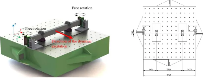
Fig. 1 – General view of the experimental setup and key dimensions in millimetres

To better understand and visualize the items described in the following subsections, a general view of the final experimental setup is presented in Fig. 1. A beam is mounted on AZALEE shaking table thanks to the elastic supports at its edges and the two additional masses over air cushions systems [14]. Please note that the input signals

act in the horizontal transverse direction of the beam (x-direction), meaning it is excited in its weakest flexural axis.

2.2 Samples

The name of this experimental campaign, IDEFIX, is a French acronym for “Identification of damping/dissipation in RC structural elements”. For the sake of simplicity and representativeness, the choice of RC beams has been made. Indeed, beams are probably the most usual structural components in civil engineering and the local stress states inside such components are well controlled. Numerous numerical beam models have been developed and offer accurate dynamic responses for reasonable computational time.

Keeping in mind one limitation observed in the tests performed by [5] (i.e. quasi-static tests), at least two eigenmodes of the beam should be considered in order to study mode interactions and the frequency dependence of the damping ratio. As mentioned in paragraph 2.1, shaking tables allow reproducing seismic signal in a relatively wide frequency band, depending on the boarded mass. In order to ensure a robust online control of the shaking table during the dynamic tests, the choice to keep the two first eigenfrequencies bellow 30 Hz has been made. This choice leads to a strong design criterion. In addition, a highly damaged state of the beam should be reached in order to quantify the influence of damage on the damping properties.

The final design of IDEFIX beams is given in Fig. 2 and the different cross-sections are described and pictured in Table 1. The 6 metres length of the beam corresponds to the width of the shaking table: the beam is the longest possible in order to decrease the second mode frequency (the effective span between supports is 5.90 m). For the same reason, additional masses of 360 kg each are mounted on the two first quarter-span from each end of the beam (see Fig. 1). The variants were defined to ensure the interface surface on one hand, and reinforcement ratios, on the other hand, are close to each other for two different pairs of cross-sections (10HA12 with 8HA16 and 8HA16 with 4HA20). The acronym “HA” means the presence of ribs on the reinforcement bars. On the contrary, “R” indicates the use of round and smooth steel bars. This last variant has been chosen to ensure the influence of ribs can be roughly estimated by comparison with the 10HA12 specimens. Two different types of concrete have been considered: C25/30 and C45/55 types (defined in Eurocode 2 part 3.1). Finally, the different types of specimens are reviewed in Table 2.

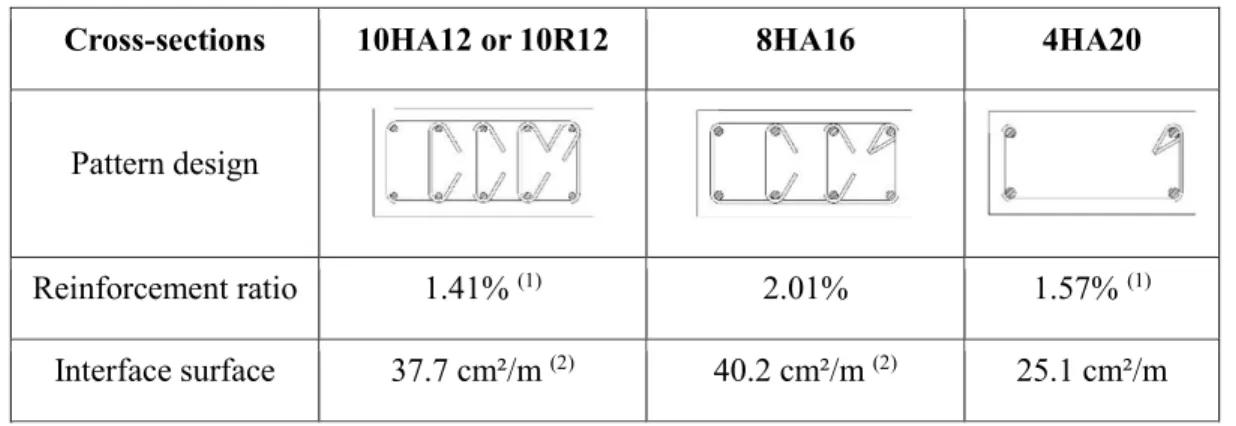
Table 1 – Cross section variants of the IDEFIX beam

Cross-sections 10HA12 or 10R12 8HA16 4HA20

Pattern design

Reinforcement ratio 1.41% (1) _{2.01% 1.57%} (1)

Interface surface 37.7 cm²/m (2) _{40.2 cm²/m} (2) _{25.1 cm²/m}

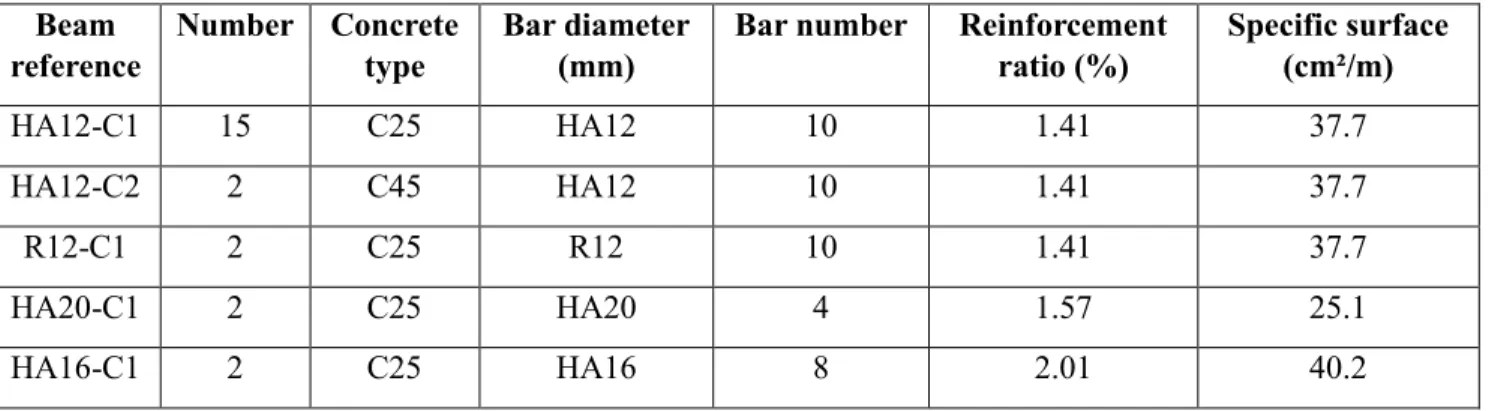
Fig. 2 – Dimensions of the IDEFIX beam – dimensions in centimetres Table 2 – Review of manufactured specimens.

Beam reference Number Concrete type Bar diameter (mm)

Bar number Reinforcement ratio (%) Specific surface (cm²/m) HA12-C1 15 C25 HA12 10 1.41 37.7 HA12-C2 2 C45 HA12 10 1.41 37.7 R12-C1 2 C25 R12 10 1.41 37.7 HA20-C1 2 C25 HA20 4 1.57 25.1 HA16-C1 2 C25 HA16 8 2.01 40.2 2.3 Experimental setup

The setup has been defined to ensure the beams are simply supported in the horizontal plane. The IDEFIX beams are excited along their weakest flexural axis. An original design has been chosen for the boundary conditions:

 blade-shaped supports meant to deform themselves elastically in order to allow the rotation at the beam extremities thus avoiding dissipations and noise during the measures,

 two air-cushion systems to bear the beam weight and to reduce drastically the friction between the beam and the shaking table’s upper plate. Those cushions work like hovercrafts and should not be confused with traditional air-cushions which are not meant to move globally.

2.4 Loading

2.4.1 Quasi-static loading

Series of quasi-static tests stand as references for the following dynamic tests similarly to the push-over method. Two procedures are considered: a classical four points bending tests (4PBT) operated by two actuators and a so called “S” bending test using the same setup. The S bending test (SBT) is a four points bending test with actuators loading in the opposite direction. Loading for both procedures lies in blocks of 3 identical cycles of prescribed displacement with an increasing amplitude by 1 cm between two following blocks, until reaching a sufficient damage level. The 3 cycles allow stabilizing the new level of damage of the current block. The deformed shape of the beam in 4 points bending test is close to the first mode shape, and, similarly, the deformed shape of the beam in S bending test is close to the second mode shape. As this way, an evaluation of the hysteretic energy dissipation during one cycle of a mode-like “oscillation” is possible (for first and second modes). Different scenarios are planned for the same beam in order to quantify the influence of a damage pattern in connection with a given mode on the energy dissipation of the other mode.

2.4.2 Dynamic loading

Four different types of dynamic signals have been generated in order to lighten the contribution of each mode in the global damping. Two dynamic characterization procedures are used on AZALEE at low level (0.10 g), a white noise signal (WN) and a low level sinus sweep (SW). During the setup procedure, hammer tests (HT) are also performed to provide a free-free boundary conditions characterization of the specimen. Two other types of dynamic signals at different levels are then used. Square spectrum signals (SCx) and a natural seismic signal (SS1).

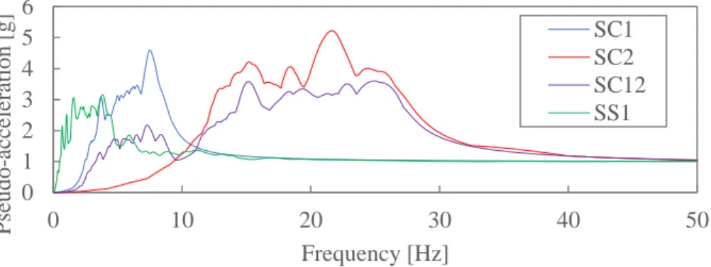
Fig. 3 – Acceleration response spectra of the dynamic input signals.

Three versions of signal SC exist: SC1 has been designed to excite only the first mode and used in the numerical study), SC2 only the second mode, SC12 being the superposition of the first two signals. Those signals are generated thanks to an inverse Fast Fourier Transformation (FFT). The SC1 spectrum is a crenel with the nominal acceleration between 0.5 times and 1.05 times the first modal frequency and equal to zero outside these bounds. This choice anticipates the modal frequency drop due to damage and allows to constantly exciting the sought modal frequency all along the test. The values of the frequencies are determined during the preliminary characterization phase (with WN, SW and HT). Increasing levels of signals are tested: 0.15 g, 0.35 g, 0.50 g, 0.90 g, 1.35 g and 1.50 g. The main objective is to detect changes in damping levels depending on new phenomena occurring with respect to the increasing peak ground acceleration (PGA). As natural seismic signal, the time evolution of the acceleration measured during the seismic event at the 3rd _{floor horizontal spectrum in} Kashiwazaki-Kariwa Nuclear Power Plant (NPP) of the Niigata-ken Chuetsu-Oki earthquake has been selected. The accelerogram and its associated acceleration response spectrum are plotted in Fig. 4 with a scale factor 2.27 in order to increase the original PGA from 0.44 g up to 1.0 g to ensure damage will occur. This signal will be labelled as SS1.

Fig. 4 – SS1 accelerogram (left) and its associated acceleration response spectrum for 5% of damping (right). 0 1 2 3 4 5 6 0 10 20 30 40 50 Pseudo -ac ce ler at ion [g ] Frequency [Hz] SC1 SC2 SC12 SS1 -1.00 -0.50 0.00 0.50 1.00 0 5 10 15 20 A cc el er at ion [g ] Time [s] 0.00 0.50 1.00 1.50 0 10 20 30 Pseudo -ac ce ler at ion [g ] Frequency [Hz]

3. Numerical study: reference model and identification

Waiting for the experimental results, a numerical model is here used as test case for the identification method. The simulation finite element code used is Cast3M [15]. In order to check the results during the experimental campaign, a robust, consistent and numerically efficient model has been considered by using multifiber beam elements associated to nonlinear constitutive material laws. Please refer to Fig. 1 andFig. 2in order to have a global view over the experimental setup and specimens.

Multifibre beam elements [16] associated with a model for concrete coupling damage and friction and taking into account unilateral effect (RICBET model [17]) and a plasticity model for steel reinforcements are able to give accurate information about damage and plasticity at the cross-section scale while ensuring a faster computer efficiency than a full three-dimensional finite elements modelling. The mesh is composed of 15 multifibre beam elements of equal length. As boundary conditions, only the rotation around z-axis is free at both supports. Due to the small displacements hypothesis, no spurious compression due to the beam shortening occurs. The mechanical parameters have been identified during standard experimental tests and modal parameters have been calibrated accordingly.

The natural seismic signal SS1 described in 2.4.2 and plotted in Fig. 3 will be used to test the identification procedure. As results, the displacements of 15 points of the beam are monitored. The first eigenfrequency of the specimen is numerically estimated at 7.63 Hz, which is slightly upper the amplification domain of the acceleration response spectrum of the natural signal (ranging from 1.0 Hz to 4.5 Hz, see Fig. 4). However, damage affecting the beam tends to decrease its first eigenfrequency, which is assumed to be progressively left-shifted towards the amplification domain and leading to the resonance of the structure

3.2 Description of the identification procedure

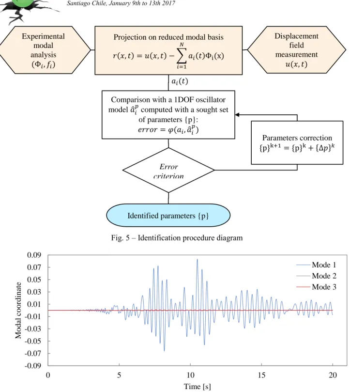
The identification procedure is performed in a two-staged (measurement/identification) optimisation routine as diagrammed in Fig. 5. To project the displacement field of the beam on a wisely chosen displacement basis (the theoretical mode shape basis Φ here), an objective function is defined in an analogous way to what is done in (Integrated) Digital Images Correlation techniques (I-DIC) such as what is detailed in [18]:

𝜂(𝑎𝑖) = ∫ (𝑢(𝑡, 𝑥) − ∑ 𝑎𝑖(𝑡)𝑓𝑖(𝑥) 𝑖 ) 2 𝑑𝑥 𝐿 0 ( 3 ) where u(t,x) is the displacement field of the beam at time t in the transverse direction, the sum term ∑ 𝑎_{𝑖 𝑖}(𝑡)𝑓_𝑖(𝑥) is the assumed decomposition on the chosen basis (the fi are the mode shape vectors while the ai are

the modal coordinates at time t) and L is the length of the beam. The minimization procedure applied on ( 3 ) leads to a linear system of equations that can be easily inverted since the size of this linear system of equations is equal to the chosen number of eigenmodes fi considered. The computation of this matrix is based on the cross scalar

products of the eigenvectors, restricted at a finite number. In practice, the first 3 eigenmodes allow representing the beam behaviour in a satisfactory way and therefore, only three wisely chosen coordinates are sufficient to express the eigenvectors. Hence, the computational cost of the projection is negligible and it can be performed on a great number of time steps. The working sampling frequency is 200 Hz and SC1 signal lasts 20.475 s, which represents 4096 time steps to process.

Fig. 5 – Identification procedure diagram

Fig. 6 – Modal projection of beam displacements for signal SS1

Following this process, the modal coordinates ai along time can be plotted as in Fig. 6. The maximum

absolute projection error is evaluated at 0.24 mm while the mean absolute projection error is estimated at 0.020 mm, which corresponds respectively to 0.29% and 0.025% of the maximum absolute displacement estimated at 84.0 mm. The following observations can be pointed out:

 the first eigenmode is, as intended, the main component of the beam response,

 the second mode remains fully inactivated,

 the third mode is slightly activated (root square mean ratio between first and third mode is 1.7%). -0.09 -0.07 -0.05 -0.03 -0.01 0.01 0.03 0.05 0.07 0.09 0 5 10 15 20 Moda l coor di nat e Time [s] Mode 1 Mode 2 Mode 3 Projection on reduced modal basis

𝑟(𝑥, 𝑡) = 𝑢(𝑥, 𝑡) − ∑ 𝑎𝑖(𝑡)Φi(x) 𝑁 𝑖=1 Error

criterion

Comparison with a 1DOF oscillator model 𝑎ො_𝑖𝑝 computed with a sought set

of parameters {p}: 𝑒𝑟𝑟𝑜𝑟 = 𝜑(𝑎𝑖, 𝑎ො𝑖

𝑝

The first and third observations are explained by the frequency content of the input signal, essentially centred on the first eigenfrequency (see Fig. 4). Moreover, the energy demand to activate higher modes increases with respect to the considered eigenfrequency. Of course, a similar explanation could be proposed for the second observation, but the first reason the second mode is not activated is due to the symmetry of the problem. Indeed, the second mode shape is geometrically anti-symmetric but, the experimental setup and the input signals are symmetric and is thus unable to initiate the imbalance required.

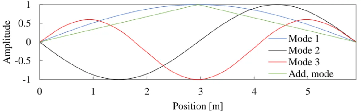
The decomposition of the beam displacements field on the standard eigenbasis leads to questions regarding its efficiency all along the loading considering the structural changes appearing aside due to damage. One solution lies in adding new vectors, which can be seen as additional degrees of freedom, in the decomposition basis in order to better describe the damaged mode shape of the beam.

Fig. 7 – Considered eigenmodes for the decomposition basis

More precisely, one possibility is to consider a triangular mode shape. This assumption is physically relevant since the mid-span is where damage initiates first and could possibly lead to the creation of a plastic hinge. Another possibility would be to consider a trapezoidal mode shape in reference to the moment diagram of the four points bending test, this case will not be studied here. This second decomposition basis leads to satisfactory results, since the maximum absolute error is reduced to 0.18 mm (versus 0.24 mm without the additional mode) and the mean of the absolute errors is 0.014 mm (versus 0.020 mm without the additional mode). Error map is a good indicator of the projection quality since it lightens up the beam areas where the displacement field is poorly approximated. Hence, it provides clues about additional deformation modes which may occur. Regarding Fig. 8 and the five higher error areas, it is clear that the enrichment of the modal basis with the fifth natural mode could improve the projection results, but the error can be considered as negligible with respect to the mid-span displacement of the beam.

Fig. 8 – Error maps (in millimetres for standard modal basis (left) and enriched modal basis (right)) Once the decomposition step is over, identification can be performed. Assuming each mode behaves as a 1 DOF oscillator and are uncoupled, it is theoretically possible to identify the dynamic properties of each oscillator. To do so, the oscillator behaviour is simulated by a Newmark’s algorithm in which the dynamic properties (i.e. the

-1 -0.5 0 0.5 1 0 1 2 3 4 5 A m pl it ude Position [m] Mode 1 Mode 2 Mode 3 Add. mode

damping ratio and the eigenfrequency) are identified through an optimisation procedure. In fact, these dynamic parameters are not identified themselves since they evolve through the test, meaning it would be necessary to operate sliding time windowing. What is done to identify the constant parameters of arbitrary chosen damping and frequency evolution laws is described below. The dynamic properties of the oscillator associated to the first mode are supposed to evolve according to the damage state of the structure.

𝑥̈(𝑡) + 2𝜉(𝐷)𝜔0(𝐷)𝑥̇(𝑡) + 𝜔02(𝐷)𝑥(𝑡) = −𝑔(𝑡) ( 4 )

In equation ( 4 ), the damping ratio ξ and the eigenmode pulsation ω0 evolve with respect to a damage index

called D. This damage index is here chosen as the one defined by [19] as detailed in equation ( 5 ). 𝐷 =𝛿𝑚 𝛿𝑦 + 𝛽∫ 𝑑𝐸 𝑡 0 𝐹𝑢𝛿𝑢 ( 5 )

In equation ( 5 ), the first term of the sum is the non-cumulative part of the index while the second one is cumulative and irreversible. δm is the maximum control displacement (here the horizontal mid-span displacement)

over the time, δy is the maximum elastic control displacement beyond which the first nonlinearities appear, and is

to identify. Fu and δu are respectively the ultimate force and control displacement capacity of the structure, the

integral term is a cumulated dissipated energy term and β is a parameter controlling the weight of the cumulative term against the non-cumulative one.

Then, the evolution law of ξ(D) is expressed in equation ( 6 ) in which two terms are summed: a constant term ξel, which is associated with the (non-material) dissipated energy observed within the elastic range of the

oscillator (when D is equal to zero) and a second term, linearly dependent on the damage index D. The evolution law of ω0 has been proposed and validated in [20].

ξ(D) = ξel + ξh.D ( 6 )

{ 𝜔 = 𝜔0 when 𝐷 < 1

𝜔0(𝐷) = (𝜔0− 𝜔𝑝)𝑒−𝑐1(𝐷−1)+ 𝜔𝑝 else

( 7 ) Once the non-linear 1 DOF oscillator fully described, an optimisation procedure is used to converge to a set of parameters solution of the equation ( 4 ): δy elastic limit control displacement; β/(Fu.δu) cumulative damage coefficient; ξel elastic damping; ξh hysteretic damping; ωp damaged pulsation; c1 frequency decreasing coefficient.

As emphasized previously, these 6 parameters have been chosen because they do not vary all along the time history analysis. The validation of the chosen models is possible through a second numerical simulation considering a different input signal. The identification error is computed in ( 8 ), where ai is the reference oscillator

displacement, y is the displacement of the identified oscillator and T is the final time of the identification time window. 𝐸 =∫ (𝑎𝑖(𝑡) − 𝑦(𝑡)) 2 𝑑𝑡 𝑇 0 ∫ 𝑎𝑖(𝑡)2𝑑𝑡 𝑇 0 ( 8 ) The oscillator movements related to the first eigenmode identified from the projection is plotted and compared with the full movement of the simulated structure in Fig. 9. Differences can be explained by the projection error (see Fig. 8), and, mostly, by the identification error.

A third identification, plotted in green in Fig. 9, is performed by assuming that the damping ratio and the natural pulsation of the oscillator do not evolve regardless of the damage state of the structure. This is equivalent to find the best elastic oscillator to fit the reference displacement. In this case, the elastic damping ratio is about

ten times the one identified in an inelastic identification since it is the only way to compensate the lack of energy dissipation of the elastic model. The high error indicator in Table 3 shows the importance to take into account changes of the dynamic properties during a high level dynamic test.

Fig. 9 – Identified oscillator behaviour

Table 3 – Comparison between elastic and inelastic identifications

Parameter Inelastic identification Elastic identification

ξel 0.02380 0.244442 ξh 0.000606 _ c1 0.077954 _ δy 0.001260 _ ωp 28.524203 _ β/(Fu.δu) 0.000008 _ Error indicator 0.1161 0.5795

4. Conclusion

The use of viscous damping to describe the energy dissipations occurring in RC structures during seismic events is still a current practice, as shown by the literature review and the design rules. However, users of such models should keep in mind that it is only a way to compute efficiently, but artificially, the resisting forces acting onto structures. The use of physical-motivated evolution laws of the damping ratios represents an alternative strategy between this artificial representation and the reality when the related parameters are appropriately chosen and identified. At the time this paper has been written, first experimental tests are to be performed soon. The experimental results should not only supply meaningful input data for the formulation of a relevant damping model taking into account several materials, structural and signal parameters but also validate the results simulated by this model through other tests using different signals and specimen. Another validation step will also be performed thanks to the database coming from the international SMART 2013 research program [12], rich of experimental data and widely simulated through different strategies.

-0.04 -0.03 -0.02 -0.01 0 0.01 0.02 0.03 0.04 0 5 10 15 20 D ispl ac em ent [ m ] Time [s] Reference Inelastic identification Elastic identification

5. Acknowledgement

The authors wish to express their most grateful thanks to CEA/DEN for its financial support. The work carried out under the SINAPS@ project has benefited from French funding managed by the National Research Agency under the program Future Investments (SINAPS@ reference No. ANR-11-RSNR-0022). The work reported in this paper has also been supported by the SEISM Institute (http://www.institut-seism.fr).

6. References

[1] Jehel P, Léger P, Ibrahimbegovic A (2014): Initial versus tangent stiffness-based Rayleigh damping in inelastic time history analysis. Earthquake Engineering & Structural Dynamics, 43, 467-484.

[2] Jacobsen, LS (1930). Steady forced vibrations as influenced by damping. Trans. ASME, 52(15), 169-181.

[3] Adhikari S, Woodhouse J (2001). Identification of damping: part 1, viscous damping. Journal of Sound and Vibration,

243(1), 43-61.

[4] Adhikari S, Woodhouse, J (2001). Identification of damping: part 2, non-viscous damping. Journal of Sound and

Vibration, 243(1), 63-88.

[5] Crambuer R, Richard B, Ile N, Ragueneau F (2013): Experimental characterization and modeling of energy dissipation in reinforced concrete beams subjected to cyclic loading. Engineering Structures, 56, 919-934.

[6] Jacobsen, LS (1960): Damping in composite structures. In Proceedings of the 2nd World Conference on Earthquake

Engineering, 2, 1029-1044.

[7] Perera R, Huerta C, Orqui JM (2008): Identification of damage in RC beams using indexes based on local modal stiffness.

Construction and Building Materials, 22 (8), 1656-1667.

[8] Franchetti P, Modena C, Feng M (2009): Nonlinear damping identification in precast prestressed reinforced concrete beams. Computer-Aided Civil and Infrastructure Engineering, 24 (8), 577-592.

[9] Carneiro J, De Melo F, Jalali S, Teixeira V, Tomás M (2006): The use of pseudo-dynamic method in the evaluation of damping characteristics in reinforced concrete beams having variable bending stiffness. Mechanics Research

Communications, 33 (5), 601-613.

[10] Demarie G et Sabia D (2011): Non-linear damping frequency identification in a progressively damaged RC element.

Experimental Mechanics, 51 (2), 229-245.

[11] Boutin C, Hans S, Ibraim E, Roussillon P (2000): In situ experiments and seismic analysis of existing buildings.

Earthquake engineering & structural dynamics, 34 (12), 1513-1529.

[12] Richard B, Fontan M, Mazars J, Voldoire F, Chaudat T, Bonfils N, Abouri S (2015): SMART 2013: Overview and lessons learnt from the international benchmark.

[13] EMSI (2016): Seismic Mechanic Studies Laboratory CEA Saclay. [Online]. Available: http://www-tamaris.cea.fr/index_en.php.

[14] AeroGo, Inc. (2016): Industry leading load bearing manufacturer. [Online]. Available: http://www.aerogo.com. [15] CEA (2016): Finite Element tool box for Structural and Fluid Mechanics. [Online]. Available:

http://www-cast3m.cea.fr/html/presentation/Plaquette_Cast3M_2015_numerique_en.pdf

[16] Davenne L, Ragueneau F, Mazars J, Imbrahimbegovic A (2003): Efficient approaches to finite element analysis in earthquake engineering. Computers & Structures, 81 (12), 1223-1239.

[17] Richard B, Ragueneau F (2013): Continuum damage mechanics based model for quasi brittle materials subjected to cyclic loadings: formulation, numerical implementation and applications. Engineering Fracture Mechanics, 98, 383-406.

[18] Hild F, Roux S, Gras R, Guerrerro N, Marante ME, Flórez-López, J (2009): Displacement measurement technique for beam kinematics. Optics and Lasers in Engineering, 47 (3), 495-503.

[19] Park YJ, Ang AHS (1985): Mechanistic seismic damage model for reinforced concrete. Journal of structural engineering.

Journal of strucural engineering, 111 (4), 722-739.

[20] Brun M (2002): Contribution à l'étude des effets endommageants des séisme proches et lointains sur des voiles en béton armé: approche simplifiée couplant la dégradation des caractéristiques dynamiques avec un indicateur de dommage, Villeurbane: INSA.