HAL Id: hal-02628753
https://hal.inrae.fr/hal-02628753
Submitted on 26 May 2020
HAL is a multi-disciplinary open access
archive for the deposit and dissemination of
sci-entific research documents, whether they are
pub-lished or not. The documents may come from
teaching and research institutions in France or
abroad, or from public or private research centers.
L’archive ouverte pluridisciplinaire HAL, est
destinée au dépôt et à la diffusion de documents
scientifiques de niveau recherche, publiés ou non,
émanant des établissements d’enseignement et de
recherche français ou étrangers, des laboratoires
publics ou privés.
Observing actual evapotranspiration from flux tower
eddy covariance measurements within a hilly watershed:
Case study of the Kamech site, Cap Bon peninsula,
Tunisia
Rim Zitouna, Laurent Prevot, Amal Chakhar, Manel Marniche-Ben Abdallah,
Frédéric Jacob
To cite this version:
Rim Zitouna, Laurent Prevot, Amal Chakhar, Manel Marniche-Ben Abdallah, Frédéric Jacob.
Ob-serving actual evapotranspiration from flux tower eddy covariance measurements within a hilly
water-shed: Case study of the Kamech site, Cap Bon peninsula, Tunisia. Atmosphere, MDPI 2018, 9 (2),
�10.3390/atmos9020068�. �hal-02628753�
atmosphere
Article
Observing Actual Evapotranspiration from Flux
Tower Eddy Covariance Measurements within a Hilly
Watershed: Case Study of the Kamech Site,
Cap Bon Peninsula, Tunisia
Rim Zitouna-Chebbi1,*ID, Laurent Prévot2, Amal Chakhar2, Manel Marniche-Ben Abdallah1,2
and Frederic Jacob1,2
1 INRGREF-LRVENC, Carthage University, BP 10 El Menzah IV, 1004 Tunis, Tunisia; manelmarniche@yahoo.fr (M.M.-B.A.); frederic.jacob@ird.fr (F.J.)
2 LISAH, Univ Montpellier, INRA, IRD, Montpellier SupAgro, F-34060 Montpellier, France; laurent.prevot@inra.fr (L.P.); chakhar.amal@gmail.com (A.C.)
* Correspondence: rimzitouna@gmail.com; Tel.: +216-98-995-497
Received: 22 December 2017; Accepted: 31 January 2018; Published: 15 February 2018
Abstract: There is a strong need for long term observations of land surface fluxes such as actual evapotranspiration (ETa). Eddy covariance (EC) method is widely used to provide ETa measurements, and several gap-filling methods have been proposed to complete inherent missing data. However, implementing gap-filling methods is questionable for EC time series collected within hilly agricultural areas at the watershed extent. Indeed, changes in wind direction induce changes in airflow inclination and footprint, and therefore possibly induce changes in the relationships on which rely gap-filling methods. This study aimed to obtain continuous ETa time series by adapting gap-filling methods to the particular conditions abovementioned. The experiment took place within an agricultural watershed in north-eastern Tunisia. A 9.6-m-high EC flux tower has been operating close to the watershed center since 2010. The sensible and latent heat fluxes data collected from 2010 to 2013 were quality controlled, and the REddyProc software was used to fill gaps at the hourly timescale. Adapting REddyProc method consisted of splitting the dataset according to wind direction, which improved the flux data at the hourly timescale, but not at the daily and monthly timescales. Finally, complete time series permitted to analyze seasonal and inter-annual variability of ETa.
Keywords:actual evapotranspiration; hilly watershed; eddy covariance; gap filling; wind direction; ORE OMERE; Tunisia
1. Introduction
In many regions of the world, water scarcity is an important issue for socio-economic development, and efficient management of water resources is required in order to ensure water and food security [1]. Actual evapotranspiration (ETa), which corresponds to the sum of soil evaporation and vegetation transpiration, is a key land surface flux that significantly drives hydrological budget [2], vegetation functioning and resulting agricultural production [3], as well as boundary layer processes and regional climate [4]. Further, ETa is strongly influenced by global change, including (1) climate forcing such as rainfall and evaporative demand and (2) anthropogenic forcing such as land use and agricultural systems [5,6]. Therefore, accurate and consistent estimates of ETa at the extent of the small watershed are required to tackle the challenges related to water resource management. Besides, such observations over the long term are mandatory for (1) diagnosing the combined effects of the involved processes (i.e., climate and anthropogenic forcing, vegetation functioning, hydrological cycle), (2) prognosticating
Atmosphere 2018, 9, 68 2 of 17
future trends by using modelling approaches based on calibration and simulation procedures [7], and (3) validating remotely sensed products [8].
To ensure accurate and continuous observations of ETa at the extent of the small watershed, the eddy covariance (EC) method is the reference technique for measuring the sensible (H) and latent (λE) heat fluxes, where λE corresponds to ETa. The EC method has been tested and proven at various spatial scales for a worldwide variety of land surface conditions, including crops, forests, snow, water bodies, urban areas, as well as mountainous and flat areas [9]. EC method has several advantages such as high temporal resolution at hourly scale and spatial integration over large areas [10]. However, EC measurements often experience large portions of missing data, as the consequence of sensor or power failures, maintenance and calibration procedures, improper weather conditions, and data rejection by quality checks [9]. Gap filling methods are therefore necessary to obtain EC based continuous time series of land surface fluxes over seasonal or inter-annual periods. In order to provide accurate estimates of H and λE when data are missing, several gap-filling methods have been proposed. These methods rely on ancillary information in time or space: the mean diurnal variation method [11], the regression method [12,13], the evaluation of two-week average Priestley–Taylor coefficient [14,15], the look-up table method [11] and the multiple imputation [16]. Most of gap filling methods were devoted to carbon dioxide measurements, for homogenous surfaces over flat or mountainous areas.
Hilly areas are widespread throughout the world. They experience intensification of rainfed agriculture, since topographical conditions permit the mobilization of water resources [17–20]. They depict strong spatial heterogeneities, due to family farming that induces very small fields. For hilly and heterogeneous cropping systems, the land surface conditions that drive ETa (i.e., radiative regime, wind and turbulence regimes, water status) can be different from those occurring within homogenous surfaces over flat/mountainous areas.
The existing gap-filling methods have not been examined over hilly cropping systems at the extent of the small watershed. This is all the more critical that these specific conditions are likely to induce different relationships between ancillary information and flux measurements, as compared to those observed for homogeneous areas over flat or mountainous terrains. When dealing with hilly cropping systems, wind direction is an important parameter. First, the combined effects of hilly topography and wind direction induced changes in airflow streamlines and turbulent fluxes [21]. At the field scale, Zitouna-Chebbi et al [22] and Zitouna-Chebbi et al [23] demonstrated the necessity to discriminate wind directions when processing EC data. Second, wind direction induces changes in the EC footprint that may subsequently spread over different patchworks of crop fields. Overall, changes in wind direction are likely to induce changes in the relationships on which rely gap-filling methods. This induces the necessity to evaluate the existing gap-filling methods, then to adapt these methods if necessary.
The current study aimed at evaluating a robust and widely used gap-filling method, for obtaining complete time series of ETa measurements over hilly cropping systems at the extent of the small watershed. We used a nearly four-years long EC measurements dataset, collected from a flux tower within an agricultural watershed. The latter was typified by hilly topography, and the footprint of the flux tower measurements integrated a patchwork of crop fields. The crops were rainfed, which minimized advection processes induced by changes in soil moisture. We evaluated the gap-filling method proposed by [24], which is widely distributed through the REddyProc package version 0.6-0. We evaluated this method on λE for ETa, but also on H that is used to estimate water status indicators (e.g., Bowen ratio, evaporative fraction). Further, including H allowed to deepen our analysis of the gap-filling method. We compared the performance of the gap-filling method when used in its original version and when adapted to the conditions of hilly and heterogeneous cropping systems, i.e., by discriminating wind directions. The performances to be compared were related to both accuracy on flux estimates and gap-filling rates, at the hourly, daily and monthly timescales. Finally, daily and monthly values of ETa were documented and analyzed in terms of temporal dynamics.
Atmosphere 2018, 9, 68 3 of 17
The paper is structured as follows. Section2present the experimental strategy (site description, experimental design, data collection and processing, implementation and evaluation of the gap-filling method), the data set to be gap-filled, and the experimental conditions with a focus on meteorology. Section 3reports the results obtained when (1) comparing of performances of the original and adapted versions of the gap-filling method; and (2) analyzing the temporal dynamics of the obtained Eta time series at the daily and monthly timescales. Conclusion discusses main outputs and future investigations.
2. Experiments 2.1. Site Description
The experiment took place within the agricultural Kamech watershed, located in the Cap Bon peninsula in north-eastern Tunisia (36◦5204000 N, 10◦5204000 E). Kamech watershed belongs to the long-term environmental research observatory OMERE (French acronym for Mediterranean Observatory of Water and the Rural Environment) that studies the impacts of anthropogenic forcing and climate change on hydrology, erosion, and water quality (http://www.umr-lisah.fr/omere). In the context of the OMERE observatory program, measuring evapotranspiration ETa at the watershed scale was recognize as a key research objective for the following reasons. On the one hand, ETa is the main component of the hydrological balance in semiarid regions, up to 80% at the yearly timescale [2]. On the other hand, ETa is rarely measured directly, and is usually estimated indirectly from the hydrological balance closure or from meteorological measurements.
The climate is Mediterranean sub-humid. Annually averaged precipitation and Penman-Monteith reference crop evapotranspiration over the 2004–2014 period are 680 mm and 1366 mm, respectively. A detailed analysis of these meteorological observations is given in Section2.5.
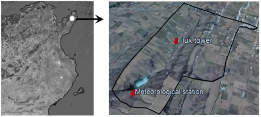
The Kamech watershed has an area of 2.45 km2. The watershed topography is globally V shaped from its middle to the outlet (Figure1), around a valley oriented from northwest to southeast. The slopes are irregular, especially on the southern rim, which has natural embankments induced by sandstone hogbacks. The altitude ranges between 94 m and 194 m above sea level (asl). The slopes range between 0% and 30%, the quartiles being 6%, 11% and 18%. The soils have sandy-loam textures, with depths ranging from 0 to 2 m according to the location within the watershed and to the local topography [17]. Most of the crops are rain-fed. They include winter cereals (durum and bread wheat, barley, oat, and triticale) and legumes (chickpeas and fava beans), which can be either harvested or grazed. The steepest parts of the watershed are covered by natural vegetation and used as rangeland for livestock. Sowing of crops starts in November and the maximum vegetation growth appears in spring, the vegetation height rarely exceeding 1 m. From the end of June (summer season) until the end of October (autumn season), the Kamech watershed is mostly under conditions of bare soil.
Atmosphere 2018, 9, x FOR PEER REVIEW 3 of 17
The paper is structured as follows. Section 2 present the experimental strategy (site description, experimental design, data collection and processing, implementation and evaluation of the gap-filling method), the data set to be gap-filled, and the experimental conditions with a focus on meteorology. Section 3 reports the results obtained when (1) comparing of performances of the original and adapted versions of the gap-filling method, and (2) analyzing the temporal dynamics of the obtained Eta time series at the daily and monthly timescales. Conclusion discusses main outputs and future investigations.
2. Experiments
2.1. Site Description
The experiment took place within the agricultural Kamech watershed, located in the Cap Bon peninsula in north-eastern Tunisia (36°52′40″ N, 10°52′40″ E). Kamech watershed belongs to the long-term environmental research observatory OMERE (French acronym for Mediterranean Observatory of Water and the Rural Environment) that studies the impacts of anthropogenic forcing and climate change on hydrology, erosion, and water quality (http://www.umr-lisah.fr/omere). In the context of the OMERE observatory program, measuring evapotranspiration ETa at the watershed scale was recognize as a key research objective for the following reasons. On the one hand, ETa is the main component of the hydrological balance in semiarid regions, up to 80% at the yearly timescale [2]. On the other hand, ETa is rarely measured directly, and is usually estimated indirectly from the hydrological balance closure or from meteorological measurements.
The climate is Mediterranean sub-humid. Annually averaged precipitation and Penman-Monteith reference crop evapotranspiration over the 2004–2014 period are 680 mm and 1366 mm, respectively. A detailed analysis of these meteorological observations is given in Section 2.5.
The Kamech watershed has an area of 2.45 km2. The watershed topography is globally V shaped from its middle to the outlet (Figure 1), around a valley oriented from northwest to southeast. The slopes are irregular, especially on the southern rim, which has natural embankments induced by sandstone hogbacks. The altitude ranges between 94 m and 194 m above sea level (asl). The slopes range between 0% and 30%, the quartiles being 6%, 11% and 18%. The soils have sandy-loam textures, with depths ranging from 0 to 2 m according to the location within the watershed and to the local topography [17]. Most of the crops are rain-fed. They include winter cereals (durum and bread wheat, barley, oat, and triticale) and legumes (chickpeas and fava beans), which can be either harvested or grazed. The steepest parts of the watershed are covered by natural vegetation and used as rangeland for livestock. Sowing of crops starts in November and the maximum vegetation growth appears in spring, the vegetation height rarely exceeding 1 m. From the end of June (summer season) until the end of October (autumn season), the Kamech watershed is mostly under conditions of bare soil.
Figure 1. The Kamech watershed. (Left) localization of the Kamech watershed within the Cap Bon
peninsula, north-eastern Tunisia. (Right) aerial map of the Kamech watershed with the localization of the flux tower and of the meteorological station.
Figure 1.The Kamech watershed. (Left) localization of the Kamech watershed within the Cap Bon peninsula, north-eastern Tunisia. (Right) aerial map of the Kamech watershed with the localization of the flux tower and of the meteorological station.
Atmosphere 2018, 9, 68 4 of 17
2.2. Experimental Design and Data Acquisition 2.2.1. Experimental Overview
The meteorological station was located at 36◦52010.500 N, 10◦5206.300 E, 108 m asl, near the catchment outlet. The measurements of ETa at the watershed scale were collected from an eddy covariance (EC) device set up on a 9.6 m-height flux tower. The flux tower was located at 36◦52039.000N, 10◦52036.400 E, 115 m asl., close to the center of the watershed (see Figure 1). In the current study, we focused on the data collected over four years (2010 to 2013). All instruments were manufacturer-calibrated and carefully checked during the experiment.
2.2.2. Meteorological Station
The meteorological station measured: (1) the solar irradiance with a SP1110 pyranometer (Skye, UK); (2) the air temperature and humidity with an HMP45C probe (Vaisala, Ventaa, Finland); (3) the wind speed with an A100R anemometer (Vector Instruments, N.Wales, UK); (4) the wind direction with a W200P wind vane (Vector Instruments, N. Wales, UK). The instruments were installed 2 m above ground (1 m for the pyranometer), following the standard of the World Meteorological Organization for agro-meteorological measurements. All sensors were connected to a CR10X data-logger (Campbell Scientific, Logan, USA). Variables were sampled at 1 Hz and stored as 30 min averages.
2.2.3. Eddy Covariance Flux Tower
Installed in march 2010, the eddy covariance (EC) tower was equipped with sensors installed at 9.6 m above the soil surface for measuring the turbulent fluxes. A three-dimensional sonic anemometer (CSAT3, Campbell Scientific, Logan, USA) measured wind speed in the three directions and air temperature at a 20 Hz frequency. The sonic anemometer was vertically set up and oriented towards North West. An open path gas H2O/CO2analyzer (LI-7500, Li-Cor Biosciences, Nebraska, USA)
measured concentrations of water vapor and CO2at a 20 Hz-frequency. A thermo-hygrometer HMP45C
sensor (Vaisala, Ventaa, Finland) measured air temperature and air humidity at a 1 Hz-frequency. All sensors were connected to a datalogger (CR3000 Campbell SC, Logan, USA) and were power supplied by photovoltaic panels connected to batteries. Data from the fast sensors (CSAT3 and LI-7500) were stored at 20 Hz frequency. Data from the slow sensor (HMP45C) were averaged over 15 min intervals. Because of experimental troubles, EC data were not collected during the last four months of 2013. Thus, the EC flux nominal dataset spread over the (March 2010–August 2013) period.
2.3. EC Flux Calculations and Quality Control 2.3.1. Calculating Convective Fluxes
The sensible heat (H) and latent (λE) heat fluxes were calculated over 30 min intervals from the sonic anemometer and the gas analyzer data, by using the ECpack library version 2.5.22 [25]. Most of the instrumental corrections proposed in the ECpack library were applied. These corrections aimed to (1) account for the distance between the sonic anemometer and the gas analyzer (2) account for the evolution of the average values over the calculation interval; (3) correct the temperature measured by the anemometer for the variations of the sound speed with air humidity; (4) correct the frequency response and path averaging; and (5) correct the mean vertical velocity (Webb term). When measuring fluxes by using the EC technique, it is conventional to rotate the sonic coordinate system. For this, we used the double rotation correction [26].
For the current study, we considered both the night-time and daytime data. The resulting 30-min flux data had a footprint of 18 ha on average, corresponding to an along-wind length of 970 m and an across-wind width of 210 m. Given the averaged field size within the experimental site was 0.5 ha, the measurement footprint integrated several crop fields. Further, the crop fields around the flux tower
Atmosphere 2018, 9, 68 5 of 17
were representative of the crop fields within the 2.45-km2size Kamech watershed (wheat, favabean, oat and rangeland).
2.3.2. Quality Control
The quality control of the 30-min flux data was performed using two standard tests that are routinely employed over flat and sloping terrains, i.e., the Steady State test and the Integral Turbulence Characteristics test. These tests permitted to ensure that the theoretical requirements for the EC measurements were fulfilled [27]. On the same site, references [22,23] applied these tests over EC datasets collected under conditions of hilly topography, and reported good energy balance closure for the selected data. We kept the high and good quality classes as defined by [28,29], since these two classes are considered as suitable for long-term observations.
2.4. The Dataset to be Gap-Filled
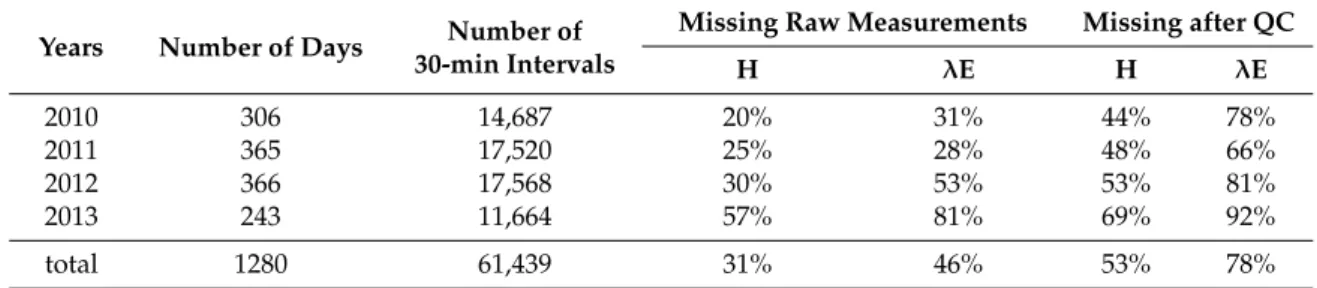
Before quality control, the rate of missing because of experimental failures (deficient energy supply, sensors malfunctioning) ranged between 20% and 57% for H, and between 28% and 81% for λE (see Table1), on a yearly basis. The rate of missing data after quality control filtering ranged between 44% and 69% for H and between 66% and 92% for λE, on a yearly basis. The rates of missing data before and after quality control filtering were similar to those reported in former studies that addressed missing data from flux tower with EC devices [30].
In terms of gap temporal distribution that might directly impacts the performances of gap filling methods, we identified 4 long periods with continuously missing data for H (from 15 December 2010 to 25 January 2011, from 24 November 2011 to 2 March 2012, and from 1 February 2013 to 30 March 2013), and for λE (from 1 May 2010 to 4 June 2010, from 15 December 2010 to 25 January 2011, from 24 November 2011 to 29 March 2012, from 10 October 2012 to 28 May 2013).
Table 1. Summary of the available flux data available before gap-filling, for the sensible (H) and latent (λE) heat fluxes. The number of 30-min intervals corresponds to the number of days of the experiment. The rates of missing data are given as percentages of the number of 30-min intervals for each year between March 2010 and August 2013. Missing raw measurements are due to experimental failures. Missing after quality control QC correspond to the sum of missing raw measurements and data eliminated by quality control (Section2.3.2).
Years Number of Days Number of 30-min Intervals
Missing Raw Measurements Missing after QC
H λE H λE 2010 306 14,687 20% 31% 44% 78% 2011 365 17,520 25% 28% 48% 66% 2012 366 17,568 30% 53% 53% 81% 2013 243 11,664 57% 81% 69% 92% total 1280 61,439 31% 46% 53% 78%
2.5. Characterization of the Meteorological Conditions
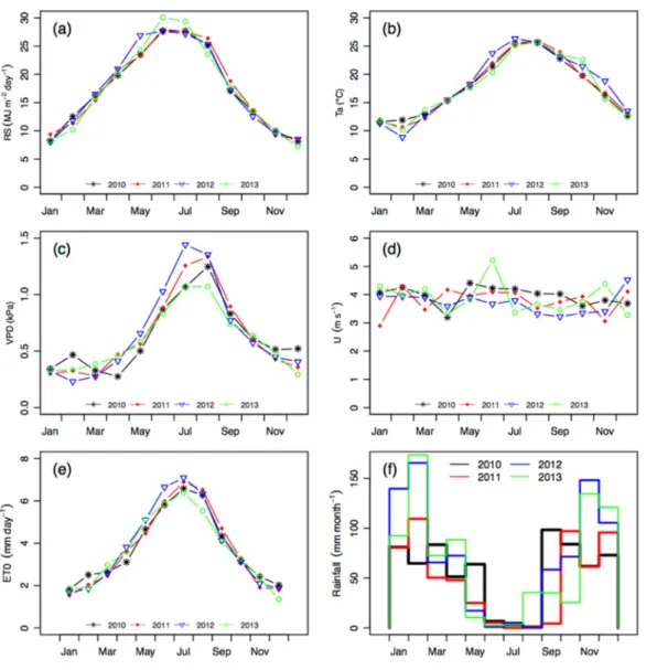
The local climatic conditions during the experiment are given in Figure2, which presents, for the four years of the experiment, the monthly average of the main climatic variables as measured by the meteorological station: solar incoming radiation, air temperature, water pressure deficit, wind speed, reference evapotranspiration and rainfall amounts. As a typical Mediterranean site [31], two contrasted periods were clearly distinguished: a relatively cold and humid period (from October to April) and a hot and dry period (from May to September). Monthly averages of solar radiation, air temperature and wind speed exhibits little inter-annual variability. Water vapor deficit inter-annual variability was larger (larger values of VPD during the summers of 2011 and 2012, lower values of VPD during the summer of 2013), which induced similar variations of the reference evapotranspiration ET0(computed
Atmosphere 2018, 9, 68 6 of 17
according to FAO-56 standard). Wind speed had a rather large averaged value, around 4 m·s−1, and did not present any seasonal variations. As usual for a Mediterranean site [32], rainfall amounts exhibited a large seasonal variability, with almost no rain during summer (June to August) and larger rainfall amounts in autumn, winter and spring. For each month, the inter-annual variability of the rainfall amounts was large, with is also commonly observed in Mediterranean areas.
Atmosphere 2018, 9, x FOR PEER REVIEW 6 of 17
averaged value, around 4 m·s−1, and did not present any seasonal variations. As usual for a
Mediterranean site [32], rainfall amounts exhibited a large seasonal variability, with almost no rain during summer (June to August) and larger rainfall amounts in autumn, winter and spring. For each month, the inter-annual variability of the rainfall amounts was large, with is also commonly observed in Mediterranean areas.
Figure 2. Climatic conditions during the four years of the experiment, recorded at the
meteorological station: (a) Incoming solar radiation; (b) air temperature; (c) water vapor deficit; (d) wind speed; (e) reference evapotranspiration; (f) rainfall amounts. Values in (a) to (e) are the monthly averages, values in (f) are cumulated rainfall amounts.
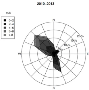
Figure 3 shows the wind rose deduced from wind speeds and directions that were recorded by the meteorological station at the hourly timescale. As no systematic seasonal variation of the wind direction was observed, Figure 3 covers the four years of the experiment. Two dominant wind directions were clearly distinguished: a north-western sector, with winds coming from directions between southwest (220°) and east-northeast (70°) directions (clockwise degrees, north is 0°) and a southern sector, with winds coming from the other directions. These two sectors will be hereafter referred to as NW and S, respectively. The NW winds were more frequent (66%) than the S winds (34%). Even if the variability of wind speeds was low at the monthly time scales (see Figure 2), we could observe large speed values at hourly time scale, larger than 8 m·s−1, especially for NW winds.
Figure 2.Climatic conditions during the four years of the experiment, recorded at the meteorological station: (a) Incoming solar radiation; (b) air temperature; (c) water vapor deficit; (d) wind speed; (e) reference evapotranspiration; (f) rainfall amounts. Values in (a) to (e) are the monthly averages, values in (f) are cumulated rainfall amounts.
Figure3shows the wind rose deduced from wind speeds and directions that were recorded by the meteorological station at the hourly timescale. As no systematic seasonal variation of the wind direction was observed, Figure3covers the four years of the experiment. Two dominant wind directions were clearly distinguished: a north-western sector, with winds coming from directions between southwest (220◦) and east-northeast (70◦) directions (clockwise degrees, north is 0◦) and a southern sector, with winds coming from the other directions. These two sectors will be hereafter referred to as NW and S, respectively. The NW winds were more frequent (66%) than the S winds (34%). Even if the variability of wind speeds was low at the monthly time scales (see Figure2), we could observe large speed values at hourly time scale, larger than 8 m·s−1, especially for NW winds.
Atmosphere 2018, 9, 68 7 of 17
Atmosphere 2018, 9, x FOR PEER REVIEW 7 of 17
Figure 3. Distribution of the wind directions throughout the four years experiment. The wind rose
indicates the occurrence of wind speeds for 16 wind directions.
2.6. Method for Gap Filling EC Data 2.6.1. REddyProc Gap Filling Method
In this study, the gap filling method proposed by [24] was chosen. This choice was motivated by the following reasons. First, this method was tested and proven for a worldwide variety of land surface conditions, since it was adopted by the global network of micrometeorological measurement sites FLUXNET (http://fluxnet.fluxdata.org/) as a standardized method [33,34]. Second, this method does not involve much ancillary information, since it only requires meteorological data. Third, this method is world-widely spread through the R package labelled REddyProc that was developed by [24] at the Max Planck Institute for Biogeochemistry.
This package relies on a gap-filling technique similar to that proposed by [11], and additionally includes (1) the co-variation of fluxes with meteorological variables, and (2) the temporal auto-correlation of the fluxes. In this method, three different conditions are successively processed within an iterative procedure [24]:
• Step 1: All meteorological data of interest are available (solar incoming radiation Rs, air
temperature Ta, and vapor pressure deficit VPD). The missing values of H or λE are replaced by the averaged values obtained under similar meteorological conditions for a given time window. Similar meteorological conditions correspond to Rs, Ta and VPD values that do not deviate by more than 50 W·m−2, 2.5 °C, 0.5 kPa, respectively. If no similar meteorological conditions are
present within a 14-day time window centered on the date of interest, the time window is extended to 28 days.
• Step 2: Rs only is available. The same approach is taken, and similar meteorological conditions correspond to Rs values that does not deviate by more than 50 W·m−2. The time window is 14
days centered on the date of interest.
• Step 3: All meteorological data are missing. The missing value of H or λE are replaced by values derived at the same time of the day from a mean diurnal course (MDC). The latter are computed on the date of interest when possible, or from the two adjacent days otherwise.
If after these three first steps any value cannot be filled, the three steps are repeated with a 7 days incremental increase of the window size, until the value can be filled. The iterative procedure is stopped when no replacement value is found in a 280 days window.
Figure 3.Distribution of the wind directions throughout the four years experiment. The wind rose indicates the occurrence of wind speeds for 16 wind directions.
2.6. Method for Gap Filling EC Data 2.6.1. REddyProc Gap Filling Method
In this study, the gap filling method proposed by [24] was chosen. This choice was motivated by the following reasons. First, this method was tested and proven for a worldwide variety of land surface conditions, since it was adopted by the global network of micrometeorological measurement sites FLUXNET (http://fluxnet.fluxdata.org/) as a standardized method [33,34]. Second, this method does not involve much ancillary information, since it only requires meteorological data. Third, this method is world-widely spread through the R package labelled REddyProc that was developed by [24] at the Max Planck Institute for Biogeochemistry.
This package relies on a gap-filling technique similar to that proposed by [11], and additionally includes (1) the co-variation of fluxes with meteorological variables, and (2) the temporal auto-correlation of the fluxes. In this method, three different conditions are successively processed within an iterative procedure [24]:
• Step 1: All meteorological data of interest are available (solar incoming radiation Rs, air temperature Ta, and vapor pressure deficit VPD). The missing values of H or λE are replaced by the averaged values obtained under similar meteorological conditions for a given time window. Similar meteorological conditions correspond to Rs, Ta and VPD values that do not deviate by more than 50 W·m−2, 2.5◦C, 0.5 kPa, respectively. If no similar meteorological conditions are present within a 14-day time window centered on the date of interest, the time window is extended to 28 days.
• Step 2: Rs only is available. The same approach is taken, and similar meteorological conditions correspond to Rs values that does not deviate by more than 50 W·m−2. The time window is 14 days centered on the date of interest.
• Step 3: All meteorological data are missing. The missing value of H or λE are replaced by values derived at the same time of the day from a mean diurnal course (MDC). The latter are computed on the date of interest when possible, or from the two adjacent days otherwise.
If after these three first steps any value cannot be filled, the three steps are repeated with a 7 days incremental increase of the window size, until the value can be filled. The iterative procedure is stopped when no replacement value is found in a 280 days window.
Atmosphere 2018, 9, 68 8 of 17
2.6.2. Adapting the REddyProc Method to Hilly Cropping Systems
REddyProc was applied to fill gaps within incomplete time series of H and λE measurements, labelled HORIand λEORIhereafter, by using the meteorological data collected at the local meteorological
station: global radiation, air temperature and vapor pressure deficit. The time series of H and λE measurements to be completed were quality controlled data (see Section2.3.2).
• First, REddyProc was applied in its original version without discriminating the two dominant wind directions (classical way). The obtained gap-filled data were labelled HREPand λEREP.
• Second, REddyProc was applied after splitting the data according to the two main wind directions, i.e., north-west (NW) and south (S). We split the complete time series into two datasets. The NW (respectively S) dataset included the HORIand λEORIdata collected under NW (respectively S)
wind conditions. REddyProc was applied over each of these two datasets. The resulting gap-filled datasets were finally merged. The obtained energy fluxes were labelled HRNSand λERNS.
2.6.3. Cross-Validation of REddyProc: Artificial Gaps
Splitting the initial time series of quality controlled data into two datasets for north-western and southern winds induced the removal of 34% and 66% for the NW and S datasets, respectively (see Section 2.5). In order to quantify the resulting deterioration on the REddyProc gap-filling performances, we introduced artificial gaps in the initial time series, to which we applied the REddyProc procedure. We then compared the gap-filled data against the initial values [10,35]. Conducting this cross-validation analysis also permitted to quantify the REddyProc gap filling performances for the specific conditions of the study area. Creating artificial gaps consisted of randomly removing part of the existing dataset. We removed 10% to 70% data from the original time series, with a 10% step.
Given the initial time series already contained gaps because of instrumental malfunctioning or quality control filtering, we selected a part of the time series that included a large number of data, so that it was possible to remove up to 70% of the existing data. This selected part of the time series spread from 9 February to 15 September 2011. REddyProc was applied on the artificially gapped time series, and we compared the estimated H and λE fluxes against their initial values, using standard statistical indicators (absolute and relative bias, absolute and relative root mean square error RMSE, coefficient of determination R2).
3. Results
3.1. Cross-Validation of REddyProc
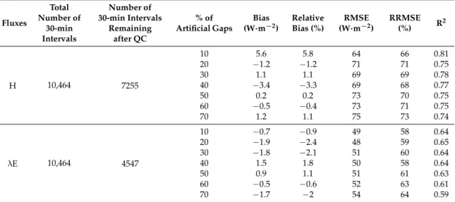
The cross-validation of the REddyProc gap-filling procedure is presented in Table2. Over the considered period, 9 February to 15 September 2011 (10,464 30-min intervals), the number of 30-min intervals flux data remaining after quality control were 7255 (69%) and 4547 (43%) for H and λE, respectively. The number of artificial gaps introduced varied between 725 and 5078 (10% and 70% of the remaining data) for H, and between 454 and 3182 (10% and 70% of the remaining data) for λE. The artificial gaps introduced in this cross-validation analysis were adding to the already missing flux data (sixth and seventh columns of Table1), leading to larger percentages of actually missing flux data: between 38% and 79% for H and between 61% and 87% for λE.
The flux magnitudes were not affected by the random sampling of artificial gaps, since the average values ranged between 97 and 104 W·m−2for H, and between 81 and 86 W·m−2for λE. Regardless of artificial gap rate, the bias between the initial and the estimated fluxes was very low: between−3.4 and 5.6 W·m−2for H, and between−1.9 and 1.5 W·m−2for λE. The RMSE of the estimation increased slightly with the rate of artificial gaps: from 64 to 75 W·m−2for H, and from 49 to 54 W·m−2for λE. Accordingly, the corresponding R2decreased slightly with the increasing rate of artificial gaps.
Atmosphere 2018, 9, 68 9 of 17
Table 2. Statistical indicators for the cross-validation of REddyProc. The total number of 30-min intervals correspond to the duration of the considered period (9 February 2011 to 15 September 2011). The percentage of artificial gaps was applied to the number of 30-min intervals remaining after QC. Accuracy is quantified using statistical indicators (absolute and relative bias, absolute and relative RMSE, coefficient of determination R2).
Fluxes Total Number of 30-min Intervals Number of 30-min Intervals Remaining after QC % of Artificial Gaps Bias (W·m−2) Relative Bias (%) RMSE (W·m−2) RRMSE (%) R 2 H 10,464 7255 10 5.6 5.8 64 66 0.81 20 −1.2 −1.2 71 71 0.75 30 1.1 1.1 69 69 0.78 40 −3.4 −3.3 69 68 0.77 50 0.2 0.2 73 70 0.75 60 −0.5 −0.4 73 71 0.75 70 1.2 1.1 75 73 0.74 λE 10,464 4547 10 −0.7 −0.9 49 58 0.64 20 −1.9 −2.4 48 59 0.65 30 −1.8 −2.1 51 60 0.64 40 1.5 1.8 50 58 0.64 50 0.9 1.1 51 61 0.63 60 −0.5 −0.6 52 63 0.61 70 −1.7 −2 54 64 0.59 3.2. Application of REddyProc
3.2.1. Impact of Discriminating Wind Directions with REddyProc
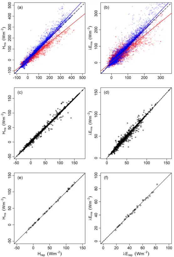
Figure4presents the comparison of the sensible and latent heat fluxes estimated by REddyProc if splitting (RNS) or not (REP) the H and λE datasets according to wind direction. Figure4displays results at the hourly, daily and monthly timescales. We recall wind direction are labelled NW for north-western winds and S for southern winds.
At the hourly timescale and for NW winds, the sensible heat flux estimates HREP and HRNS
were very similar, with a regression line close to the 1:1 line (slope = 1.07, intercept = 1.9), and a small dispersion (RMSE = 11.0 W·m−2). Conversely, under S winds, applying REddyProc without discriminating the wind directions (HREP) distinctly overestimated the sensible heat flux estimates
(HRNS) obtained when discriminating wind directions (slope = 0.81, intercept =−1.9), with a slightly
larger dispersion (RMSE = 15.7 W·m−2). Very similar results were obtained for the latent heat flux estimates: λEREPand λERNSwere very close under NW winds (slope = 1.05, intercept =−0.5),
with a small dispersion (RMSE = 12.2 W·m−2), whereas λEREPoverestimated λERNSunder S winds
(slope = 0.81, intercept = 3.8), with a slightly larger dispersion (RMSE = 18.9 W·m−2).
For H and λE daily flux data obtained by integrating hourly values at the daily timescale (average of the 48 half-hourly fluxes, from 00:00 to 24:00), we obtained very similar results when considering REddyProc gap-filled time series with (RNS) or without (REP) discrimination of wind directions (see Figure4). Indeed, the regression lines between RNS and REP flux estimates were very close to the 1:1 line, and the corresponding RMSE values (4.5 and 4.6 W·m−2for H and λE, respectively), were lower than those obtained at the hourly timescale.
Further, the daily flux data were integrated at the monthly time scale. As expected, we did not observe any difference, for both H and λE, when considering REddyProc gap-filled time series with or without discrimination of wind directions (REP vs. RNS). The dispersion around the regression line was low, 1.3 and 1.7 W·m−2for H and λE, respectively.
Atmosphere 2018, 9, 68 10 of 17
Atmosphere 2018, 9, x FOR PEER REVIEW 10 of 17
Figure 4. Comparison of the fluxes estimated by REddyProc if splitting (label RNS) or not (label
REP) the H and λE datasets according to wind direction (NW for north-western winds and S for southern wind). Left column: sensible heat fluxes (H); right column: latent heat fluxes (λE). First line: (a) H hourly fluxes (30-min intervals); (b) λE hourly fluxes; fluxes under NW winds are in blue; fluxes under S winds are in red. Second line: (c) H fluxes integrated at daily time scale; (d) λE fluxes integrated at daily time scale; third line: (e) H fluxes integrated at monthly time scale, (f) λE. fluxes integrated at monthly time scale. Continuous lines: regression line; dashed lines: 1:1 lines.
3.2.2. Gap Filling Rates
The percentages of missing data remaining after application of REddyProc are given in the four last columns of Table 3, for both ways of applying REddyProc (REP and RNS). REddyProc was able
Figure 4. Comparison of the fluxes estimated by REddyProc if splitting (label RNS) or not (label REP) the H and λE datasets according to wind direction (NW for north-western winds and S for southern wind). Left column: sensible heat fluxes (H); right column: latent heat fluxes (λE). First line: (a) H hourly fluxes (30-min intervals); (b) λE hourly fluxes; fluxes under NW winds are in blue; fluxes under S winds are in red. Second line: (c) H fluxes integrated at daily time scale; (d) λE fluxes integrated at daily time scale; third line: (e) H fluxes integrated at monthly time scale, (f) λE. fluxes integrated at monthly time scale. Continuous lines: regression line; dashed lines: 1:1 lines.
Atmosphere 2018, 9, 68 11 of 17
3.2.2. Gap Filling Rates
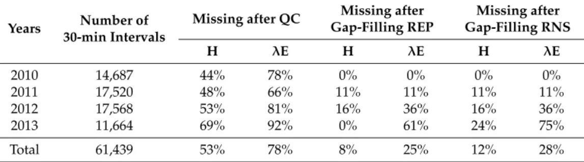
The percentages of missing data remaining after application of REddyProc are given in the four last columns of Table3, for both ways of applying REddyProc (REP and RNS). REddyProc was able to fill gaps most of the time, except when periods with missing data lasted too long. We observed different results from one year to another, because of different periods with flux tower malfunctions. 1. In May and June 2010, the LI-7500 analyzer experienced a 34 days-long failure without λE
measurements. REddyProc was able to fill all the missing λE data.
2. In December 2010 and January 2011, the flux tower experienced a 41 days-long failure without H and λE measurements. REddyProc was able to fill all the missing H and λE data.
3. From November 2011 to March 2012, the flux tower experienced several failures, without H and λE measurements for 99 and 126 days, respectively. Gap-filling for missing data was only partial, leading to a 99-day period without final data for both H and λE.
4. From October 2012 to May 2013, the flux tower experienced several failures, without H and λE measurements for 57 and 224 days, respectively. REddyProc was able to fill all the missing H data, but λE times series were not gap-filled during 221 days on 224.
Finally, the way of applying REddyProc, without (REP) or with (RNS) separating the wind directions, had no influence on the rate of gap-filled data (see Table1), except in 2013.
Table 3.Summary of the available flux data available before and after gap-filling, for the sensible (H) and latent (λE) heat fluxes. The number of 30-min intervals correspond to the number of days of the experiment. The rates of missing data are given as percentages of the number of 30-min intervals for each year. Missing after QC correspond to the sum of missing raw measurements and data eliminated by quality control (Section2.3.2). Missing data after gap-filling are given for both way of applying REddyProc ore (REP): before separating wind directions, and (RNS) after splitting. (see Section2.6.2).
Years Number of 30-min Intervals
Missing after QC Missing after Gap-Filling REP Missing after Gap-Filling RNS H λE H λE H λE 2010 14,687 44% 78% 0% 0% 0% 0% 2011 17,520 48% 66% 11% 11% 11% 11% 2012 17,568 53% 81% 16% 36% 16% 36% 2013 11,664 69% 92% 0% 61% 24% 75% Total 61,439 53% 78% 8% 25% 12% 28%
3.3. Seasonal Variations of Daily Surface Fluxes
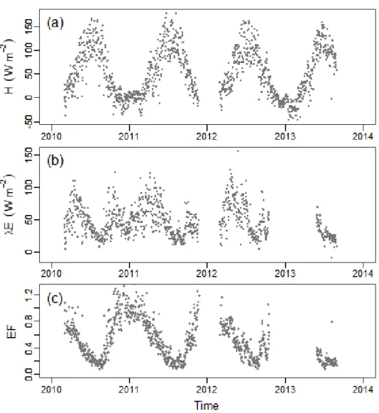
The seasonal evolution of the sensible (H) and the latent (λE) heat fluxes, at the daily timescale, is presented on Figure 5, along with the evolution of the evaporative fraction EF, evaluated as EF = λE/(H + λE). Both H and λE fluxes in Figure5were gap-filled by REddyProc without discriminating the wind directions (REP), since such discrimination had no impact at the daily timescale.
The daily values of sensible heat flux H exhibited a regular evolution over the seasons, with maximum values around 170 W·m−2in summer (June to August), and minimum values in winter (November to February). Negative values of the sensible heat flux could be observed during winter, down to−50 W·m−2. The daily values of latent heat flux λE increased from winter to spring, reaching its maximum in April, around 120 W·m−2, which correspond to 3.5 mm·day−1. The latent heat flux decreased rapidly from the end of spring to summer, reaching very low values in August, down to 15 W·m−2 (0.5 mm·day−1). The latent heat flux increased in fall (around 80 W·m−2), and then decreased during winter (around 40 W·m−2).
Atmosphere 2018, 9, 68 12 of 17
The seasonal evolution of the evaporative fraction EF was rather regular, with low values, between 0.1 and 0.2, during summer, and with large values, between 0.8 and 1.2, during winter, the EF values exceeding unity corresponding to the periods during which the sensible heat flux was negative.
Atmosphere 2018, 9, x FOR PEER REVIEW 12 of 17
Figure 5. Seasonal evolution of the land surface fluxes at the daily timescale. (a) Sensible heat flux
(H); (b) Latent heat fluxes (λE); (c) Evaporative fraction (EF).
3.4. Monthly Evapotranspiration
Daily latent heat fluxes λE were monthly averaged, which permitted to reduce the day-to-day variability observed at the daily time scale, and next converted in actual evapotranspiration units (mm·day−1). Figure 6 presents the seasonal evolution of actual evapotranspiration (ETa) and of its
ratio to reference evapotranspiration ET0, the latter being deduced from measurements at the
meteorological station (see Section 2.5). Actual evapotranspiration ETa followed a classical behaviour for Mediterranean rainfed crops, increasing from 1–1.5 mm·day−1 in winter to 2.5–3
mm·day−1 in April. From the end of spring to summer, ETa regularly decreased, reaching a
minimum below 1 mm·day−1 in August. During fall, ETa increased again, as a consequence of
rainfall events that are usual during that part of the year, then decreased in winter, as a consequence of the decrease of the reference evapotranspiration.
Figure 5.Seasonal evolution of the land surface fluxes at the daily timescale. (a) Sensible heat flux (H); (b) Latent heat fluxes (λE); (c) Evaporative fraction (EF).
3.4. Monthly Evapotranspiration
Daily latent heat fluxes λE were monthly averaged, which permitted to reduce the day-to-day variability observed at the daily time scale, and next converted in actual evapotranspiration units (mm·day−1). Figure 6presents the seasonal evolution of actual evapotranspiration (ETa) and of its ratio to reference evapotranspiration ET0, the latter being deduced from measurements at the
meteorological station (see Section2.5). Actual evapotranspiration ETa followed a classical behaviour for Mediterranean rainfed crops, increasing from 1–1.5 mm·day−1in winter to 2.5–3 mm·day−1in April. From the end of spring to summer, ETa regularly decreased, reaching a minimum below 1 mm·day−1in August. During fall, ETa increased again, as a consequence of rainfall events that are usual during that part of the year, then decreased in winter, as a consequence of the decrease of the reference evapotranspiration.
Atmosphere 2018, 9, 68 13 of 17
Atmosphere 2018, 9, x FOR PEER REVIEW 13 of 17
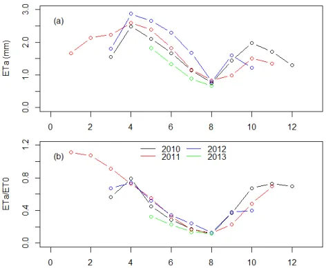
Figure 6. Seasonal evolution of the actual evapotranspiration at monthly time scale, during the four
years of the experiment. (a) Actual evapotranspiration (ETa); (b) Ratio of actual evapotranspiration to reference evapotranspiration ET0.
Inter-annual difference between monthly ETa was larger in spring and autumn, and it was lowest in summer. To remove the influence of inter-annual variability of climatic demand on that of ETa, we also addressed the ratio of ETa/ET0. As an example, the actual evapotranspiration was slightly larger in May 2012 than in May 2013, despite reference evapotranspiration rates were almost equal. Then, the inter-annual variability of the ETa/ET0 ratio was lower than that observed for ETa, and it was negligible in (i) April and June in 2011 and 2012, and (ii) November 2010 and 2011.
4. Discussion
The results obtained when cross-validating REddyProc confirmed that the latter was able to provide un-biased and acceptable estimates of missing flux data, even for large rates of missing data (see Table 2). The REddyProc appeared to be robust when facing large gap rates, as we observed a slight increase of relative RMSE values as gap rates largely increased. This was an important outcome, since adapting REddyProc to hilly cropping systems at the extent of the small watershed was likely to induce larger gap rates because of splitting the H and λE dataset according to wind direction. Finally, the RMSE values obtained were slightly better than those reported by [10] who obtained values between 20% and 150% for an artificial gap rate of 20% with λE daytime conditions and different gap filling methods.
When comparing REddyProc retrievals with and without discrimination of wind directions, the obtaining of very different H and λE flux values for southern winds underlined the need to conduct such discrimination at the hourly timescale. This was ascribed to the prevalent replacement of missing flux data under southern (S) winds by flux data under north-western (NW) winds when applying REddyProc without discrimination of wind directions, since NW wind were more frequent that S winds in the original dataset (66% versus 33%, see Section 2.5). Further, this is consistent with former studies that reported the need to discriminate wind directions when processing EC measurements in similar conditions [22,23]. At the daily timescale, we observed very small differences between REddyProc retrievals with and without discrimination of wind directions. This was ascribed to three reasons. First, fluxes obtained at the daily timescale integrated both REddyProc gap-filled values and actual values, where the latter did not vary when applying
Figure 6.Seasonal evolution of the actual evapotranspiration at monthly time scale, during the four years of the experiment. (a) Actual evapotranspiration (ETa); (b) Ratio of actual evapotranspiration to reference evapotranspiration ET0.
Inter-annual difference between monthly ETa was larger in spring and autumn, and it was lowest in summer. To remove the influence of inter-annual variability of climatic demand on that of ETa, we also addressed the ratio of ETa/ET0. As an example, the actual evapotranspiration was slightly larger in May 2012 than in May 2013, despite reference evapotranspiration rates were almost equal. Then, the inter-annual variability of the ETa/ET0 ratio was lower than that observed for ETa, and it was negligible in (i) April and June in 2011 and 2012, and (ii) November 2010 and 2011.
4. Discussion
The results obtained when cross-validating REddyProc confirmed that the latter was able to provide un-biased and acceptable estimates of missing flux data, even for large rates of missing data (see Table2). The REddyProc appeared to be robust when facing large gap rates, as we observed a slight increase of relative RMSE values as gap rates largely increased. This was an important outcome, since adapting REddyProc to hilly cropping systems at the extent of the small watershed was likely to induce larger gap rates because of splitting the H and λE dataset according to wind direction. Finally, the RMSE values obtained were slightly better than those reported by [10] who obtained values between 20% and 150% for an artificial gap rate of 20% with λE daytime conditions and different gap filling methods.
When comparing REddyProc retrievals with and without discrimination of wind directions, the obtaining of very different H and λE flux values for southern winds underlined the need to conduct such discrimination at the hourly timescale. This was ascribed to the prevalent replacement of missing flux data under southern (S) winds by flux data under north-western (NW) winds when applying REddyProc without discrimination of wind directions, since NW wind were more frequent that S winds in the original dataset (66% versus 33%, see Section2.5). Further, this is consistent with former studies that reported the need to discriminate wind directions when processing EC measurements in similar conditions [22,23]. At the daily timescale, we observed very small differences between REddyProc retrievals with and without discrimination of wind directions. This was ascribed to three
Atmosphere 2018, 9, 68 14 of 17
reasons. First, fluxes obtained at the daily timescale integrated both REddyProc gap-filled values and actual values, where the latter did not vary when applying REddyProc with or without discrimination of wind directions. Second, under NW wind directions that were dominant (66%), applying REddyProc with or without discrimination of wind directions led to very similar estimates of the fluxes at hourly time scale (see Figure4). Third, the difference between the two methods was proportional to the magnitude of the convective fluxes (see Figure4). Thus, integrating the fluxes at the daily timescale decreased the difference between the two methods, as large magnitude fluxes around noon were averaged with (1) low magnitude fluxes around early morning and late afternoon, and (2) night-time negative fluxes. Finally, we could not compare our results with former studies, because we did not find any literature report on this issue.
Applying REddyProc with or without discrimination of wind directions had no influence on the rate of gap-filled data, except in 2013 for which a failure of the wind wane at the meteorological station occurred concurrently to the failure of the flux tower. In this case, the concurrent failures prevented the application of the REddyProc with discrimination of wind directions, whereas it was possible to apply the REddyProc without discrimination of wind directions. Overall, REddyProc was able to find H and λE data with similar meteorological conditions, but difference in convective fluxes for similar meteorological conditions were likely to occur because of lack of a soil moisture proxy in the REddyProc method. Finally, the gap filling rate we obtained for H (between 65% and 100% of missing data) and λE (between 20% and 100%), could not be compared to outcomes from literature, owing to the lack of reports on this issue.
The sensible and the latent heat fluxes, as well as the evaporative fraction, exhibited large day-to-day variability, that could be ascribed to the variability of meteorological conditions, including rainfall events that might induce an increase of the latent heat flux during the next days. The seasonal dynamics we observed for the daily values of sensible of heat flux H were mainly driven by the temporal evolution of incoming solar radiation and air temperature. The maximum values we observed in April for latent heat flux λE were ascribed to the combined effects of vegetation growth, soil moisture availability, and intermediate values of reference evapotranspiration. The rapid decrease in latent heat flux E from the end of spring to summer was explained by vegetation maturation and next bare soil that combined with rainfall decrease. Finally, the latent heat flux increased in fall with the start of the rainy season, and then decreased during winter with the decrease of the reference evapotranspiration. In terms of flux magnitude, [36] reported similar monthly values from scintillometer measurements within the same study area during spring (April–June) and summer (June–July) 2006, with values of 2.3 mm·day−1and 0.5 mm·day−1, respectively.
Inter-annual differences between monthly ETa were larger in spring and autumn, which was explained by the larger inter-annual variability in rainfalls for these periods of the year. In contrast, a lower inter-annual variability in ETa was observed in summer since rainfalls were negligible for this period. Subsequently to removing the influence of climatic demand, the inter-annual variability of the ratio ETa/ET0 was smaller than that observed for ETa. This ratio was very sensitive to the rainfall amounts during the fall, with an increase of ETa/ET0arising sooner during the wet September months
of 2010 and 2012 than during the dry September month of 2011. Finally, The ETa/ET0values reported
here were lower than 1.2, and therefore were within the confidence interval proposed by Allen [37]. Also, the ETa/ET0summer values (0.15 on average) were close to the Kc value proposed by FAO
(The Food and Agriculture Organization) 56 [38] for bare soils (i.e., Kcini for winter wheat). 5. Conclusions
The main outcomes of the current study are the following. First, the REddyProc method is robust when facing large rates of missing data to be filled. This is of importance when the dataset to be filled have to be split in accordance to different land surface conditions, wind direction in our case. This is also of importance since REddyProc relies on meteorological data that are usually collected along with EC measurement. Second, it appears to be necessary to discriminate wind directions when filling
Atmosphere 2018, 9, 68 15 of 17
gaps within time series of land surface convective fluxes at the hourly timescale, in the context of hilly cropping systems at the extent of small watershed. This is consistent with former studies that reported the need to discriminate wind directions when processing EC measurements in similar conditions.
Future works should address the aforementioned issues by considering other gap-filling methods that rely on different ancillary information (i.e., rain or soil moisture that is a key driver of land surface evapotranspiration or evaporative fraction when latent heat flux λE data are missing and sensible heat flux H data are available). Also, our results gave great confidence in the observation of land surface fluxes by EC measurements over hilly cropping systems at the extent of small watershed. Then, the obtaining of complete time series for evapotranspiration at the extent of the small watershed opens the path for (1) cross-analysing these time series along with those of other components of the hydrological budget and (2) cross-analysing these times series along with trends in land use and climate forcing. Acknowledgments:The author’s express their thanks to (1) the Environmental Research Observatory OMERE (http://www.obs-omere.org) which policy drives the availability of the data used in the current study (https:// zenodo.org/record/821527#.WVZcssbpORs); (2) the MISTRALS / SICMED Lebna project and the French National Research Agency (ANR) TRANSMED ALMIRA project (contract ANR-12-TMED-0003) for their financial support; as well (3) the technical staff from INRGREF and UMR LISAH, particularly Rim Louati and François Garnier.
Author Contributions: R.Z.-C. and L.P. conceived and designed the experiments; R.Z.-C. performed the experiments; A.C. and M.M.-B.A. analysed the data; L.P., R.Z.-C. and A.C. contributed to result analysis; R.Z.-C., L.P. and F.J. wrote the paper.
Conflicts of Interest:The authors declare no conflict of interest. The founding sponsors had no role in the design of the study; in the collection, analyses, or interpretation of data; in the writing of the manuscript, and in the decision to publish the results.
References
1. Besbes, M.; Chahed, J.; Hamdane, A. Sécurité Hydrique de la Tunisie (Water Security of Tunisia); De Marsily, G., Ed.; Éditions L’Harmattan: Paris, France, 2014.
2. Moussa, R.; Chahinian, N.; Bocquillon, C. Distributed hydrological modelling of a Mediterranean mountainous catchment—Model construction and multi-site validation. J. Hydrol. 2007, 337, 35–51. [CrossRef]
3. Steduto, P.; Hsiao, T.C.; Raes, D.; Fereres, E. AquaCrop—The FAO crop model tosimulate yield response to water: I. Concepts and underlying principles. Agron. J. 2009, 101, 426–437. [CrossRef]
4. Wang, K.C.; Dickinson, R.E. A review of global terrestrial evapotranspiration: Observation, modeling, climatology, and climatic variability. Rev. Geophys. 2012, 50. [CrossRef]
5. Seneviratne, S.I.; Corti, T.; Davin, L.E.; Hirschi, M.; Jaeger, E.B.; Lehner, I.; Orlowsky, B.; Teuling, A.J. Investigating soil moisture–climate interactions in a changing climate: A review. Earth Sci. Rev. 2010, 99, 125–161. [CrossRef]
6. Cai, X.; Zhang, X.; Noël, P.H.; Shafiee-Jood, M. Impacts of climate change on agricultural water management: A review. WIREs Water 2015, 2, 439–455. [CrossRef]
7. Li, Q.; Ishidaira, H. Development of a biosphere hydrological model considering vegetation dynamics and its evaluation at basin scale under climate change. J. Hydrol. 2012, 412, 3–13. [CrossRef]
8. Karimi, P.; Bastiaanssen, W.G.M. Spatial evapotranspiration, rainfall and land use data in water accounting—Part 1: Review of the accuracy of the remote sensing data. Hydrol. Earth Syst. Sci. 2015, 19, 507–532. [CrossRef]
9. Aubinet, M.; Vesala, T.; Papale, D. Eddy Covariance. In A Practical Guide to Measurement and Data Analysis; Springer Science & Business Media: Amsterdam, The Netherlands, 2012; p. 438. [CrossRef]
10. Alavi, N.; Warland, J.S.; Berg, A.A. Filling gaps in evapotranspiration measurements for water budget studies: Evaluation of a Kalman filtering approach. Agric. For. Meteorol. 2006, 141, 57–66. [CrossRef] 11. Falge, E.; Baldocchi, D.D.; Olson, R.; Anthoni, P.; Aubinet, M.; Bernhofer, C.; Burba, G.; Ceulemans, R.;
Clement, R.; Dolman, H.; et al. Gap filling strategies for long term energy flux data sets. Agric. For. Meteorol.
2001, 107, 71–77. [CrossRef]
12. Greco, S.; Baldocchi, D.D. Seasonal variations of CO2 water vapour exchange rates over a temperate deciduous forest. Glob. Chang. Biol. 1996, 2, 183–197. [CrossRef]
Atmosphere 2018, 9, 68 16 of 17
13. Berbigier, P.; Bonnefond, J.M.; Mellmann, P. CO2and water vapour fluxes for 2 years obove Euroflux forest site. Agric. For. Meteorol. 2001, 108, 183–197. [CrossRef]
14. Wilson, K.B.; Baldocchi, D.D. Seasonal and interannual variability of energy fluxes over a broadleaved temperate deciduous forest in North America. Agric. For. Meteorol. 2000, 100, 1–18. [CrossRef]
15. Wilson, K.B.; Hanson, P.J.; Mulholland, P.J.; Baldocchi, D.D.; Wullschleger, S.D. A comparison of methods for determining forest evapotranspiration and its components: Sap-flow, soil water budget, eddy covariance and catchment water balance. Agric. For. Meteorol. 2001, 106, 153–168. [CrossRef]
16. Hui, D.; Wan, S.; Su, B.; Katul, G.; Monson, R.; Luo, Y. Gap filling missing data in eddy covariance measurements using multiple imputation (MI) for annual estimations. Agric. For. Meteorol. 2004, 121, 93–111. [CrossRef] 17. Mekki, I.; Albergel, J.; Ben Mechlia, N.; Voltz, M. Assessment of overland flow variation and blue water
production in a farmed semiarid water harvesting catchment. Phys. Chem. Earth 2006, 31, 1048–1061. [CrossRef] 18. Ameur, M.; Mtimet, N.; Khlifi, S. Effects of Small Hill Dams on Farming Systems: Bizerte Region. In Tunisia Semi-Arid Environments: Agriculture, Water Supply and Vegetation; Degenovine, K.M., Ed.; Nova Science Publishers: New York, NY, USA, 2011; pp. 159–172.
19. Joodi, N.; Satyanarayana, S.V. Design of Check Dam for Effective Utilization of the Aflaj Water Resources. Int. J. Multidiscip. Res. Dev. 2015, 2, 446–449.
20. Parimala Renganayaki, S.; Elango, L. A review on managed aquifer recharge by check dams: A case study Near Chennai, INDIA. Int. J. Res. Eng. Technol. 2013, 2, 416–423.
21. Finnigan, J.J.; Clement, R.; Malhi, Y.; Leuning, R.; Cleugh, H.A. A re-evaluation of long-term flux measurement techniques—Part 1: Averaging and coordinate rotation. Bound. Layer Meteorol. 2003, 107, 1–48. [CrossRef]
22. Zitouna-Chebbi, R.; Prévot, L.; Jacob, F.; Mougou, M.; Voltz, M. Assessing the consistency of eddy covariance measurements under conditions of sloping topography within a hilly agricultural catchment. Agric. For. Meteorol.
2012, 16, 123–135. [CrossRef]
23. Zitouna-Chebbi, R.; Prévot, L.; Jacob, F.; Voltz, M. Accounting for vegetation height and wind direction to correct eddy covariance measurements of energy fluxes over hilly crop fields. J. Geophys. Res. Atmos. 2015, 120. [CrossRef]
24. Reichstein, M.; Falge, E.; Baldocchi, D.; Papale, D.; Aubinet, M.; Berbigier, P.; Bernhofer, C.; Buchmann, N.; Gilmanov, T.; Granier, A.; et al. On the separation of net ecosystem exchange into assimilation and ecosystem respiration: Review and improved algorithm. Glob. Chang. Biol. 2005, 11, 1424–1439. [CrossRef]
25. Van Dijk, A.; Moene, A.; DeBruin, H. The Principles of Surface Flux Physics: Theory, Practice and Description of the ECPACK Library; Internal Report 2004/1; Meteorology and Air Quality Group, Wageningen University: Wageningen, The Netherlands; Available online:http://www.met.wau.nl/projects/jep/report/ecromp/
(accessed on 15 March 2011).
26. Kaimal, J.C.; Finnigan, J.J. Atmospheric Boundary Layer Flows, Their Structure and Measurement; Oxford University Press: Oxford, UK, 1994; p. 289.
27. Hiller, R.; Zeeman, M.J.; Eugster, W. Eddy-covariance flux measurements in the complex terrain of an Alpine valley in Switzerland. Bound. Layer Meteorol. 2008, 127, 449–467. [CrossRef]
28. Foken, T.; Göckede, M.; Mauder, M.; Mahrt, L.; Amiro, B.; Munger, W. Post-field data quality control. In Handbook of Micrometeorology: A Guide for Surface Flux Measurement and Analysis; Lee, X., Massman, W., Law, B., Eds.; Kluwer Academic Publishers: Dordrecht, Netherlands, 2004; pp. 181–208. [CrossRef] 29. Rebmann, C.; Göckede, M.; Foken, T.; Aubinet, M.; Aurela, M.; Berbigier, P.; Bernhofer, C.; Buchmann, N.;
Carrara, A.; Cescatti, R.C.A.; et al. Quality analysis applied on eddy covariance measurements at complex forest sites using footprint modelling. Theor. Appl. Climatol. 2005, 80, 121–141. [CrossRef]
30. Papale, D.; Reichstein, M.; Aubinet, M.; Canfora, E.; Bernhofer, C.; Kutsch, W.; Longdoz, B.; Rambal, S.; Valentini, R.; Vesala, T.; et al. Towards a standardized processing of Net Ecosystem Exchange measured with eddy covariance technique: Algorithms and uncertainty estimation. Biogeosciences 2006, 3, 571–583. [CrossRef]
31. Aschmann, H. Distribution and Peculiarity of Mediterranean Ecosystems. In Mediterranean Type Ecosystems; Chapter Part of the Ecological Studies Book Series; Springer: Berlin/Heidelberg, Germany, 1973; Volume 7, pp. 11–19.
Atmosphere 2018, 9, 68 17 of 17
33. Brilli, F.; Gioli, B.; Zona, D.; Pallozzi, E.; Zenone, T.; Fratini, G.; Calfapietra, C.; Loreto, F.; Janssens, I.A.; Ceulemans, R. Simultaneous leaf-and ecosystem-level fluxes of volatile organic compounds from a poplar-based SRC plantation. Agric. For. Meteorol. 2014, 187, 22–35. [CrossRef]
34. Horemans, J.A.; Van Gaelen, H.; Raes, D.; Zenone, T.; Ceulemans, R. Can the agricultural AquaCrop model simulate water use and yield of a poplar short-rotation coppice? GCB Bioenergy 2017, 9, 1151–1164. [CrossRef] [PubMed]
35. Zhao, X.; Huang, Y. A comparison of three gap filling techniques for eddy covariance net carbon fluxes in short vegetation ecosystems. Adv. Meteorol. 2015, 12. [CrossRef]
36. Zitouna Chebbi, R. Observing and Characterising Water and Energy Exchanges within the Soil-Plant-Atmosphere Continuum under Condition of Hilly Relief. The Case Study of the Kamech Catchment, Cap Bon Peninsula, Tunisia. Ph.D. Thesis, School of Agronomy, Montpellier SupAgro, Montpellier, France, 4 December 2009.
37. Allen, R.G.; Pereira, L.S.; Howell, T.A.; Jensen, M.E. Evapotranspiration information reporting: II. Recommended documentation. Agric. Water Manag. 2011, 98, 921–929. [CrossRef]
38. Allen, R.G.; Pereira, L.S.; Raes, D.; Smith, M. Crop Evapotranspiration: Guidelines for Computing Crop Water Requirements; FAO Irrigation and Drainage Paper No. 56; The Food and Agriculture Organization (FAO): Rome, Italy, 1998.
© 2018 by the authors. Licensee MDPI, Basel, Switzerland. This article is an open access article distributed under the terms and conditions of the Creative Commons Attribution (CC BY) license (http://creativecommons.org/licenses/by/4.0/).