HAL Id: hal-01387657
https://hal.archives-ouvertes.fr/hal-01387657
Submitted on 25 Oct 2016HAL is a multi-disciplinary open access
archive for the deposit and dissemination of sci-entific research documents, whether they are pub-lished or not. The documents may come from teaching and research institutions in France or abroad, or from public or private research centers.
L’archive ouverte pluridisciplinaire HAL, est destinée au dépôt et à la diffusion de documents scientifiques de niveau recherche, publiés ou non, émanant des établissements d’enseignement et de recherche français ou étrangers, des laboratoires publics ou privés.
Identification method for the mixed mode interlaminar
behavior of a composite thermoset using displacement
field measurements and load data
Jean-Sébastien Affagard, Florent Mathieu, Jean-Mathieu Guimard, François
Hild
To cite this version:
Jean-Sébastien Affagard, Florent Mathieu, Jean-Mathieu Guimard, François Hild. Identification method for the mixed mode interlaminar behavior of a composite thermoset using displacement field measurements and load data. Composites Part A: Applied Science and Manufacturing, Elsevier, 2016, 91, pp.238 - 249. �10.1016/j.compositesa.2016.10.007�. �hal-01387657�
1
Identification method for the mixed mode interlaminar behavior of a
composite thermoset using displacement field measurements and load data
Jean-Sébastien Affagard,
1Florent Mathieu,
1Jean-Mathieu Guimard,
2François Hild
11
Laboratoire de Mécanique et Technologie (LMT)
ENS Paris-Saclay/CNRS/Université Paris-Saclay, 61 avenue du Président Wilson, 94235 Cachan, France
2
Airbus Group Innovations, 12 rue Pasteur, 92152 Suresnes, France
Abstract
To analyze the delamination behavior of a thermoset composite, the parameters of a mixed mode cohesive model are identified by combining experimental displacement fields measured via global digital image correlation and load data in a single cost function written within a Bayesian framework using Finite Element Model Updating. A sensitivity analysis shows that the load data are of prime importance to enable the sought parameters to be tuned. Two delamination tests are analyzed in a single procedure that is first decoupled to find good initial guesses, and then fully coupled to get a set that is compatible with both experiments. The sensitivity of the calibrated parameters to their initial guess is analyzed. A low model error is found thereby validating the proposed approach (enabling to choose the best strategy for identification steps).
2
Keywords: A. Carbon Fiber Reinforced Plastics (CFRPs); B. Delamination; C. Finite element analysis
(FEA); D. Mechanical testing
1.
Introduction
Composite laminates are extensively used in aeronautics and aerospace industries [1, 2] and thus challenge industry on its ability to accurately predict through numerical simulations and properly identify the behavior of specimens and structures up to failure. One of the critical degradation mechanisms is delamination between plies [3, 4]. To characterize the interfacial properties, various experiments have been proposed. For instance, double cantilever beam (DCB) tests [5] are considered to evaluate the mode I properties, and crack lap shear (CLS) configurations [6] for a priori mode II dominant propagations. Global fracture properties (e.g., critical energy release rates, stress intensity factors) are classically determined by using point data (e.g., applied load and remote displacement [7, 8]). An alternative route consists of utilizing full-field measurements [9-12].
Cohesive zone models (CZMs) are also used to predict delamination in composite materials [13-17]. Many of them are extensions of models initially applied to brittle materials [18], quasi-brittle materials [19], or ductile materials [20]. Compared with the previous (global) approaches, CZMs account for crack initiation and propagation. Full-field measurements techniques are very useful to identify material parameters of such models. Döll and Könczöl [21] have shown how optical interferometry can be used to identify the strength of Dugdale model for PMMA. Abanto-Bueno and Lambros [22] used a multicamera system to determine the cohesive properties of a copolymer via digital image correlation (DIC) analyses at two different scales. Fedele et al. [11] calibrated the parameters of modified Xu and Needleman [23] model for a glare assembly by updating finite element simulations (FEMU) with Q4-DIC (i.e., global DIC based upon finite element discretizations of the displacement field using 4-noded quadrangles [24]). Hong et al. [25] used a field projection method to extract cohesive parameters from full-field measurements and applied the technique to analyze cracking of PMMA. Ferreira et al. [26] determined the traction profile in concrete when
3
boundary element simulations are combined with Q4-DIC measurements. The authors have shown that Hillerborg’s model is a very good approximation of the traction/separation law. Similarly, Shen and Paulino [27] tuned the traction profile with FEMU-U (meaning that FEMU uses only displacement data) for a ductile adhesive. Fuchs and Major [28] utilized the J-integral to determine the cohesive stresses in glass/epoxy composites. Réthoré and Estevez [29] updated X-FEM calculations to identify the parameters of a trapezoidal cohesive law applied to PMMA.
The present paper is a follow up on the identification of global fracture mechanics parameters (i.e., crack tip position, energy release rate, and stress intensity factors) and their associated uncertainties using experimental/numerical analyses of DCB and CLS tests [12]. With such a procedure, the experimental mode mixity could also be analyzed. More local analyses will be performed herein by considering a built-in cohesive zone model in the commercial finite element code Abaqus [30]. As proposed for the identification procedure of global parameters [11, 12], kinematic boundary conditions are prescribed in the finite element code in addition to the applied load, which is seldom considered. The paper is organized as follows. Section 2 describes the material, the specimen geometries, the mechanical tests and the full field measurements. The identification method updating the Finite Element (FE) model is introduced in Section 3. The sensitivity analysis is presented in Section 4 where the results will bring some elements on the procedure for parameter identification. Section 5 deals with the identified results obtained on the studied material. Last, Section 6 discusses the whole identification procedure and the results.
2.
Set-up and measurements
In a previous study, the characterization of delamination properties was performed on a 0/0° interface configuration of a thermoset composite material T700/M21 (low grade made from pre-pregs cured with industrial quality process [12]). Three analyses were conducted to evaluate the mode I and II interlaminar fracture properties through DCB (Double Cantilever Beam) and CLS (Crack Lap Shear) tests. These tests were analyzed separately. The experiments were monitored by a
4
Canon EOS 350D camera with a Sigma lens of 180 mm focal length. Displacement fields were measured using Q4-DIC [24]. The specificity of this technique is to use a finite element discretization with 4-noded bilinear elements (Q4) and thus to ensure a continuity of the measured displacement field. The commercial CorreliSTC code was used [31]. In the present work, only the DCB test and one standard CLS experiment are considered to calibrate the cohesive properties thanks to a weighted Finite Element Model Updating (FEMU) approach. One of the main points is to use both tests at the same time to identify the parameters of the cohesive model in only one single step.
2.1. DCB configuration
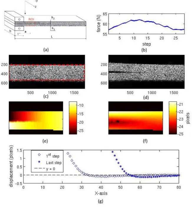
In this configuration, the sample is loaded in an opening mode as presented in Fig. 1a. The dimensions of the sample are b = 20 mm, h1 = 2.17 mm, h2 = 1.85 mm, L = 250 mm, and t = 20 mm.
The loading in the x-direction is performed along the perpendicular direction of the plies with a tension/compression servohydraulic testing machine. Before the experiment is started, the sample was pre-cracked over a length a. In practice, it is performed manually by the operator while carefully clamping the specimen ahead of the desired location. An alternative is to perform a first propagation step with the testing machine; this step is then not taken into account in the subsequent investigation. In the present case the first route was chosen. The sample is then loaded under a displacement controlled procedure in which the force is measured and an image is acquired at each of the 28 steps of interest (Fig. 1b). Figures 1c and 1d show the picture in the reference configuration and the last image in the deformed configuration of the ROI (Region of Interest, see Fig. 1a). The different images are used to measure the displacement field via Q4-DIC. In the present case, the edge size of each Q4 element is equal to 16 pixels (≈ 200 µm). The longitudinal (x-axis) and the transverse (y-axis) displacement fields between these two images are shown in Figs. 1e and 1f, where the pixel size is equal to 12 µm.
The presence of a crack is clearly visible in the image of the deformed configuration (Fig. 1d) and on the transverse displacement field (Fig. 1f). Figure 1g shows the mode I crack opening
5
displacement for the first and the last analyzed picture. It illustrates the change of crack opening and the resulting compression, in the right part, where the displacement jump is negative. In the present case, the crack opening displacement is evaluated as the difference of mean displacement of the two layers of the sample.
2.2. CLS configuration
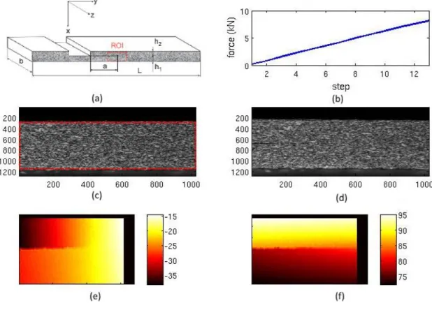
Figure 2a shows the loading for the CLS configuration. The dimensions of the sample are b = 10 mm, h1 = 1.61 mm, h2 = 1.57 mm, and L = 250 mm. It consists of a tensile test in a servohydraulic testing
machine where the plies are aligned along the loading direction. In this configuration, a pre-crack is manually created in the specimen by the operator while carefully clamping the two arms of the specimen. Thirteen loading steps are analyzed (Fig. 2b) and the corresponding images are acquired. Figures 2c and 2d show the picture in the reference configuration and in the deformed configuration at the end of the analysis. In this present case the edge size of each Q4 element is equal to 32 pixels (≈ 200 µm). The physical size of one pixel is now 3.5 µm since a higher magnification was selected (i.e., to enable for a more local analysis of the cohesive zone model). In this configuration, a mixed mode condition is induced by the experiment itself [12], which evolves during propagation. The presence of the crack is observed when analyzing the displacement fields. However, it is impossible to detect manually on the pictures since the mode I opening displacement is very small.
3.
Identification procedure of cohesive parameters
3.1. Mesh generation
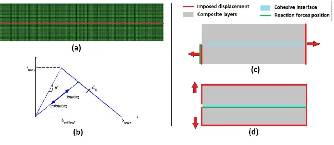
The numerical model is implemented in the commercial finite element code Abaqus [29]. A 2D Finite Element (FE) model is developed considering the plane stress assumption (Fig. 3a). Each part of the carbon-epoxy composite is meshed with CPS4 elements. The interface is modelled thanks to zero thickness 4-noded cohesive elements (COH2D4). The Dirichlet boundary conditions are based on the measured displacement field umeas from Q4-DIC analyses (Figs. 1 and 2). Therefore, the whole
6
experiment is not modeled but only the ROI monitored for DIC purposes [11, 12]. In Ref. [12], a minimum mesh refinement of two is advised. In the present case, a factor four on the refinement is selected to ensure an accurate description of the nonlinear stress shape behind the crack tip. It was checked that a finer mesh would lead to very similar results. In the numerical model, the prescribed displacements of these additional nodes are obtained with the Q4 interpolation functions of the measurement mesh. Since the Q4-DIC code CorreliSTC provides measured displacement fields using meshes made of Q4 elements, this interpolation is direct and does not add any additional error contrary to local DIC approaches.
3.2. Constitutive behavior
The behavior of the composite layers is assumed to be elastic. The elastic properties of each 0-degree laminate are E1 = 120GPa, E2 = E3 = 8.9GPa, G12 = 5.3GPa, ν13 = ν12 = 0.33, ν23 = 0.35 where 1 is
the longitudinal direction of the ply, 2 is the transverse one, and 3 the out-of-plane direction. These values were obtained from previous identification campaigns where several tensile tests with loading and unloading sequences were performed on [0°], [±45°], [±67.5°] coupons tested on an electrohydraulic testing machine, in the same manner as Ref. [32].
The cohesive zone model is characterized by a traction-separation law, which depends on the fracture energy and the strength of the interface (Fig. 3b). The area under the traction-displacement jump curves for a pure mode I or II is the respective fracture energy dependent on the critical crack opening displacement, final
i
i i c fin a l id
t
G
0 (1)7
The nominal traction, t, consists of two components in 2D problems, namely, tn and tt that represent
the normal and the shear tractions, respectively. The corresponding displacement jumps are δn and
δt. Denoting by h0 the original thickness of the cohesive element, the nominal strains are defined as
h
i i 0 (2)where i = n or t. The elastic behavior (Fig. 3b) of the interface is written as
t n tt nt nt nn t n K K K K t t
(3)where the off-diagonal terms in the stiffness matrix (i.e., Knt) are set to zero in order to express the
uncoupled behavior between normal and shear components.
In this work, a built-in CZM in Abaqus code is chosen even though the final goal is to use “bell-shape” models [4, 14, 15]. This is not detrimental to the present work whose purpose is the feasibility of the methodology rather than the details of the chosen CZM. For pure mode I or II loadings, after the interfacial normal or shear tractions reach their respective interlaminar tensile or shear strengths, the stiffnesses are gradually reduced to zero (Fig. 3b) via a damage parameter [14-16, 19]. As a first proposal and among the few equations proposed within the FE code, the coupling of the fracture energy under mixed mode condition is defined in terms of the Benzeggagh-Kenane criterion [33] so that the total fracture energy, C
G , is expressed as
T t C n C t C n CG
G
G
G
G
G
(
)
(4)8
where
G
T
G
n
G
tand is set to 1 (meaning that the 2D propagation space is a triangle, whichis valid as a first approximation).
3.3. Inverse identification method
To identify the cohesive parameters, which are gathered in vector θ, a cost function
(θ) is based on the comparison of the measured and simulated displacement fields and resultant forces
2 1 _ 2 _ _ _ _ _ _ _ _ 2 _ _ _ _ _ _ _ _ 2 _ _ _ _ _ _ _ _ 2 _ _ _ _ _ _ _ 2 ~ ~ 2 ~ ~ 2 ~ ~ 2 ~ ~ DCB step sensor F DCB DCB T DCB DCB total step sensor CLS step CLS dof DCB step DCB dof DCB step sensor DCB step DCB dof u DCB DCB T DCB DCB total step sensor CLS step CLS dof DCB step DCB dof DCB step DCB dof CLS step sensor F CLS CLS T CLS CLS total step sensor CLS step CLS dof DCB step DCB dof CLS step sensor CLS step CLS dof u CLS CLS T CLS CLS total step sensor CLS step CLS dof DCB step DCB dof CLS step CLS dof N N F F F F N N N N N N N N N N U U U U N N N N N N N N N N F F F F N N N N N N N N N N U U U U N N N N N N N N DCB DCB CLS CLS
θ θ θ θ θ θ θ θ θ (5)where Ndof is the number of kinematic degrees of freedom,
N
sensor the number of load sensors andstep
N the number of loading steps for each experiment.
U
~
and
F~ are the vectors gathering the measured displacements and forces, respectively,
U
and
F
, which depend on the parametersθ, the calculated displacement and force vectors,
u and
F the standard displacement and forceresolutions, respectively. In the present case, weighted residuals are considered that stem from a Bayesian foundation to account for the standard resolution levels associated with Q4-DIC and the load sensors. The underlying hypothesis is that noise is Gaussian and white. The quadratic form is the argument of the exponential in the Gaussian probability distribution. The additivity of the functionals is the counterpart of the statistical independence of the two measurements (i.e. load and
9
displacements), which implies that probabilities are multiplied. The chosen normalization by the noise amplitude in all functionals guarantees that no additional prefactors are to be considered. If only noise is present (i.e., no model error), the expectation of
(θ) is equal to 1 [34-36].The standard displacement resolution
u 0.04pixelin both cases (or 0.5 µm for the DCBexperiment, and 0.15 µm for the CLS experiment), whereas the standard load resolution is
N
1
DCBF
and
FCLS
50
N
. The identification of θ is performed through the minimization of thecost function through Broyden–Fletcher–Goldfarb–Shanno (BFGS) algorithm [37].
3.4. Boundary condition selection
It is worth noting that in all analyzed cases, experimental (i.e., measured) Dirichlet boundary conditions are applied to the numerical model. Consequently, any mode mixity induced by the stacking sequence (e.g., if not symmetric) or by any delamination plane not exactly located at mid-thickness (i.e., h1 h2) and/or loading conditions will be accounted for. These real conditions are often not taken into account in classical methods. In a previous work, it was shown that global mode mixities could be extracted by following such an approach [12].
A first identification route consists of prescribing the displacement on the whole boundary of the analyzed ROI in the CLS experiment as for the determination of global parameters [12]. Since displacements are prescribed, they will give rise to equilibrium gaps [38]. The equilibrium gap is separated into 8 contributions. Along the laminate (x-) direction the right and left reaction forces should be equal to the applied load (Fig. 3c-d). The right and left forces should be equal to 0 as well as the upper and lower ones. The identification leads to results with displacement residuals close to levels obtained for a global model [12] (i.e., a root mean square difference between measured and computed displacements ≈ 0.3 pixel). For the equilibrium constraint, the load residual is of the order of 200 N on each boundary except on the boundaries where forces are transmitted (right and left
10
boundaries along the laminate direction). On these boundaries, the cumulated residual is greater than 1,400 N. The same conclusion is drawn for the DCB test.
For the DCB experiment, it is possible to circumvent this issue by comparing the resultant of the cohesive load with the measured load (Fig. 3c). Conversely, for the CLS experiment, the upper and lower boundary conditions are stress-free in the simulations. Thus, the equilibrium gap is only built with the resultant load on the right side, which is equal to that of the lower left boundary (Fig. 3d).
4.
Sensitivity analyses
To determine the feasibility of the identification, a sensitivity (S) analysis is performed on the whole set of cohesive parameter θk [39], for all the spatial domain (x) and for all relevant time steps (t) of
the tests. This pre-analysis is carried out by means of the sensitivity matrix and allows for the best choice of identification strategy (e.g. two sets of parameters identified consecutively or only one set identified in one step). These parameters are the 6 cohesive properties and for the DCB test the crack initiation force. The latter is needed to account for the fact that the interface has been initially loaded at a level that is unknown. The sensitivity of the displacement field and resultant forces, collectively denoted by P, is written as
) , , ( ) , , ( ) , ( t t k k t k k
x P x P x S (6)and quantifies the effect of a variation θk of each parameter θk on the measured quantifies P. In the
following analyses, a parameters variation of 1% is prescribed. The higher the sensitivity the easier the identification of the corresponding parameter provided the levels of the sensitivity fields can be made greater than the measurement resolutions [34].
11
The following analysis is performed with the initial values of the sought parameters, namely, Knn = 39 GPa/mm, Ktt = 15 GPa/mm, σn = 15, MPa, σt = 37 MPa, GI = 350 J/m², and GII = 1500 J/m².
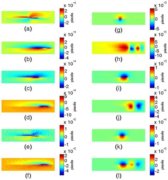
These parameters are representative of values used at Airbus Group Innovations for such class of materials. Moreover, a pre-loading at 60 N is chosen for the DCB test. This force corresponds to a preloading performed before the measurement to localize the crack tip. Figure 4 shows the displacement sensitivity maps of the last loading step of the DCB experiment for each parameter. As expected, very small influences of the tangential parameters (i.e., Ktt, σt, GII) are observed on the
displacements (< 10-5 pixel). When compared with the standard displacement resolutions they are significantly smaller, thereby proving that this experiment does not give any indication on the shear contribution of the CZM. On the contrary, the normal parameters lead to higher sensitivities, in particular the strength σn (10-4 pixel in the longitudinal direction, 10-3 pixel in the transverse
direction), but also the stiffness Knn and the toughness GI in the longitudinal direction (10-4 pixel).
However, these levels are still lower than the measurement resolution (greater than 10-2 pixel). The fact that all three normal parameters exhibit the same type of sensitivity is due to crack propagation that occurs for the last 16 steps of the experiment [12].
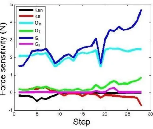
Without any additional information, there is no hope of identifying the cohesive parameters with the considered approach (i.e., cost function only driven by displacement). The same analysis is carried out for the load sensitivities in the loading direction for which measured data are available. Figure 5 shows that the sensitivity levels of the normal parameters are higher than the load resolution (of the order of 1N) in particular for the strength and toughness and to a lesser extent for the stiffness. This result explains why it is mandatory (at least for this configuration) to use a specific cost function that combines displacement and load measurements.
A similar analysis is performed for the CLS test. Figure 6 illustrates the displacement sensitivity maps of the last step of the CLS experiment, and Figure 7 the load sensitivity for all loading steps. Extremely low sensitivities are observed for both toughnesses. This result is to be expected
12
since it is believed that propagation was very limited for the last recorded picture [12] and the present FEMU process averages all steps. Conversely, the sensitivities to tangential and normal stiffnesses and strengths are more pronounced. This is due to the fact that the experiment was not in pure mode II loading [12]. There are strong correlations between normal and tangential parameters when displacements alone are analyzed. This is to be expected since no absolute stress (or load) scale is accounted for. As for the DCB test, the load sensitivities are very informative since their level is again higher than the load resolution for four out of 6 parameters (Figure 7). In both cases, the load information is crucial if cohesive parameters are sought.
In order to illustrate the global sensitivity to each parameter, the sensitivity matrix [M], which corresponds to the approximate Hessian of the nonlinear least squares formulation (5), is expressed as
jt ij i
M
S
ˆ
S
ˆ
(7)where
Sˆ
j is either the vector gathering one component of the nodal displacements over space and time, or all the load sensitivities over time for given parameter variations. The sensitivity matrices are shown for the DCB and CLS experiments in Figure 8. A high level in the sensitivity matrix represents a significant influence of the observed parameter, and a high level of off-diagonal terms suggests inter-dependencies between parameters as well.For the DCB test, the displacement along the vertical direction shows that only the parameters Knn and σn are sensitive and strongly correlated (i.e., nonzero off-diagonal terms). For the
horizontal direction, the parameters Knn, Ktt, σn and σt are the most sensitive. Moreover, the
parameters Knn and σn are strongly correlated in addition to Ktt with σt. Concerning the reaction
forces, only the normal parameters (i.e., Knn, σn, GI) are linked and very influent (i.e., significantly
13
For the CLS experiment, the parameter Ktt is the most sensitive in the horizontal direction. In
the vertical direction, Knn and Ktt are the most sensitive and not too (anti-)correlated. Concerning the
reaction forces, all the parameters (i.e., normal and tangential) are influential. This result confirms again the benefit to use such a combined cost function, i.e. mixing displacement and load measurements.
5.
Identification of cohesive parameters
This section presents the results of the parameter identification. Several protocols are considered based on the previous sensitivity analysis. First, using only the CLS experiment (i.e., a priori mode II dominant [6]) the tangential behavior is analyzed with a high stiffness and strength in the normal direction (i.e., only the part related to the CLS test is considered in the cost function (5) with three unknown parameters). Then, a similar analysis is performed for the normal parameters using the DCB experiment (i.e., only the part related to the DCB test is considered in the cost function (5) with 3 unknown parameters). Once a first set of the six parameters is obtained, they will be used separately to update them by following the same approach as before, considering a sequential identification protocol. Last, with the two previously determined levels of cohesive parameters, the complete set of cohesive parameters is simultaneously identified by analyzing both tests with the coupled cost function
introduced in Equation (5).5.1. First series of independent identifications
This first part aims to identify the tangential parameters using the CLS test. In order to identify them, the normal behavior is kept constant and chosen close to a purely elastic behavior (i.e., Knn = 500
MPa/mm, σn = 250 MPa, GI = 400 J/m²) with a high level for initiation. The results are presented in
Table 1 for different sets of bounds and initial values. Even though the three different sets of parameters are not identical, their level of variation remains small and that of the cost function is
14
very close. The values of each parameter with the lowest cost function is considered for the subsequent identification steps, namely, Ktt = 32 GPa/mm, σt = 17 MPa, and GII = 1200 J/m².
The identified toughness GII is consistent with the level found by a global elastic identification
when extrapolated to the failure load (1300 ± 50 J/m² [12]). Let us also note that the cost function has a level that is equal to about 7 times the standard resolutions associated with displacement and load measurements. This is an indication of a model error since if no model error had occurred, the cost function would be unitary. Conversely, the fact that its level does not depart too much from 1 is an indication that the model should not be disqualified at this stage.
Table 1: Tangential cohesive parameters identified when analyzing the CLS experiment for different bounds and initial values. The normal parameters are set to high values
Bounds Ktt (GPa/mm) 15 – 70 10 – 60 15 – 80 σt (MPa) 10 – 60 5 – 70 15 – 70 GII (J/m²) 700 - 1800 700 – 1800 700 - 1800 Initial values Ktt (GPa/mm) 35 20 30 σt (MPa) 18 23 32.5 GII (J/m²) 1100 1600 1200 Identified values Ktt (GPa/mm) 34 32 47 σt (MPa) 19 17 27 GII (J/m²) 1100 1200 890 Cost function (-) 7.55 7.53 7.57
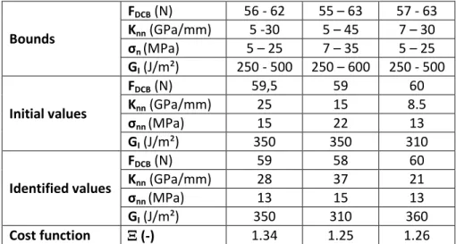
Second, the normal parameters are identified using the DCB test. As in the previous case, the tangential behavior is assumed constant and purely elastic (i.e., Ktt = 500 MPa/mm, σt = 250 MPa, and
GII = 1300 J/m²). The results gathered in Table 2 show that depending on the initial set of parameters
the converged solution is not identical. However, all lie within the chosen bounds. In the present case, the three solutions are not as close in terms of overall level of the cost function as for the CLS experiment. This is presumably due to the existence of secondary minima in the cost function since its level at convergence is very close for the three sets of parameters. The set of values
15
corresponding to the lowest cost function is chosen for subsequent analyses, namely, F = 58 N, Knn = 36 GPa/mm, σn = 15 MPa, and GI = 310 J/m².
The identified toughness GI has a level lower than that identified with an elastic analysis
(410 ± 50 J/m² [12]) yet with an identical order of magnitude. The level of the cost function is very close to the standard resolutions associated with displacement and load measurements. A very small model error is obtained in the present case, thereby validating it in the present analysis.
Table 2: Normal parameters identified when analyzing the DCB experiment for different bounds and initial values. The tangential parameters are set to high values
Bounds FDCB (N) 56 - 62 55 – 63 57 - 63 Knn (GPa/mm) 5 -30 5 – 45 7 – 30 σn (MPa) 5 – 25 7 – 35 5 – 25 GI (J/m²) 250 - 500 250 – 600 250 - 500 Initial values FDCB (N) 59,5 59 60 Knn (GPa/mm) 25 15 8.5 σnn (MPa) 15 22 13 GI (J/m²) 350 350 310 Identified values FDCB (N) 59 58 60 Knn (GPa/mm) 28 37 21 σnn (MPa) 13 15 13 GI (J/m²) 350 310 360 Cost function (-) 1.34 1.25 1.26
5.2. Second series of independent identifications
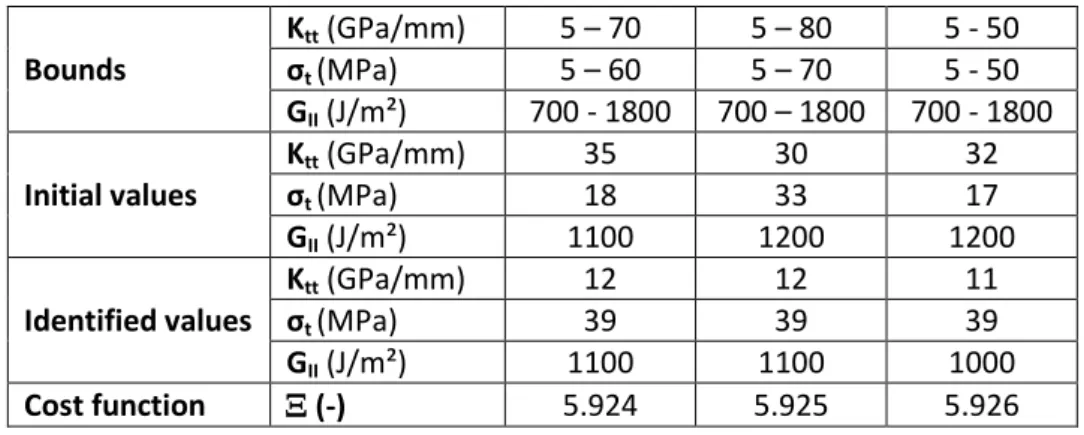
In this second loop, the tangential parameters are tuned by considering the values of the previously identified normal parameters, which still remain constant in the present minimization (F = 58 N, Knn = 36 GPa/mm, σn = 15 MPa, and GI = 310 J/m²). The results are presented in Table 3. As in the
previous cases, depending on the initial guess the converged solution is different. The identified tangential parameters are Ktt = 12 GPa/mm, σt = 39 MPa, GII = 1100 J/m².
16
The identified toughness GII is still close to the level found with a global elastic identification
(1300 ± 50 J/m² [12]). Interestingly, the level of the cost function has been reduced by 20% (i.e., from 7.5 to 5.9) with this step. This decrease is in part due to the change of the tangential parameters so that the minimization procedure is initialized with another set of parameters. This result confirms what was expected from the sensitivity analysis, namely, that normal and tangential parameters had the same level of influence for the displacements. In particular, the stiffnesses Knn
and Ktt were correlated as well the strengths σn and σt.
Table 3: Tangential parameters identified when analyzing the CLS experiment for different bounds and initial values. The normal parameters are set as the mean values of the previous identification
step Bounds Ktt (GPa/mm) 5 – 70 5 – 80 5 - 50 σt (MPa) 5 – 60 5 – 70 5 - 50 GII (J/m²) 700 - 1800 700 – 1800 700 - 1800 Initial values Ktt (GPa/mm) 35 30 32 σt (MPa) 18 33 17 GII (J/m²) 1100 1200 1200 Identified values Ktt (GPa/mm) 12 12 11 σt (MPa) 39 39 39 GII (J/m²) 1100 1100 1000 Cost function (-) 5.924 5.925 5.926
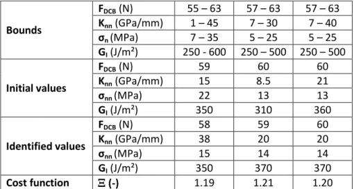
In order to identify the normal parameters, the tangential behavior is described with the previously identified parameters (i.e., Ktt = 12 GPa/mm, σt = 39 MPa, GII = 1100 J/m²). The results are
presented in Table 4. The identified tangential parameters are F = 58 N, Knn = 38 GPa/mm, σn = 15
MPa, and GI = 350 J/m². The identified parameters and the cost function levels are close to those of
Table 2 except for the stiffness Knn. Although the sensitivity is not strongly correlated between Knn
and the tangential parameters (i.e., Ktt, σt, GII), the Ktt parameter is slightly correlated with Knn and σn,
17
slightly reduced with this additional step. Being already close to 1, it was not expected to see significant changes when compared to those observed for the tangential parameters.
Table 4: Normal parameters identified when analyzing the DCB experiment for different bounds and initial values. The tangential parameters are set as the mean values of the previous identification
step Bounds FDCB (N) 55 – 63 57 – 63 57 – 63 Knn (GPa/mm) 1 – 45 7 – 30 7 – 40 σn (MPa) 7 – 35 5 – 25 5 – 25 GI (J/m²) 250 - 600 250 – 500 250 – 500 Initial values FDCB (N) 59 60 60 Knn (GPa/mm) 15 8.5 21 σnn (MPa) 22 13 13 GI (J/m²) 350 310 360 Identified values FDCB (N) 58 59 60 Knn (GPa/mm) 38 20 20 σnn (MPa) 15 14 14 GI (J/m²) 350 370 370 Cost function (-) 1.19 1.21 1.20 5.3. Combined identification
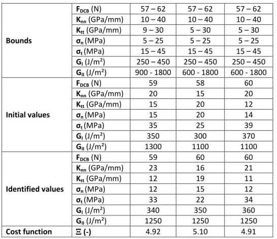
The last identification step consists of simultaneously identifying the normal and tangential cohesive parameters using both tests in a single analysis. The cost function is weighted accordingly. The results are gathered in Table 5. The level of the cost function is about five times the resolution limit, which validates the chosen model. The fact that this value lies between the two levels found by the two-step sequential identification procedure is expected thanks to the weighting introduced in Equation (5).
It is worth noting that the initial guesses analyzed in this part are all slightly different from the set found in Tables 3 and 4. The reason for this choice is to get some information about the sensitivity to the initial guess. The two lower residuals lead to parameters that are close (Table 5).
18
Table 5: Cohesive parameters identified when analyzing both experiments for different bounds and initial values Bounds FDCB (N) 57 – 62 57 – 62 57 – 62 Knn (GPa/mm) 10 – 40 10 – 40 10 – 40 Ktt (GPa/mm) 9 – 30 5 – 30 5 – 30 σn (MPa) 5 – 25 5 – 25 5 – 25 σt (MPa) 15 – 45 15 – 45 15 – 45 GI (J/m²) 250 – 450 250 – 450 250 – 450 GII (J/m²) 900 - 1800 600 - 1800 600 - 1800 Initial values FDCB (N) 59 58 60 Knn (GPa/mm) 20 15 20 Ktt (GPa/mm) 15 20 12 σn (MPa) 15 20 14 σt (MPa) 35 25 39 GI (J/m²) 350 300 370 GII (J/m²) 1300 1100 1100 Identified values FDCB (N) 59 60 60 Knn (GPa/mm) 23 16 21 Ktt (GPa/mm) 12 19 11 σn (MPa) 12 15 12 σt (MPa) 33 22 34 GI (J/m²) 340 350 360 GII (J/m²) 1250 1250 1250 Cost function (-) 4.92 5.10 4.91
The force used to initialize the simulation of the DCB test is very stable with a level of 59 ± 0.1 N. Among the six cohesive parameters, the level of confidence is very different. For the toughness GI its level (350 ± 15 J/m2) becomes closer to that found with a purely elastic identification
(410 ± 50 J/m² [12]). In the experiment, crack propagation is observed making its uncertainty very small. This phenomenon also explains the small fluctuation of the normal strength σn (13 ± 1.5 MPa).
Conversely, the identification of the normal stiffness is less stable even in the normal direction (Knn = 18 ± 3 GPa/mm).
The mean level GII (1250 ± 1 J/m²) is in very good agreement with a purely elastic identification when extrapolating the results for the failure load (1300 ± 50 J/m² [12]). The shear strength σt (28 ± 6 MPa) is more difficult to capture. The relative fluctuation of the tangential
19
stiffness (Ktt = 14 ± 4 GPa/mm) is of the same order of magnitude as that observed in the normal
direction.
In all analyzed cases, three different initial guesses were considered. The aim was to investigate the sensitivity of the CZM parameters to such initial values, and the level of the identification residual at the end of the optimization procedure. In general the level of the latter is very close, which indicates that overall calibration quality is similar. However, the values of some parameters are not necessarily close (i.e., Knn, Ktt and t), which proves that they cannot be calibrated
very precisely with the two considered experiments. Conversely, the evaluation of FDCB, GI, GII, and n
is more robust.
Interestingly, the two energy release rates are very well captured and consistent with analyses based upon linear elastic fracture mechanics [12]. The two stiffnesses are more difficult to evaluate quantitatively. They call for more accurate displacement measurements, but an order of magnitude is obtained, which is new for these types of tests. When the experiment allows stable propagation to occur, the strength of the CZM model can be estimated (i.e., n with the DCB
experiment). For the CLS test, the propagation steps were very limited and did not yield a robust estimate of the strength t.
6.
Conclusion
In this paper, two delamination tests are analyzed to determine the parameters modeling the cohesive behavior in mode I and II. A combined cost function is introduced to study both tests at the same time with a weighting based upon a Bayesian framework to account for all sources of uncertainty. In the present setting, the displacement correlations were neglected and only the standard displacement resolution was considered. It could be extended to include the various correlations thanks to the covariance matrix associated with the measured degrees of freedom [34, 35].
20
A sensitivity analysis is developed to illustrate the identification feasibility of the cohesive parameters. For the DCB test, the analysis shows a high sensitivity only for the normal behavior that illustrates a mode I loading. For the CLS test, which is a priori expected to be mode II-dominant for nominal boundary conditions, the sensitivity has the same level between the normal and tangential parameters, thereby indicating a mixed mode configuration, which is confirmed by previous analyses based upon full-field measurements [12]. One of the key conclusions of this analysis is that without load data the cohesive parameters are not identifiable with the two experimental configurations studied herein.
The identification procedure has been conducted by following a three-step approach. The first step consists of identifying separately and sequentially the normal and tangential cohesive parameters by analyzing one test at a time. The other parameters are set to levels representative of a pure elastic interfacial behavior. Once a first set of parameters is obtained, it can be used to initialize a second step that still analyses the two tests independently. The identification residuals allow the chosen model not to be disqualified. Last, the two tests are studied simultaneously and the seven parameters are varied at the same time. For this last step, the identification residuals amount to about 5 times the standard resolution of displacement and load data. This low level validates the cohesive model used herein. It is also shown that all the parameters can be identified and with an error indication that can be less than 1 % in the most favorable case up to 30 % in the most difficult instance. This result was obtained for different initial guesses of the sought parameters.
It is worth noting that having set the 7 parameters free directly, the identification would have been unstable. This is one of the reasons of the developed 3-step strategy thanks to the sensitivity analysis. The latter proves that the initial guess is very important. This calls for simplified and fast techniques to get initial estimates faster than by performing finite element simulations, which are very demanding when dealing with cohesive zone models. Since the mode I and II toughnesses identified with the present procedure are in good agreement when compared to linear elastic
21
fracture mechanics analyses [12], such type of approach is beneficial and leads to a more robust identification route. Systematic sensitivity analyses with quantitative estimations of uncertainties and errors are useful whatever the mode mixity of tests or configurations.
The present framework may also be used to identify initiation and propagation parameters under more complex configurations (e.g., interfaces between [±] plies) since it is very generic (i.e., it does not rely on closed-form solutions whose applicability is restricted to very simple cases). It has been shown that it is possible not only to extract global propagation parameters (e.g., GI and GII) but
also initiation values. Future analyses will also have to be extended to cases of rapid propagation to study delamination under dynamic loading conditions. One critical issue is related to the way the finite element simulations are driven with measured displacement fields that are corrupted by measurement uncertainties. Spatiotemporal DIC analyses may be used to tackle such difficult problems [40].
Acknowledgement
The support of this research by “Agence Nationale de la Recherche” is gratefully acknowledged (VULCOMP Phase 2 project, Grant No. ANR-12-RMNP-0018)
22
References
[1] Irving P, Soutis C. Polymer Composites in te Aerospace Industry. Amsterdam (the Netherlands): Elsevier; 2014.
[2] Baker A, Dutton S, Kelly D. Composite Materials for Aircraft Structures. AIAA Education Series. Reston, VA (USA): AIAA; 2004.
[3] Davies P, Blackman BRK, Brunner AJ. Standard Test Methods for Delamination Resistance of Composite Materials: Current Status. Appl Compos Mat. 1998 5(6):345-64.
[4] Allix O, Blanchard L. Mesomodeling of delamination: towards industrial applications. Comp Sci Tech. 2006;66(6):731-44.
[5] ASTM. D5528 - 01e3 Standard Test Method for Mode I Interlaminar Fracture Toughness of Unidirectional Fiber-Reinforced Polymer Matrix Composites. West Conshohocken, PA (USA): ASTM; 2007.
[6] ASTM. D5868 - 01 Standard Test Method for Lap Shear Adhesion for Fiber Reinforced Plastic (FRP) Bonding. West Conshohocken, PA (USA): ASTM; 2008.
[7] IGC. 4.26.381. Instruction Générale de Contrôle pour détermination du G1c. Aérospatiale standard1991.
[8] AITM. 1.0005. Determination of interlaminar fracture toughness energy. Airbus Industrie Test Method1994.
[9] Ireman T, Thesken JC, Greenhalgh E, Sharp R, Gädke M, Maison S, et al. Damage propagation in composite structural elements-coupon experiments and analyses. Comp Struct. 1996;36:209-20.
[10] Abanto-Bueno J, Lambros J. Investigation of crack growth in functionally graded materials using digital image correlation. Eng Fract Mech. 2002;69:1695-711.
[11] Fedele R, Raka B, Hild F, Roux S. Identification of adhesive properties in GLARE assemblies by Digital Image Correlation. J Mech Phys Solids. 2009;57:1003-16.
[12] Mathieu F, Aimedieu P, Guimard J-M, Hild F. Identification of interlaminar fracture properties of a composite laminate using local full-field kinematic measurements and finite element simulations. Comp Part A. 2013;49:203-13.
[13] Cui W, Wisnom MR. A combined stress-based and fracture-mechanics-based model for predicting delamination in composites. Compos. 1993;24, :467-74.
[14] Allix O, Ladevèze P, Corigliano A. Damage analysis of interlaminar fracture specimens. Compos Struct. 1995;31:66-74.
[15] Allix O, Corigliano A. Modeling and simulation of crack propagation in mixed-modes interlaminar fracture specimens. Int J Fract. 1996;77:111-40.
[16] Chaboche JL, Girard R, Levasseur P. On the interface debonding models. Int J Damage Mech. 1997;6(3):220-57.
[17] Reddy Jr. ED, Mello FJ, Guess TR. Modeling the initiation and growth of delaminations in composite structures. J Compos Mat. 1997;31:812-31.
[18] Barenblatt GI. The Mathematical Theory of Equilibrium of Crack in Brittle Fracture. Adv Appl Mech. 1962;7:55-129.
[19] Hillerborg A, Modeer M, Petersson PE. Analysis of crack formation and crack growth in concrete by means of fracture mechanics and finite elements. Cement Conc Res. 1976;6:773-82.
[20] Dugdale DS. Yielding of Steel Sheets Containing Slits. J Mech Phys Solids. 1960;8:100-4.
[21] Döll W, Könczöl L. Micromechancis of fracture: optical interferometry of crack tip craze zone. Adv Polym Sci. 1990;91-92:138-214.
[22] Abanto-Bueno J, Lambros J. Experimental Determination of Cohesive Failure Properties of a Photodegradable Copolymer. Exp Mech. 2005;45(2):144-52.
[23] Xu XP, Needleman A. Void nucleation by inclusions debonding in a crystal matrix. Modelling Simul Mater Sci Eng. 1993;1:111-32.
23
[24] Besnard G, Hild F, Roux S. ``Finite-element'' displacement fields analysis from digital images: Application to Portevin-Le Châtelier bands. Exp Mech. 2006;46:789-803.
[25] Hong S, Chew HB, Kim KS. Cohesive-zone laws for void growth - I. Experimental field projection of crack-tip crazing in glassy polymers. J Mech Phys Solids. 2009;57:1357-73.
[26] Ferreira MDC, Venturini WS, Hild F. On the analysis of notched concrete beams: From measurement with Digital Image Correlation to identification with Boundary Element Method of a cohesive model. Eng Fract Mech. 2011;78:71-84.
[27] Shen B, Paulino GH. Direct Extraction of Cohesive Fracture Properties from Digital Image Correlation: A Hybrid Inverse Technique. Exp Mech. 2011;51:143-63.
[28] Fuchs PF, Major Z. Experimental determination of Cohesive Zone Models for Epoxy Composites. Exp Mech. 2011;51:779-86.
[29] Réthoré J, Estevez R. Identification of a cohesive zone model from digital images at the micron-scale. J Mech Phys Solids. 2013;61(6):1407-20.
[30] Simulia. Abaqus Analysis User's Manual (version 6.7). 2010. [31] http://www.holo3.com/correli-stc®-afr17.html. 2012.
[32] Ladevèze P, Le Dantec E. Damage modelling of the elementary ply for laminated composites. Comp Sci Tech. 1992;43(3):257-67.
[33] Benzeggagh ML, Kenane M. Measurement of Mixed-Mode Delamination Fracture Toughness of Unidirectional Glass/Epoxy Composites With Mixed-Mode Bending Apparatus. Comp Sci Tech. 1996;56:439-49.
[34] Gras R, Leclerc H, Hild F, Roux S, Schneider J. Identification of a set of macroscopic elastic parameters in a 3D woven composite: Uncertainty analysis and regularization. Int J Solids Struct. 2015;55:2-16.
[35] Mathieu F, Leclerc H, Hild F, Roux S. Estimation of Elastoplastic Parameters via Weighted FEMU and Integrated-DIC. Exp Mech. 2015;55(1):105-19.
[36] Bertin M, Hild F, Roux S, Mathieu F, Leclerc H, Aimedieu P. Integrated Digital Image Correlation applied to elasto-plastic identification in a biaxial experiment. J Strain Analysis. 2016;51( 2):118-31.
[37] Matlab. Matlab, the Language of Technical Computing, version R2015a: the MathWorks, inc. (http://www.mathworks.com); 2015.
[38] Claire D, Hild F, Roux S. Identification of damage fields using kinematic measurements. C R Mécanique. 2002;330:729-34.
[39] Tarantola A. Inverse Problems Theory. Methods for Data Fitting and Model Parameter Estimation. Southampton (UK): Elsevier Applied Science; 1987.
[40] Besnard G, Leclerc H, Roux S, Hild F. Analysis of Image Series through Digital Image Correlation. J Strain Analysis. 2012;47(4):214-28.
24
Figures
Figure 1: (a) DCB sample with the position of the Region Of Interest (ROI) used to measure displacement fields. (b) Load history. Pictures of (c) initial and (d) last loading steps (the coordinates
are expressed in pixels). Measured (e) vertical and (f) horizontal displacement fields (expressed in pixels) for the last loading step. (g) Displacement jump (expressed in pixels) profile for the first and
25
Figure 2: (a) CLS sample with the position of the Region Of Interest (ROI) used to measure displacement fields. (b) Load history. Pictures of (c) initial and (d) last loading steps (the coordinates
are expressed in pixels). Measured (e) vertical and (f) horizontal displacement fields (expressed in pixels) for the last loading step
26
Figure 3: (a) Finite element mesh in which the cohesive nodes are marked in red. (b) Illustration of the cohesive law. (c) Boundary conditions for the CLS experiment. (d) Boundary conditions or the DCB experiment
27
Figure 4: Displacement (expressed in pixel) sensitivity maps of the DCB test for the last loading step in horizontal (left), and vertical (right) directions for a 1% variation of each cohesive parameter.
28
Figure 5: Reaction force sensitivity as a function of the loading step in the DCB experiment for a 1% variation of each cohesive parameter
29
Figure 6: Displacement (expressed in pixel) sensitivity maps in the CLS test for the last loading step in horizontal (left), and vertical (right) directions for a 1% variation of each cohesive parameter.
30
Figure 7: Reaction force sensitivity as a function of the loading step in the CLS experiment for a 1% variation of each cohesive parameter
31
Figure 8: Sensitivity matrix for the DCB experiment (left) for the displacement field in the horizontal (a), in the vertical direction (c), and for the cohesive reaction force (e). Sensitivity matrix for the CLS experiment (right) for the displacement field in the horizontal (b), in the vertical direction (d), and for