Prediction of VOC concentration profiles in a newly constructed house using small chamber data and an IAQ simulation program

Publisher’s version / Version de l'éditeur:

Journal of Indoor Air - Special Issue - Papers from Indoor Air 2002, pp. 1-33,

2002-07-01

READ THESE TERMS AND CONDITIONS CAREFULLY BEFORE USING THIS WEBSITE. https://nrc-publications.canada.ca/eng/copyright

Vous avez des questions? Nous pouvons vous aider. Pour communiquer directement avec un auteur, consultez la

première page de la revue dans laquelle son article a été publié afin de trouver ses coordonnées. Si vous n’arrivez pas à les repérer, communiquez avec nous à PublicationsArchive-ArchivesPublications@nrc-cnrc.gc.ca.

Questions? Contact the NRC Publications Archive team at

PublicationsArchive-ArchivesPublications@nrc-cnrc.gc.ca. If you wish to email the authors directly, please see the first page of the publication for their contact information.

Archives des publications du CNRC

This publication could be one of several versions: author’s original, accepted manuscript or the publisher’s version. / La version de cette publication peut être l’une des suivantes : la version prépublication de l’auteur, la version acceptée du manuscrit ou la version de l’éditeur.

Access and use of this website and the material on it are subject to the Terms and Conditions set forth at

Prediction of VOC concentration profiles in a newly constructed house

using small chamber data and an IAQ simulation program

Magee, R. J.; Lusztyk, E.; Won, D. Y.; Shaw, C. Y.

https://publications-cnrc.canada.ca/fra/droits

L’accès à ce site Web et l’utilisation de son contenu sont assujettis aux conditions présentées dans le site LISEZ CES CONDITIONS ATTENTIVEMENT AVANT D’UTILISER CE SITE WEB.

NRC Publications Record / Notice d'Archives des publications de CNRC:

https://nrc-publications.canada.ca/eng/view/object/?id=a980b670-3b49-4981-a826-21ae60344e4c https://publications-cnrc.canada.ca/fra/voir/objet/?id=a980b670-3b49-4981-a826-21ae60344e4c

Prediction of VOC concentration profiles in a newly constructed

house using small chamber data and an IAQ simulation program

Magee, R.J.; Lusztyk, E.; Won, D.Y.; Shaw, C.Y.

NRCC-46731

A version of this document is published in / Une version de ce document se trouve dans :

Indoor Air 2002, Monterey, California, June 30-July 5, 2002, pp. 1-33

PREDICTION OF VOC CONCENTRATION PROFILES IN A NEWLY

CONSTRUCTED HOUSE USING SMALL CHAMBER DATA AND AN IAQ

SIMULATION PROGRAM.

RJ Magee

, E Lusztyk

, DY Won

and CY Shaw

1

Indoor Environment Program, Institute for Research in Construction, National Research Council of

Canada, Ottawa, Ontario, K1A 0R6, Canada.

FAX: (613) 954-3733

Abstract

The ability of the Material Emission Database and Indoor Air Quality simulation program (“MEDB-IAQ”) to use small chamber test results to model volatile organic compound (VOC) profiles in a newly constructed 2-storey single family home was evaluated. Selected building materials used in the construction of the CCHT (Canadian Centre for Housing Technology) “Reference” house were collected and subjected to chamber testing. VOC emission rates were modeled from the results and entered into MEDB-IAQ. A simulation of the house construction and subsequent operation for an additional nine months was then run with the software package. Air exchange rate data from the house was also used as model input. Predicted VOC results were then compared with air samples taken from the house and analyzed by GC/MS. Prediction accuracy

depended on source complexity, source identification and emitting area, and on sink effects. Trends in relative contributions of individual materials could be readily identified.

Index Terms

VOC emissions; building materials; indoor air quality; modeling; simulation; chamber testing

Introduction

Volatile organic compounds (VOCs) in commercial and residential environments have typically been the focus of indoor air quality investigations (Hodgson and Wooley, ’91; Brown et al., ’94; Gammage and Bervin, ’96; Jones, ’99; Spengler et al., ’01; Brown ’02; Wolkoff and Nielsen, ’01). While the sources of VOCs indoors can be attributed to building furnishings, indoor activities, outdoor air, or the building occupants themselves, materials used in initial construction and/or building renovation are frequently implicated (Mølhave ’78 and ’82; Hodgson and Girman ’83; Girman et al., ’84; Tichenor and Mason ‘88; Tucker ’90; Levin ’96; Levin and Hodgson ’96; Wolkoff ’96; ECA-IAQ ‘97; Maroni and Lundgren ’98; Yu and Crump ’98; Zhu et al., ‘98). Identification of building materials as VOC sources led to the need for standard test methods for determining emission rates from these products (Tichenor ‘87; ASTM ’97; Wolkoff ’99). Emissions testing can only be effective if appropriate sampling and analytical technologies are in place to capture, identify and quantify VOCs of interest.

While our understanding of the toxicological impact of complex mixtures of VOCs common to indoor air remains limited, recognition that individual VOC species may have markedly different impact has generally led to the abandonment of the concept of Total VOC (TVOC) as an indicator of air quality. This has in turn led to growing efforts to develop lists of “target” VOCs (Wolkoff et al., ’97; Levin, ’98; Mølhave ’98; Maroni and Lundgren, ’98; Seppanen ’98; Hoddinott and Lee, ’02). Secondary by-products of VOCs, generated through reactions with, for example, ozone may also be responsible for IAQ problems, thus the interest in the study of “indoor chemistry” (Weschler et al., ’92; Weschler and Shields, ’97; Knudsen et al. ’00; Weschler ’00; Wolkoff et al.,’00). This also has impact on the discernment of “target” VOCs (the parent VOC, though relatively harmless, may become a valid “target” if it’s secondary products are harmful). Realistic guidelines for acceptable indoor air or for regulation of emissions from building materials will develop in conjunction with these efforts to distinguish those VOCs with significant impact on IAQ (Nielsen et al., ’97; Levin and

Alevantis, ‘03).

Once reliable testing protocols for determining the emissions of appropriate “target” VOCs from building materials have been established, comparison of individual products becomes possible, leading to the

development of product certification and ranking schemes. Several early attempts at this have been initiated, even though acceptance of a list of “target” compounds is yet to be achieved (Canilli et al., ’93; Johnston et al., ’96; Kukkinen et al., ’02; Oppl ’99; Witterseh ’02). Variability inherent in many building materials (by virtue of material inhomogeneity and/or manufacturing process changes) should be factored into any such product-product comparisons (Oppl and Winkels, ’02; Magee et al, ’03).

The need also arises for efficient and accessible storage of emissions test data. Several database systems have been or are being developed for this purpose (Bluyssen et al., ’00; Claussen et al., ’96; Jensen and Wolkoff, ’96; Howard-Reed et al., ’03; Park and Ikeda, 03).

Modeling of emissions from building materials is the next logical step in determining their impact on indoor environments. Whether empirical in nature (derived from chamber test results) or based on mass transfer fundamentals (and validated by chamber testing), the development of emission models has been an area of

keen interest (Guo and Tichenor ‘92; Won, Shaw et al., ’01; Yang et al., ‘01a and ‘01b). “Sink” effect (both the reversible and irreversible sorption of VOCs) must be considered as it has a significant impact on the accuracy of models that attempt to predict indoor concentrations of emitted VOCs (Tichenor ’96; Won, Sander, et al. ’01; Won, Corsi and Rynes, ’01).

This paper deals with validation trials conducted with a combination emissions database and simulation tool for estimating indoor VOC concentrations due to building materials. The database/simulation package, called MEDB-IAQ (for Materials Emission DataBase and IAQ simulation program) was developed at the Institute for Research in Construction (IRC) of the National Research Council of Canada as one of the deliverables of the Consortium for Material Emissions and IAQ Modeling (CMEIAQ) Project. The MEDB-IAQ package allows users to: 1) select building materials from a database of carefully controlled chamber tests of VOC emissions, 2) specify building ventilation rates and schedules, and, 3) use a single zone model to predict resultant VOC concentrations.

An opportunity to evaluate MEDB-IAQ’s capabilities arose with the construction of identical two-story research houses at the Canadian Centre for Housing Technology (CCHT) at the IRC campus in Ottawa, Ontario, Canada. Built in partnership with Natural Resources Canada and Canada Mortgage and Housing Corporation, IRC operates the houses as a platform for evaluating new housing technologies. The

woodframe units were built to R-2000 specifications, including high efficiency forced gas heating coupled with heat recovery ventilation (HRV). The “Reference” house, which was built to serve as a stable baseline for changes introduced into the “Research” house, was the subject of this investigation. Floor area of the 4-bedroom house was 204.5 m2. The interior volume was 794.3 m3. Complete access to and control over the construction of the reference house enabled direct collection of building material specimens for chamber testing, as well as an unrestricted ability to conduct IAQ-related evaluations of the house for the nine-month period following the completion of the house.

The ability of MEDB-IAQ to store emissions test data for materials collected from the house, and then to use this data to predict VOC levels within the house is the focus of this paper. This work is an extension of

previously reported efforts with MEDB-IAQ to use small chamber data to predict full-scale chamber tests of selected building material assemblies (Biesenthal et al., ’02).

Methods

The methods employed in this study can be sub-divided into the four major tasks described below.

Documentation of house construction / specimen collection

On-site lab personnel inspected the construction site daily throughout the entire construction phase and maintained a detailed log of all construction activities at the house. A photographic record taken immediately on the site was supplemented by an automated camera mounted on an adjacent building overlooking the site which recorded digital images at regular intervals. Specimens of building materials were collected directly from the site as they arrived. These were identified, coded and sealed in Tedlar sampling bags (or in glass vials or original packaging for “wet” construction materials) for storage in the lab prior to emissions testing. The exposed interior surface areas of all building materials in the house were carefully measured and recorded.

House characterization / IAQ testing

House operation. An automated occupancy simulation system was designed to mimic typical behavior of a

family within the house. Remotely monitored and controlled, this system operated appliances in the house (stove, dishwasher, clothes dryer and washing machine), adjusted lighting conditions, ran kitchen and bathroom faucets/toilets/showers and exhaust systems, adjusted heating and cooling setpoints, and simulated occupant heat loads through activation of balanced lamps in different locations of the house.

Air change rate monitoring. Commencing with the “completion” of the house (i.e. construction finished,

house ready for “occupancy”), the air change rate in the house was monitored on a daily basis via the tracer decay and constant concentration methods (automated injection and sampling of sulfur hexafluoride using a Brûel and Kjær Model 1302/1303 multigas monitor/sampler/doser system. Samples were also periodically analyzed via gas chromatography/electron capture detection to confirm the B&K data.

Environmental monitoring. An automated data acquisition system continuously monitored an extensive

network of temperature and relative humidity sensors within and outside the house. For approximately nine months following completion of the house, a second data acquisition system was also installed for continuous monitoring of carbon dioxide and ozone levels. Periodic sampling was also conducted to monitor levels of carbon monoxide, nitrogen dioxide, sulfur dioxide, and suspended particulates.

VOC sampling/analysis. Levels of VOCs within the house were determined through air sampling on

Carbotrap 300 sorbent tubes followed by thermal desorption (Perkin-Elmer ATD400) and GC/MS analysis (Hewlett Packard Models 5890 / 5989). VOC sampling was conducted daily for the first week after

completion of the house, twice weekly for the next week, once a week for the 3rd and 4th weeks, once every two weeks for weeks 5 through 8, and then approximately every other week until the end of the nine month monitoring period.

“Total Volatile Organic Compounds” (TVOC) in this study is a semi-quantitative measure defined as the sum of individual VOC concentrations (both identified and noidentified) in the range from pentane to n-hexadecane as determined by the GC/MS response factor for Toluene. TVOC was used only as an estimator of the magnitude of VOC emissions from a given product and as an indicator of the MEDB-IAQ simulation’s success at identifying VOC sources.

Individual “Target” Volatile Organic Compounds were selected for quantitative monitoring in the house air samples based on the following considerations:

• The “Target” VOC was found to be relatively abundant in the house air samples, • The “Target” VOC was emitted from materials with significant emitting surface areas, • The “Target” VOCs should cover a wide range of volatility (i.e. test capability of MEDB-IAQ

simulation for diverse chemical species), and

• priority was given to VOCs that had been identified in existing material labeling programs and/or health agency lists.

The concentrations of the 13 “Target” VOCs were determined using their respective GC/MS response factors (i.e. individual chemical standards were obtained for each target compound and the GC/MS system’s

response determined for a dilution series of each). The concentrations of the target VOCs were measured for the entire nine-month monitoring period.

Aldehydes sampling/analysis. In addition to the GC/MS analysis of VOCs found in the house air, periodic

sampling for low molecular weight aldehydes (formaldehyde, acetaldehyde, acrolein, propionaldehyde,

butyraldehyde and benzaldehyde) was conducted using Waters Sep-Pak XpoSure samplers. These

were then extracted with acetonitrile and analyzed by high performance liquid chromatography (HPLC) using a Varian Model 9012 Solvent Delivery System and Model 9050 UV-Vis Detector. The column used was a Supelcosil LC-18. Calibration of the system was conducted using dilutions prepared from Supelco 4-7649 Carb-Carbonyl-DNPH standard mixtures.

Building material emissions tests / Calculation of emission coefficients:

VOC emissions tests of the building material specimens were conducted in 50L electropolished stainless steel chambers according to guidelines specified in ASTM D5116 (ASTM 1997). Chamber conditions were 23oC, 50% relative humidity and an air change rate of 1 hr-1. Stainless steel specimen holders were used to limit the exposed surface area of the test specimens in a manner that approximated the emitting surfaces of the materials in the house. Details of the testing protocols can be found in Bodalal et al. (2000). The following individual building materials collected from the CCHT Reference house were tested in the 50L chambers: plywood, oriented strand board (OSB), engineered I-beam floor joists (OSB/spruce); drywall, latex primer, latex paint, varnish, woodstain, caulking, carpet, underpad, and adhesive for ceramic wall tiles. In addition, a specimen of the wallboard was primed and painted prior to mounting in the specimen holder, and then tested as a material “assembly”. Although not reported here, tests were also conducted of the “low-VOC” content latex paint and water-based varnish and woodstain that were used in the Research house as alternative to traditional products. Portions of the kitchen cabinets were also tested separately in IRC’s full-scale chamber.

Details of the procedures used to determine emission coefficients from the chamber concentration vs. time data have been previously reported (Magee et al., ’99; Zhu, et al., ’99). For “dry” materials a power law model was employed to fit the emission characteristics between 24 and 120 hours. The emission characteristics of the wet building materials (paint/primer, stains, caulking) were determined using the segmented VB-power law model (Guo Z, Tichenor BA. 1992). .

Simulation of VOC emissions in the Reference House

The MEDB-IAQ package has been described previously (Zhang, Shaw, et al., ’99; Zhang, Zhu, et al., ’99; Won et al., ’03). For this investigation, the details of the specimens collected from the CCHT Reference house, their chamber test conditions and the calculated model coefficients from the emissions data were added to the MEDB-IAQ database. MEDB-IAQ’s simulation tool was then used to predict VOC

concentrations in the CCHT Reference House by mimicking the entry of the selected building materials into the house, at air change rate conditions designed to approximate the actual conditions observed over the simulation period. Building materials were selected for simulation based on their source strengths (from the chamber tests) and their exposed surfaces areas in the house. The selected materials, their surface areas and the air change conditions for the simulation are summarized in Table 1. Note that in several cases the material installations were split over several days to more accurately reflect construction practices. The simulated emitting surface areas ranged from 0.1 m2 (caulking) to ~ 566 m2 for the painted wallboard. Chamber data for the material assembly of paint/primer/wallboard was used in the simulation, rather than individual values for these three materials.

Table 1: Summary of key simulation inputs.

Activity in House Time,

days

Surface

Area, m2

Air change

rate, hr-1

add I-Beam floor joist -118 28.7 50

add I-Beam floor joist -117 28.7 50

add OSB Subfloor -118 34.8 50

add OSB Subfloor -117 34.8 50

add Particleboard (stairs) -97 1.5 50

House envelop completed -52 0.12

Caulk basement windows -51 0.1 0.12

Prime/Paint gypsum Wallboard -26 283.2 0.12 Prime/Paint gypsum Wallboard -25 283.2 0.12

Stain stair railings -25 5.0 0.12

Plywood subfloor in kitchen -22 5.6 0.12

install Carpeting -11 63.5 0.12

install Carpeting -8 63.5 0.12

Varnish stair railings -4 5.0 0.12

House construction complete 0 0.12

HRV System operating 27 0.23

add OSB shelves in basement 41 5.0 0.23

As indicated in Table 1, simulation time zero was defined as the point of “completion” of the house (construction fully complete, all appliances and systems fully installed and operational, house in condition equivalent to turn-over to new owners in real world). Construction of the house commenced 134 days earlier (foundation poured), while the first simulated building material was the I-beam floor joists and OSB subfloor that was installed at day –118. Closure of the house envelope occurred at day –52 (all walls, roof, doors and windows installed). Prior to this time, an arbitrary value of 50 air changes per hour was used to simulate the “open” condition of the house. An average air change rate of 0.12 hr-1 was used based on tracer gas tests conducted prior to the point at which the house’s HRV unit was balanced (27 days after “completion”). The simulated air change rate was then set at 0.23 hr-1, which represented an average value of the tracer decay results from the remainder of the test period. VOC concentrations were calculated at 1h intervals for the 10,000 hour simulation period (approx. 14 months) commencing with the house foundation pour.

Results and discussion

IAQ evaluation of the Reference House

The IAQ investigation of the CCHT Reference House provided the following observations:

• TVOC concentrations were highest during the first week after closure, then decreased with time, becoming relatively stable about 40 days after the house closure at approximately one quarter of the maximum observed level. This pattern was also noted for those individual VOCs whose initial concentrations, at the closure of the Reference house, exceeded 0.25 mg/m3 (decane, undecane,

toluene, and α-pinene).

• Levels of compounds whose initial concentrations were between 0.01 and 0.20 mg/m3 (nonane,

dodecane, 1,2,4-trimethylbenzene, limonene, hexanal, and methyl ethyl ketone or “MEK”) generally

showed a slight decrease after about 40 days.

• The concentrations of compounds whose initial levels were below 0.01 mg/m3 (1,4-dichlorobenzene,

styrene, and 4-PC), typically did not change significantly during the entire monitoring period (within 0.005

mg/m3). Among these three compounds, the concentration of styrene changed most during the first 10 days (from approximately 0.005 mg/m3 to about 0.002 mg/m3). The slight increase observed in the concentration of 1,4-dichlorobenzene after about 150 days (from 0.0002 to 0.0007 mg/m3) was within measurement uncertainties.

• Air samples taken simultaneously at multiple locations in the house indicated relatively uniform concentrations for VOCs with vapor pressures ranging from 0.27 to 86.95 mm Hg, indicating good air mixing in the house.

• The concentrations of all identified individual VOCs were found to be below their respective “lowest concentration of interest” (LCI) suggested by the European Commission Joint Research Centre-Environment Institute (ECA-IAQ 1997). Most were at least an order of magnitude lower than their LCI value. Toluene and α-pinene levels were closest to their LCI level.

• The concentration of formaldehyde observed in the Reference house exceeded Health Canada’s Target Level of 60 µg/m3 (Health Canada 1995) for most of the monitoring period. It also exceeded the Action Level (120 µg/m3) during the first week after the closure and on two additional occasions during the first 30 days.

• The CO2 concentration in the unoccupied Reference house was below 500 ppm. The average O3

concentration was 2.2 ppb with a standard deviation of 1.1 ppb during the monitoring period. The concentration of sulfur dioxide (SO2) remained below the detection limit (0.1 ppm) for the entire

the gas fireplace was tested and once when soldering of copper tubing occurred in the house. Nitrogen dioxide (NO2) were below the detection limit (0.5 ppm) except on one occasion.

• The suspended particulate concentration in the CCHT Reference houses was similar to that in a normal office environment, and was only about 22-35% of the outdoor particulate concentration measured. • The heat recovery ventilator provided fairly stable outdoor air changes to the house (0.23 ± 0.046

ACH during the monitoring period).

As in indication of the complexity of the VOC “fingerprint” of the house, figure 1 shows the chromatogram of an air sample taken in the house 93 days after “completion”. Approximately 80 different VOCs were identifiable in the sample.

5.00 10.00 15.00 20.00 25.00 30.00 35.00 40.00 45.00 0 50000 100000 150000 200000 250000 300000 350000 400000 450000 500000 550000 600000 650000 700000 Time--> Abundance TIC: 99042305.D 35 34 33 31 30 29 27 22 18 17 13 10 2 2 Methylethyl ketone 10 Hexanal 12 Octane 13 Toluene 17 Trimethyl benzene 18 α−Pinene 22 Limonene 27 Nonane 29 Decane 30 Undecane 31 Dodecane 33 Cyclohexane 34 Styrene 35 4-PC CCHT House at Day 93

Figure 1: Chromatogram of air sample taken on day 93 in Reference house.

Building material emissions tests

As examples, chromatograms of air samples taken from the test chambers after 24 hours are given for the caulking specimen and for the paint/primer/drywall assembly, respectively, in Figures 2 and 3. Full

descriptions of the VOCs emitted by the material specimens collected from the CCHT houses have been reported separately (Bodalal et al., ’00). GC/MS analysis of the air samples from the chamber tests of the 12 building materials identified almost 200 individual VOCs. Four to six VOCs per material were selected for detailed analysis / modeling / input into MEDB-IAQ.

5.00 10.00 15.00 20.00 25.00 30.00 35.00 40.00 45.00 0 10000 20000 30000 40000 50000 60000 70000 80000 90000 100000 110000 120000 130000 140000 150000 160000 170000 180000 Time--> Abundance TIC: 98120121.D 8 13 12 27 30 29 31 17

Caulking

Figure 2: Chromatogram of air sample from caulking test after 24 hours.

5.00 10.00 15.00 20.00 25.00 30.00 35.00 40.00 45.00 0 5000 10000 15000 20000 25000 30000 35000 Time--> Abundance TIC: 00020206.D 4 3 2 1 Paint-Primer-Drywall Assembly 1 2 3 4 1 1-Butanol 2 n-Butyl Ether 3 Texanol 1 4 Texanol 2

Figure 3: Chromatogram of air sample from paint/primer/wallboard assembly test after 24 hours.

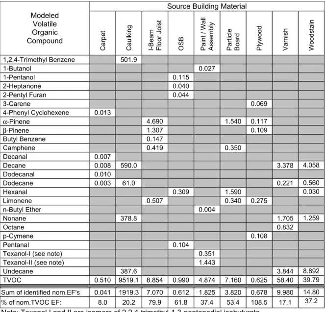
Table 2 provides a summary of the nominal emission factors (at 24 hours) for TVOC and individual VOCs calculated from the chamber data for the tested CCHT building materials. Note that the list is not an

exhaustive one for any of the tested materials. The intent was only to model sufficient VOC concentrations to permit evaluation of MEDB-IAQ’s capability to predict emissions in the house. In the case of the carpet specimen for example, the five modeled VOCs accounted for only 8% of the total VOC emission of the

material. In contrast, due to the relatively simple profile of emitted VOCs typical of plywood, in this case the five VOCs selected represented essentially the full emissions of this material (the sum of the five individual emission factors actually exceeding the TVOC factor, indicating the error inherent in the TVOC analysis). The relative VOC source strengths of the tested materials is clearly indicated by the magnitude of the

emission factors shown. Hence the significant impact of the caulking on the VOC profile of the CCHT house, despite its extremely small emitting area (Table 1).

Table 2: Summary of Nominal Emission Factors (mg/m2h at 24 hours) from CCHT materials.

Source Building Material Modeled Volatile Organic Compound Carp et Caulk in g

I-Beam Floor Joist OSB Paint / Wall Assembly Particle Board Plywo

od Varnis h W oodstai n 1,2,4-Trimethyl Benzene 501.9 1-Butanol 0.027 1-Pentanol 0.115 2-Heptanone 0.040 2-Pentyl Furan 0.044 3-Carene 0.069 4-Phenyl Cyclohexene 0.013 α-Pinene 4.690 1.540 0.117 β-Pinene 1.307 0.109 Butyl Benzene 0.147 Camphene 0.419 0.350 Decanal 0.007 Decane 0.008 590.0 3.378 4.058 Dodecanal 0.010 Dodecane 0.003 61.0 0.221 0.560 Hexanal 0.309 1.590 0.030 Limonene 0.507 0.340 0.275 n-Butyl Ether 0.004 Nonane 378.8 1.705 1.259 Octane 0.832 p-Cymene 0.108 Pentanal 0.104

Texanol-I (see note) 0.351 Texanol-II (see note) 1.443

Undecane 387.6 3.844 8.892 TVOC 0.510 9519.1 8.854 0.990 4.874 7.160 0.625 58.40 39.79 Sum of identified nom.EF's 0.041 1919.3 7.070 0.612 1.825 3.820 0.678 9.980 14.80 % of nom.TVOC EF: 8.0 20.2 79.9 61.8 37.4 53.4 108.5 17.1 37.2

MEDB-IAQ simulation results

The material descriptions and modeled VOC emission coefficients were entered into MEDB-IAQ’s database function, while the volume and air change conditions representing the CCHT reference house were input into the simulation design component of the package and the building material areas and addition times were programmed according to the values in Table 1. Running the simulation yielded the following results.

0.00001 0.001 0.1 10 1000 0.0001 0.01 1 100 10000 -120 -90 -60 -30 0 30 60 90 120 150 180 210 240 270 300 Carpet Caulking Eng'd I-Beam OSB SubFloor OSB Shelves Paint+Wall Particleboard Plywood Woodstain Varnish TVOC N=50 N=0.12 N=0.23

OPEN TIGHT NORMAL

Elapsed Time from House Completion, days

P

redi

c

ted TVOC Concentrati

o

n, m

g

/m

3

Figure 4. TVOC levels – Predicted contribution of individual building materials.

Figure 4 shows the predicted contributions of the modeled materials to the TVOC levels in the house over the course of the ~ 400 day simulation period. House “completion” is indicated by time “0” on the x-axis. The three modeled air change zones are indicated on the figure as “open”, “tight” and “normal”, resulting in step change shifts in the predicted VOC levels. Spikes in the VOC profiles reflect entry points of the different

building materials. Several observations can be made from this figure: the simulation predicts that the impact of the woodstain, while significant over the short-term, will be minimal over the long term due to its rapid decay in emission rate. In contrast, products such as the engineered I-beam floor joists and the OSB sub flooring, will become dominant over time by virtue of their slowly decaying emission profiles. As mentioned previously, the relatively tiny amount of caulking in the house (small strip used to seal one of the basement windows) has a dramatic impact on the VOC level in the house.

Predicted profiles for individual VOCs in the house are shown in Figure 5. The rapid removal of highly volatile n-Butyl Ether and 1-Butanol following the application of the woodstain is clearly indicated. This is again in contrast to the slow decay in the levels of α-Pinene, Pentanal and 4-PC.

0.000001 0.00001 0.0001 0.001 0.01 0.1 1 10 100 1000 10000 -120 -90 -60 -30 0 30 60 90 120 150 180 210 240 270 300 1-Butanol 4-PC α-Pinene Decane n-Butyl Ether Pentanal Texanol I Texanol II TVOC N=50 N=0.12 N=0.23

OPEN TIGHT NORMAL

Elapsed Time from House Completion, days

Predicted VO

C Co

ncen

tr

a

ti

o

n

, mg

/m

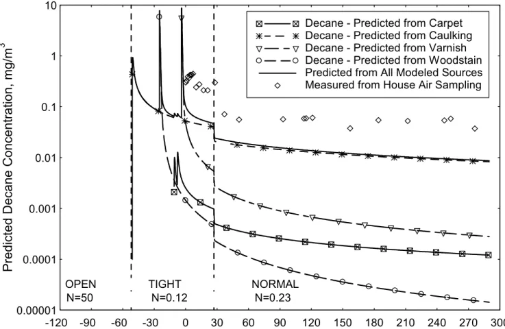
Figure 6 demonstrates the ability of the MEDB-IAQ simulation to predict the contribution of individual building materials to the indoor levels of a particular VOC, in this case decane. While decane emission was predicted from four materials, caulking is clearly the dominant source. Also shown in this figure are the actual

measured values of decane in the house. The simulation significantly under-predicts the indoor concentration of this particular compound. Several explanations exist for this discrepancy. Perhaps all decane sources in the house were not modeled (likely since decane is emitted by a large number of materials). Sink effect also appears to be acting here. On days 0 through 10, while the modeled results predict rapid decay in decane levels (from spike caused by application of varnish to stairwell trim), the air samples from the house analysed by GC/MS indicate a rising decane concentration. This is consistent with initial sink of the emitted decane and subsequent re-emission into the indoor air.

0.00001 0.0001 0.001 0.01 0.1 1 10 -120 -90 -60 -30 0 30 60 90 120 150 180 210 240 270 300

Decane - Predicted from Carpet Decane - Predicted from Caulking Decane - Predicted from Varnish Decane - Predicted from Woodstain Predicted from All Modeled Sources Measured from House Air Sampling

N=50 N=0.12 N=0.23 OPEN TIGHT NORMAL

Elapsed Time from House Completion, days

Predic

ted D

e

c

ane C

onc

ent

rat

ion,

mg/

m

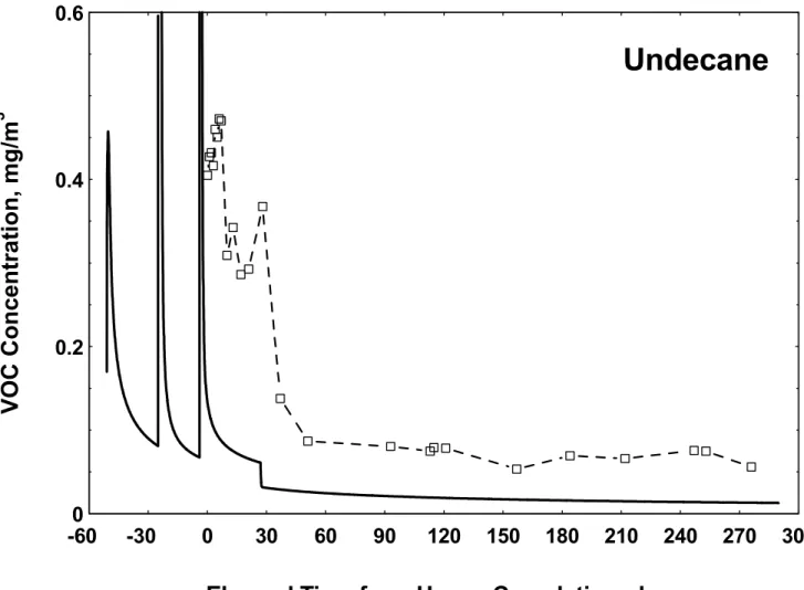
The remaining figures compare modeled and measured indoor levels for individual VOCs. Good agreement was found between predicted and observed levels of Trimethyl Benzene (Figure 7). This is likely due to the fact that this VOC was relatively unique to the caulking material used selectively in the house, thus the source was well defined as was the emitting surface area. The alkanes (nonane, decane, undecane and dodecane; Figures 8-11) all tended to be under-predicted, again probably reflecting incomplete source identification and/or sink effects stemming from high spike concentrations of these compounds. Levels of α -pinene were also under-predicted (Figure 12), conceivably due to source underestimation (large surface areas of wood framing hidden in walls, but likely in contact with the indoor air through various leakage paths. Figure 13 reveals an over-estimation of the indoor concentration of 4-PC, perhaps reflecting the testing of a non-representative specimen of the carpeting from the house. Hexanal and limonene showed erratic behavior in the GC/MS samples. They were also detected at relatively low concentration and are known to be difficult to quantify by the GC/MS conditions used in this study. Still the simulated concentrations were reasonably close to the measured values.

The final figure (Figure 16), shows predicted and measured TVOC levels. Not surprisingly, there is significant disagreement here. Un-modelled sources, and analytical difficulties in accurately measuring TVOC are likely error causes. Additionally, it is evident that while the simulation case used a constant air change rate of 0.23 hr-1 for the “normal” period, the air change test results clearly show that the amount of outdoor air entering the house dropped after approximately day 170 of the test (coinciding with the shift to air conditioning mode and the beginning of summer). Rising temperature and humidity levels observed in the house at this time would also contribute to the observed rise in TVOC levels in defiance of the predicted decay.

Conclusions

The MEDB-IAQ package provides a useful tool for storing emissions data from building material tests. The accuracy of its predictions of indoor VOC levels is dependent on a number of factors including:

• good chamber testing data from representative materials,

• accurate identification of all sources for any given VOC, coupled with • reasonable estimation of the effective emitting areas of the sources,

• accurate measurement of air change conditions for the simulated environment, and

• knowledge of the impact of environmental conditions such as temperature and humidity on VOC emissions.

Despite the obvious impact of these factors on the simulation, the predicted concentrations for most individual VOCs showed reasonable agreement with the measured concentrations in the CCHT reference house. The package’s potential to provide useful information to researchers and designers seems to be indicated. It provides a convenient platform for evaluating the relative impact of different building materials on the indoor environment or for assessing their concentration profiles under various ventilation conditions. A number of improvements currently in process (including expanded capabilities to deal with variable air change rate conditions) should further improve the usefulness of this tool. Ongoing improvements to models for VOC emissions will also be incorporated as they develop. The database of emissions test results will be continuously expanded, as will the modeling of an ever-evolving list of “target” compounds.

Acknowledgements

Jianshun Zhang was project manager for the research leading to the initial development of the MEDB-IAQ model and the establishment of the chamber testing methods that form the basis of the VOC emissions database. Dan Sander has provided essential input in the ongoing development of the MEDB-IAQ package. Marcel Brouzes and Awad Bodalal conducted the chamber emission tests of the building material specimens. The partners in the CCHT Project are gratefully acknowledged (www.ccht-cctr.gc.ca).

REFERENCES

ASTM (1997) ASTM Standard D5116 “Standard Guide for Small-Scale Environmental Chamber

Determinations of Organic Emissions From Indoor Materials/Products”. American Society for Testing and Materials.

Biesenthal, T., Magee, R.J., Bodalal, A., Lusztyk, E., Brouzes, M.A., Nong, G., Shaw, C.Y. (2002) “Upscaling of material emissions: comparison of small and full-scale chamber results and evaluation of an IAQ simulation model”. Proceedings of Indoor Air 2002, 9th International Conference on Indoor Air Quality and Climate, Monterey, California, Vol.3, pp.310-315.

Bluyssen, P.M., Fernandes, E. de Oliveira, Molina, J.L. (2000) “Database for sources of pollution for healthy and comfortable indoor environment (SOPHIE): Status 2000” Proc. Healthy Buildings (Aug.2000), Vol.2, 385-390.

Bodalal, A., Lusztyk, E., Shaw, C.Y., Magee, R.J., Brouzes, M.A. (2000) “Field Validation of an IAQ Model for Predicting the Impact of Material Emissions on the Indoor Air Quality in a Newly Constructed House. Task II - Results of Emission Testing” National Research Council of Canada, Report B-3307.2

Brown, S.K. (2002), “Volatile Organic Pollutants in New and Established Buildings in Melbourne, Australia”,

Indoor Air, 12, 55-63.

Brown, S.K., Sim, M.R., Abramson, M.J., Gray, C.N. (1994) “Concentrations of volatile organic compounds in indoor air – A review”. Indoor Air, 4, 123-134.

Canilli, C. ,Johnston, P. ,Koontz, M.D. ,Girman, JR. ; Kennedy, P.W. (1993) “Ranking consumer/commercial products and materials based on their potential contribution to indoor air pollution”, Proc. Indoor Air ’93,

Vol.2, 425-430.

Clausen, G., de Oliveira Fernandes, E., Fanger, .PO. (1996) “European Data Base on indoor air pollution sources in buildings”, Proc. Indoor Air ’96,Vol.2, 639-644.

ECA-IAQ (1997) “Evaluation of VOC Emissions from Building Products: Solid flooring materials”. European Collaborative Action-Indoor Air Quality & Its Impact on Man: Environment and Quality of Life. Report 18. EUR 17334 EN.

Gammage, R.B., Berven, B.A.,(editors), (1996) ”Indoor air and human health”, Boca Raton : CRC Press, Girman, J.R., Hodgson, A.T. and Newton, A.S. (1984) "Volatile organic emissions from adhesives with indoor

applications". In: Berglund, B., Lindvall, T. and Sundell, J. (eds.) Proceeding of Indoor Air '84, Stockholm, Swedish Council for Building Research, Vol. 4, pp. 271-276.

Guo Z., Tichenor, B.A. (1992) “Fundamental mass transfer models applied to evaluating the emissions of vapor-phase organics from interior architectural coatings”. EPA/AWMA Symposium, Durham, NC. Hoddinott, K.B., Lee, A.P. (2002) ”The use of risk assessment methodlogies for an indoor air quality

investigation”, Chemosphere, 41, 77-84.

Hodgson, A.T., Girman, J.R. (1983) ”Emission of volatile organic compounds from architectural materials with indoor applications”.,Berkeley,California: Lawrence Berkeley Laboratory. [PICA ps85160558 (GBPSA)] Hodgson, A.T. and Wooley, J.D., (1991) “Assessment of Indoor Concentrations, Indoor Sources and Source

Emissions of Selected Volatile Organic Compounds”. California Air Resources Board, Sacramento, CA: Final Report, Contract No. A933-063.

Howard-Reed, C., Polidoro, B., Dols, W.S. (2003) “Development of a series of IAQ model input databases: Contaminant source emission rates”, Air and Waste Management Association Conference: IAQ Problems and Engineering Solutions, Durham, NC, July 20-23, 2003.

Jensen, B., Wolkoff, P. (1996) ”VOCBASE - Odor and muccous membrane irritation thresholds and other physico-chemical properties. Version 2.1”, National Institute of Occupational Health, Copenhagen, May 1996,

Johnston, Pauline K., Cinalli-Christina, A.,Girman, J.R., Kennedy, P.W. (1996) “Priority ranking and characterization of indoor air sources”,ASTM-Special-Technical-Publication. n 1287, Characterizing sources of indoor air pollution and related sink effects,392-400.

Knudsen, H.K., Nielsen, P.A., Clausen, P.A., Wilkins, C.K. and Wolkoff, P. (2000) “Sensory evaluation of the impact of ozone on emissions from building materials”, In: Proceedings Healthy Buildings 2000,

Seppanen, O.,Sateri,J. (Eds.) 217 222

Kukkonen, E., Saarela, K., Neuvonen, P. (2002) “Experiences from the emission classification of building materials in Finland”, Proceedings: Indoor Air 2002, 9th International Conference On IAQ and Climate, Monterey, Calif, June 30 - July 5, 2002, Vol.3, 588-592.

Levin, H. (1996) ”Estimating building material contributions to indoor air pollution” Indoor Air ’96, 7th

International Conference On IAQ and Climate, Volume 3, July 21-26, Nagoya, Japan, 723-728.

Levin, H. (1998) ”Toxicology-based air quality guidelines”, Indoor Air, Suppl.5, 5-7.

Levin, H., Alevantis, L. (2003) “California indoor air quality specifications for open office systems furniture and building materials” Air and Waste Management Association Conference: IAQ Problems and Engineering Solutions, Durham, NC, July 20-23, 2003.

Levin, H., Hodgson, A.T. (1996) ”Screening and selecting building materials and products based on their emissions of volatile organic compounds (VOCs)”,ASTM-Special-Technical-Publication. n 1287, Characterizing sources of indoor air pollution and related sink effects, 376-391.

Magee, R.J., Bodalal, A., Biesenthal, T.A., Lusztyk, E., Brouzes, M., and Shaw, C.Y. (2002) “Prediction of VOC concentration profiles in a newly constructed house using small chamber data and an IAQ simulation program”, Proceedings of Indoor Air 2002, 9th International Conference on Indoor Air Quality and Climate, Monterey, California, Vol.3, pp.298-303.

Magee, R.J., Zhu, J.P., Zhang, J.S., Shaw, C.Y. (1999) “Small Chamber Test Method for Measuring Volatile Organic Compound Emissions from "Dry" Building Materials” : Consortium for Material Emissions and IAQ Modeling (CMEIAQ) Final Report 1.2, 43 pp, A-3563.F1.2

Magee, R.J., Won, D., Shaw, C.Y., Lusztyk, E., Yang, W. (2003) “VOC Emissions from building materials - the impact of specimen variability - a case study. Air and Waste Management Association Conference: IAQ Problems and Engineering Solutions, Durham, NC, July 20-23, 2003.

Maroni, M., Lundgren, B. (1998),”Assessment of the Health and Comfort Effects of Chemical Emissions from Building Materials: the State of the Art in the European Union”, Indoor Air, Suppl.4, 26-31.

Mølhave, L. (1978) “Indoor air pollution due to building materials”. Proceedings of 1st International Climate Symposium. Copenhagen, Danish Building Research Institute, pp.89-110.

Mølhave, L. (1982) “Indoor air pollution due to organic gases and vapours of solvents in building materials”,

Environment International, 8, 117-127.

Mølhave, L. (1998),”Principles for Evaluation of Health and Comfort Hazards Caused by Indoor Air Pollution”,

Indoor Air, Suppl. 4, 17-25.

Nielsen, G.D.,Hansen, L.F.,Wolkoff, P. (1997),”Chemical and biological evaluation of building material emissions. II. Approaches for setting indoor air quality standards or guidelines for chemicals”, Indoor Air, 7, 17-32.

Oppl, R, Winkels, K. (2002) “Uncertainty of VOC and SVOC measurement - How reliable are results of chamber emission testing?”, Proceedings: Indoor Air 2002, 9th Int'l Conf. On IAQ and Climate, Monterey, Calif, June 30 - July 5, 2002,Vol.2,902-906.

Oppl, R. (1999),”The EMICODE labelling system for flooring installation products”., Proceedings: Indoor Air

'99, 8th Int'l Conf. On IAQ and Climate, Edinburgh, Scotland, Aug.8-13, 1999, Vol.1, 543-548.

Park, J.S.,Ikeda, K. (2003),”Database system, AFoDAS/AVDAS, on indoor air organic compounds in Japan”,

Indoor Air, 13, Suppl.6,35-41.

Reardon, J.T., Brouzes, M.A., Shaw, C.Y. (2003) “Field Validation of an IAQ Model for Predicting the Impact of Material Emissions on the Indoor Air Quality in a Newly Constructed House. Task 3 – Air Leakage”, National Research Council of Canada, Report B-3307.1

Seppanen, O.,(editor) (1998),”Indoor Air and Health - Causitive Agents, Health Hazards and Risk” Assessment, Indoor Air, Suppl.4.

Shaw, C.Y., Sander, D. M., Magee, R. J., Lusztyk, E., Reardon, J. T., Bodalal, A., Nong, G.; Biesenthal, T. A., Won, D. Y. (2001) “Material emissions and indoor air quality modelling project - an overview”, IAQVEC 2001, International Conference on IAQ & Energy Conservation (Changsha, China, Oct, 2001)

Spengler, J.D., Samet, J.M., McCarthy, J.F., (editors), (2001),”Indoor Air Quality Handbook”, McGraw Hill, Tichenor, B.A. (1987) "Organic emissions via small chamber testing". In: Seifert, B., Esdom, H., Fischer, M.,

Ruden, H. and Wegner, J. (eds.) Proceedings of Indoor Air '87, Berlin (West), Institute of Water, Soil and Air Hygiene, Vol. 1, pp.8-15.

Tichenor, B.A. (editor) (1996) “Characterizing sources of indoor air pollution and related sinks”, ASTM STP 1287.

Tichenor, B.A., Mason, M.A. (1988) “Organic Emissions from consumer products and building materials to the indoor environment”, Journal of the Air Pollution Control Association, 38, 264-268.

Tucker, W. G. (1990) "Building with low-emitting materials and products: where do we stand?" In: Walkinshaw, D.S. (ed.) Proceedings of Indoor Air '90, Ottawa, Canada Mortgage and Housing Corporation, Vol. 3, pp. 251-256.

Weschler, C.J. (2000) “Ozone in indoor environments:concentrations and chemistry”, Indoor Air , 10, 269-288.

Weschler, C.J., Hodgson, A.T.,Wooley, J.D. (1992), ”Indoor Chemistry: Ozone, volatile organic compounds and carpets”, Env.Sci.Technol., 26, 2371-2377.

Weschler, C.J.,Shields, H.C. (1997),”Potential reactions amoung indoor pollutants”., Atm.Environ., 31, 3487-3495.

Witterseh, T. (2002),”Status of the Indoor Climate Labelling scheme in Denmark”, Proceedings: Indoor Air

2002, 9th Int'l Conf. On IAQ and Climate, Monterey, Calif, June 30 - July 5, 2002,Vol.3, 612-614.

Wolkoff, P. (1996),”Characterization of emissions from building products: long-term chemical evaluation”,

Indoor Air,6,1,579.

Wolkoff, P. (1999) “How to measure and evaluate volatile organic compound emissions from building products. A perspective.” The Science of the Total Environment. Vol. 227, 197-213.

Wolkoff, P., Nielsen, G.D. (2001),”Organic compounds in indoor air - Their relevance for perceived indoor air quality?”, Atmospheric Environment, 35, 4407-4417.

Wolkoff, P.,Clausen, P.A.,Jensen, B.,Nielsen, G.D.; Wilkins, C.K. (1997),”Are we measuring the relevant indoor pollutants?”, Indoor Air, 7, 92-106.

Wolkoff, P., Clausen, P.A., Wilkins, C.K., Nielsen, G.D. (2000) “Formation of strong airway irritants in terpene/ozone mixtures”, Indoor Air, 10, 82-91.

Won, D.Y., Magee, R.J., Lusztyk, E., Nong, G., Zhu, J.P., Zhang, J.S., Reardon, J.T. and Shaw, C.Y. (2003) “A comprehensive VOC emission database for commonly-used building materials“, Healthy Buildings 2003, Singapore.

Won, D.Y., Sander, D.M., Shaw, C.Y., Corsi, R.L. (2001) “Validation of the surface sink model for sorptive interactions between VOCs and indoor materials”. Atmospheric Environment, 35, 4479-4488.

Won, D.Y., Corsi, R.L., Rynes, M. (2001) “Sorptive interactions between VOCs and indoor materials”, Indoor

Air, 11 (4), 246-256.

Won, D.Y., Shaw, C.Y., Biesenthal, T. Lusztyk, E., Magee, R. J. (2001) “Application of chemical mass balance modeling to indoor VOCs”, Proceedings of Indoor Air 2002, 9th International Conference on Indoor Air Quality and Climate, Monterey, California, Vol.__, pp.268-273.

Yang, X., Chen, Q., Zeng, J., et al. (2001) “A mass transfer model for simulating volatile organic compound emissions from 'wet' coating materials applied to absorptive substrates”. International Journal of Heat

and Mass Transfer, 44(9), 1803-1815.

Yang, X., Chen, Q., Zhang, J.S., et al. (2001) “Numerical simulation of VOC emissions from dry materials”.

Building and Environment, 36, 1099-1107.

Yu, C., Crump, D. (1998) “A review of the emission of VOCs from polymeric materials used in buildings”.

Building and Environment, 33 (6), 357-374.

Zhang, J.S., Magee, R.J., Lusztyk, E., Zhu, J.P., Reardon, J.T., Brouzes, M.A., Shaw, C.Y. (2000) “Field Validation of an IAQ Model for Predicting the Impact of Material Emissions on the Indoor Air Quality in a Newly Constructed House. Task 1 - Results of Field Measurements”, National Research Council of Canada, Report B-3307.1

Zhang, J.S., Shaw, C.Y., Sander, D., Zhu, J.P., Huang, Y. (1999) “MEDB-IAQ: A Material Emission Database and Single-Zone IAQ Simulation Program – A Tool for Building Designers, Engineers and Managers”. National Research Council Canada.

Zhang, J.S., Zhu, J.P., Magee, R.J., et al. (1999) “A Database of VOC emissions from building materials”.

First NSF International Conference on Indoor Air Health (Denver, Colorado, 5/3/99), 87-96.

Zhu, J.P., Magee, R.J., Zhang, J.S., Shaw, C.Y., (1999) “A Small Chamber Test Method for Measuring Volatile Organic Compound Emissions from "Wet" Building Materials” Consortium for Material Emissions and IAQ Modeling (CMEIAQ) Final Report 1.3, 31 pp,A-3563.F1.3

Zhu, J.P., Zhang, J.S., Lusztyk, E., Magee, R.J. (1998) “Measurements of VOC emissions from three building materials using small environmental chamber under defined standard test conditions”. Air & Waste Management Association 91st Annual Meeting & Exhibition (San Diego), pp 1-16.

0

0.05

0.10

0.15

0.20

-60

-30

0

30

60

90

120

150

180

210

240

270

300

Trimethyl Benzene

Elapsed Time from House Completion, days

VOC Concentration, mg/m

3

0

0.05

0.10

0.15

0.20

-60

-30

0

30

60

90

120

150

180

210

240

270

300

Nonane

Elapsed Time from House Completion, days

VOC Concentration, mg/m

3

0

0.2

0.4

0.6

0.8

1.0

-60

-30

0

30

60

90

120

150

180

210

240

270

300

Decane

Elapsed Time from House Completion, days

VO

C Concentr

a

tion, mg/m

3

0

0.2

0.4

0.6

-60

-30

0

30

60

90

120

150

180

210

240

270

300

Undecane

Elapsed Time from House Completion, days

VO

C Concentr

a

tion, mg/m

3

0

0.1

0.2

0.3

0.4

0.5

-60

-30

0

30

60

90

120

150

180

210

240

270

300

Dodecane

Elapsed Time from House Completion, days

VO

C Concentr

a

tion, mg/m

3

0

0.2

0.4

0.6

0.8

1.0

-60

-30

0

30

60

90

120

150

180

210

240

270

300

α

-Pinene

Elapsed Time from House Completion, days

VO

C Concentr

a

tion, mg/m

3

0

0.005

0.010

0.015

0.020

-60

-30

0

30

60

90

120

150

180

210

240

270

300

4-PC

Elapsed Time from House Completion, days

VO

C

Concentr

ation, mg/m

3

0

0.02

0.04

0.06

0.08

0.10

-60

-30

0

30

60

90

120

150

180

210

240

270

300

Hexanal

Elapsed Time from House Completion, days

VOC Concentration, mg/m

3

0

0.05

0.10

0.15

-60

-30

0

30

60

90

120

150

180

210

240

270

300

Limonene

Elapsed Time from House Completion, days

VOC Concentration, mg/m

3

0.1

1

10

100

-60

-30

0

30

60

90

120

150

180

210

240

270

300

0.1

1

10

100

Measured TVOC

Modelled TVOC

Measured Air Change Rate

Modelled Air Change Rate

TVOC

Elapsed Time from House Completion, days

TVO

C

Concentration, mg/m

3

Air Change Rate, hr

-1

List of Figures:

Figure 1: Chromatogram of air sample taken on day 93 in Reference house. Figure 2: Chromatogram of air sample from caulking test after 24 hours.

Figure 3: Chromatogram of air sample from paint/primer/wallboard assembly test after 24 hours. Figure 4. TVOC levels – Predicted contribution of individual building materials.

Figure 5. Predicted levels of individual VOCs in the house. Figure 6. Predicted vs. measured levels of decane in the house. Figure 7. Predicted vs. measured levels of trimethyl benzene. Figure 8. Predicted vs. measured levels of nonane.

Figure 9. Predicted vs. measured levels of decane. Figure 10. Predicted vs. measured levels of undecane. Figure 11. Predicted vs. measured levels of dodecane. Figure 12. Predicted vs. measured levels of α-pinene. Figure 13. Predicted vs. measured levels of 4-PC. Figure 14. Predicted vs. measured levels of hexanal. Figure 15. Predicted vs. measured levels of limonene. Figure 16. Predicted vs. measured levels of TVOC.