Application of Real Options to Evaluate the Development Process of New Aircraft Models

(1)

American Institute of Aeronautics and Astronautics 1

Application of Real Options to Evaluate the Development

Process of New Aircraft Models

Bruno Miller*_{and John-Paul Clarke}†

International Center for Air Transportation Department of Aeronautics and Astronautics

Massachusetts Institute of Technology Cambridge, Massachusetts

Investment decisions in the development and production of new aircraft models is difficult because of the technical and market uncertainties associated with such a complex process. The accompanying risks can be mitigated through a flexible approach that incorporates several decision points at different stages of the process. Therefore, as the project evolves, management will be able to diagnose its progress, compare it to previous expectations, and decide to continue or not. In this paper, we present a methodology to evaluate flexible business strategies that is based on real options analysis (ROA) and Monte Carlo simulation. This methodology takes into account the flexibility that managers have to affect the success of any given project and, therefore, it provides a better estimate of project value. Numerical results are given for a representative process based on actual aircraft manufacturer’s data.

I. Introduction

Investment decisions in the development and production of new aircraft models is difficult because of the risks associated with such a complex process. Air transportation is a cyclical industry characterized by periods of high growth followed by periods of deep traffic reductions.1, 2_{For example, in the United States, demand for aviation}

services, measured in terms of revenue-passenger miles (RPMs‡_{), had a robust growth from 1982 to 1987 (see}

Figure 1). It then experienced a decline which was exacerbated by the Gulf War in 1991. After this, the industry entered a period of strong recovery throughout the 1990s. This bonanza started to decline in early 2001 and plummeted after the attacks of September 11th_{of the same year. Since then, the path to recovery has been slow but}

steady. -6% -1% 4% 9% 14% 1980 1982 1984 1986 1988 1990 1992 1994 1996 1998 2000 2002 Gr o w th r ate (%) RPM GDP

Figure 1: The demand growth rate for air transportation in the United States domestic market is cyclical. Airline demand is measured in terms of revenue-passenger miles (RPMs). Source: The authors with data from ATA (2004) and BEA (2004).

*_{Research Assistant, International Center for Air Transportation, Massachusetts Institute of Technology,}

Cambridge, MA 02139. Student member AIAA.

†_{Assistant Professor, International Center for Air Transportation, Massachusetts Institute of Technology,}

Cambridge, MA 02139. Associate Fellow AIAA.

(2)

Planning in the face of the volatility of traffic demand becomes a major challenge for all stakeholders, in particular airlines, aircraft manufacturers and airports. The long lead times associated with production of new aircraft, with construction of new assembly lines or with delivery of new passenger buildings may result in these investments not arriving at the appropriate time: a premature investment may result in unused capacity that sits idle without generating any returns whereas a tardy investment may miss the potential market completely.

In order to address these risks and make the project more attractive to investors, a flexible approach that incorporates several decision points at different stages of the process is recommended. Therefore, as the project evolves, management will be able to diagnose its progress, compare it to previous expectations, and decide to continue or not. The methodology presented in this paper uses real options analysis (ROA) and Monte Carlo simulation to evaluate flexible business strategies. In the next section, the research objective is presented. This is followed by brief introductions of basic financial and real options concepts. Then, the methodology proposed here is explained and illustrated using an aircraft production example. Numerical results are given for a representative aircraft program based on actual aircraft manufacturer’s data. In order to maintain the confidentiality of the data, the name of the manufacturer has been withheld and the monetary values have been altered. Finally, conclusions and suggestions for future work are given.

II. Research Objective

The objective of this research is to provide decision-makers with a methodology based on real options analysis and Monte Carlo simulation to evaluate flexible business strategies in air transportation. This methodology takes into account the flexibility that managers have by virtue of their ability to affect the success of any given project in the face of a changing and uncertain operating environment. Therefore, this methodology provides a better estimate of project value. With this information, management will be in a position to make better informed investment decisions.

III. Financial Options Concepts

Real options analysis has been in use for the past few decades. Because it is based on financial options, it is helpful to review some of these concepts before exploring real options. Financial options are securities that give you the right, but not the obligation, to buy or sell an asset, at a pre-determined price, within a specified period of time.5_The

price paid for the asset when the option is exercised is called the “exercise price” or “strike price.” The last day on which the option may be exercised is called the “expiration date” or “maturity date.” A “European option” can only be exercised on the expiration date; an “American option” can be exercised at any time up to the maturity date. If you own an option, you are able to defer the decision to fully invest until you have more information about the state of the world. Thus, you can protect your downside losses by not investing if conditions are not favorable, and you maintain the right to invest and reap benefits if conditions are favorable.

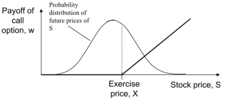
The payoff of a call option, w, on a non-dividend paying stock, S, is shown in Figure 2.§_{If the stock price, S, is less}

than the strike price, X, the option does not get exercised and the payoff is zero; however, if S is larger than X, the option holder has the option of buying the stock for X and then selling it for S, thus, making a profit of S – X. Mathematically, the payoff of a call option can be expressed as the maximum of S-X or zero, i.e., max[S-X, 0]. This profit must be compared to the cost of obtaining the option to determine the net profit.

(3)

American Institute of Aeronautics and Astronautics 3 Stock price, S Exercise price, X Payoff of call option, w

Figure 2: Payoff of a call option.

Options are said to be “in the money,” “at the money,” or “out of the money” depending on the cash flows that the option holder would obtain if the option would be exercised immediately.7_{If exercising the option results in positive}

cash flow, the option is “in the money;” if it results in a zero cash flow, it is “at the money;” and if it yields a negative cash flow, it is “out of the money.” For example, a call option is “in the money” if S > X, “at the money” if S = X, and “out of the money” if S < X.

Options are valuable because the future stock price is uncertain (see Figure 3). In fact, the value of an option increases with the volatility of the stock, because this means that the stock can reach higher prices (it can also reach lower prices, but we are not concerned about this because the option protects us from downside movements).

Stock price, S Exercise price, X Payoff of call option, w Probability distribution of future prices of S

Figure 3: The stochastic nature of stock prices make options valuable.

IV. Real Options Concepts

Real options analysis is based on financial options, but instead of purchasing or selling a financial asset, the owner of the real option can buy or sell a “real project.” A real option is basically a phased investment. Rather than spending all resources at the beginning of the project, the expenditures are divided such that an initial amount of resources are spent to explore the performance of the project. Once there is more information about the expected returns of the project, the full investment can be realized. For example, consider the development process of a new aircraft type, as shown in Figure 4:

Prelim. design

Product dev’t

Production Phase out

A C D E F

1.5 yrs 3 yrs 10 yrs 10 yrs

B Prelim. studies 0.5 yrs Prelim. design Product dev’t

Production Phase out

A C D E F

1.5 yrs 3 yrs 10 yrs 10 yrs

B

Prelim. studies

0.5 yrs

Figure 4: Main steps in a new aircraft development process.

Assume that a new aircraft model has passed the preliminary design phase and is waiting for approval from the board of directors to begin the product development stage. The development stage will provide the aircraft

(4)

manufacturer with a real option: at the end of development (Step D), management can decide whether to proceed with production and sales of the aircraft if it considers that the project will be successful. At that point, management will have a much better understanding of project costs and the potential revenues, thus, it will be able to make a much better decision than today. If the estimates are not positive, management may decide to cancel the project and avoid throwing resources into a failed project. The real options methodology proposed here will indicate management how much the real option is worth, i.e., how much money should be spent on the development phase. There are other real options embedded in the process shown in Figure 4. For example, in Step B, after the preliminary studies are completed, management has a real option to proceed with the preliminary design of the new aircraft model. During the product development period, there is a real option to abandon the project at each stage if development is not progressing at an acceptable rate. Finally, at Step D, there are several real options. One is the real option to produce the aircraft as described in the previous paragraph. Another real options is to sell the aircraft program to an interested buyer. A further real option is to launch a derivative version of the aircraft just developed. Finally, the investor has the real option to abandon the project.

V. Finding The Value Of The Real Option

A. Taxonomy of the real option to produce

In this paper, we are interested in the real option to produce the aircraft at point D. This is a European-like real option, because it can only be exercised at maturity. In addition, it is a call option, because by exercising, the option holder acquires the stock upon which the option is written. The elements of this real option are:

Stock price: The stock price is the present value of the expected income from aircraft sales throughout the life of the program. Here, income is defined as the difference of sales minus production costs. Aircraft production is estimated to last 10 years.

Strike price: The strike price is the present value of the cost of building the production facility, procuring tools and other non-recurring expenses associated with aircraft production. This is the expenditure that must occur in order to be able to acquire the stock.

Maturity: The time required to go from step C to step D is 3 years. Therefore, maturity for this real option is 3 years. At this point, the decision to produce aircraft or not must be made.

Value of the real option: The value of the real option is the maximum amount of money that should be assigned to develop the aircraft. These are the resources spent on the engineers to produce the final design and blueprints. It is customary to consider development cost as the sum of the engineers’ time and expenditures in production facilities; however, it is important to keep in mind the difference between them. Because of the existence of the real option, the decision to spend the money to build the production facilities can be postponed to the maturity date. At that time, management can decide to fully commit to aircraft production if conditions are favorable. The resources spent on the engineers’ time, however, must occur in order to obtain the real option to produce.

B. Evaluation of the real option

European call real options, like the one considered here, can be evaluated with the formula proposed by Miller and Clarke (2004) for real options where the stock price and the strike price are uncertain. This formula takes as inputs the probability distributions of the expected stock price, fs, and of the strike price, fx, and an appropriate discount

rate to calculate the expected value of the real option (see Equation 1):

_∫

=∞ −∞ = ⋅ = x x x x dx f x w x w E[ ( )] ( ) ( )

∫

∞ = ∞ = ∞ = ∞ =

⋅

−

⋅

=

x s s x x x s s x x

x

s

f

s

dsdx

x

f

x

f

s

dsdx

f

(

)

(

)

(

)

(

)

0 0 (Eq. 1)

(5)

In Equation 1, the distributions of the stock price and of the strike price are given in terms of their present values, i.e., they have already been discounted with the appropriate discount rate. The discount rate can be the one customarily used by the aircraft manufacturer to evaluate risky investments or it can be determined with the Capital Asset Pricing Model (CAPM), for example.

The distributions of strike price and stock price can be obtained with a combination of system dynamics and Monte Carlo simulation. System dynamics is a powerful simulation tool that models dynamic relationships between different components of a process or system. System dynamics can be combined with Monte Carlo simulation to take into account multiple sources of uncertainty and, thus, generate the probability distributions for the stock and for the strike prices.

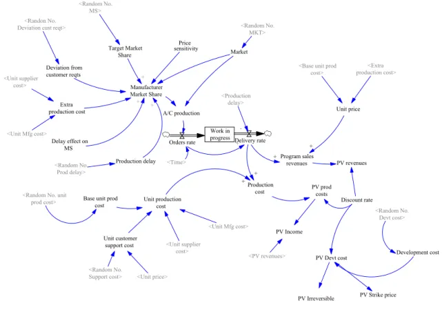
C. System dynamics model

A system dynamics model was developed with input from the aircraft manufacturer to determine the value of the real option to produce aircraft (see Figure 5). There are three main variables in this model: Manufacturer Market Share, Unit Production Costs and Unit Price. These are described below:

Manufacturer Market Share is key in this model because it determines the number of aircraft orders per year (Order rate). There are four variables that determine Manufacturer Market Share:

a) Target Market Share: This is an external variable that determines the maximum share of the total market for this particular aircraft that the manufacturer is expected to obtain. This parameter is uncertain because it depends on the actions by competitors. To capture this risk, a probability distribution for this variable is assigned in the Monte Carlos simulation (see below).

b) Production Delay: It has been estimated that 3 months of delay in the delivery of the aircraft has a negative impact of 0.5% on Manufacturer Market Share, i.e., for each 3 months of delay, Manufacturer Market Share decreases 0.5%.. As in the case of the Target Market Share, the amount of Production Delay is an uncertain parameter that can be accounted for in the Monte Carlo simulation.

c) Deviation from Customer Requirements: The product is developed to achieve a defined performance to satisfy customer needs. Each 1% of Deviation from customer requirements has a –1% impact on Manufacturer Market Share. This variable is also included in the Monte Carlo simulation as an exogenous variable.

d) Price sensitivity: This variable captures the negative impact of Unit Price increases on Manufacturer Market Share due to uncertain production costs. Unit Price is determined so that a certain margin over Base Unit Production Costs is achieved (see below); however, uncertainties in Unit Supplier Cost and Unit Manufacturing Cost can lead to Extra Unit Production Costs that are passed on to the aircraft buyers. Each $100,000 of Extra Production Costs results in a loss of 15 aircraft orders per year.

(6)

American Institute of Aeronautics and Astronautics 6 Work in progress Market Manufacturer Market Share Production delay Unit price Program sales revenues Unit production cost Unit customer support cost Production cost Delivery rate Orders rate Target Market Share Deviation from customer reqts + + + + Development cost <Time> <Production delay> -+ + Delay effect on MS + ₊ PV prod costs PV revenues PV Devt cost Discount rate PV Income <PV revenues> <Random No. MKT> <Random No. MS> <Random No. Prod delay> <Random No. Support cost> Extra

production cost A/C production

<Unit Mfg cost> <Unit supplier

cost>

<Random No. Devt cost> <Random No. unit

prod cost> Base unit prod_cost

Price sensitivity

PV Irreversible PV Strike price

<Unit price> <Randon No.

Deviation cust reqt>

Figure 5: System dynamics model to determine the value of the real option to produce aircraft. Unit Production Cost is the sum of the following variables:

a) Base Unit Production Cost: This is a random variable that is accounted for in Monte Carlo simulation b) Unit Customer Support Cost: Reflects costs due to warranties. This quantity is calculated as a random

percentage of Unit Price. This random percentage is included in the Monte Carlo simulation. c) Unit Supplier Cost: This is an uncertain quantity that is included in the Monte Carlo simulation. d) Unit Manufacturing Cost: This is also an uncertain quantity that is included in the Monte Carlo

simulation.

Unit Price is determined so that a certain margin over Base Unit Production Cost is achieved. In the base case, this margin is assumed to be 12%. If there are Extra Production Costs these are added on to Unit Price, which affect Price Sensitivity and Manufacturer Market Share as explained above.

Development Cost is an exogenous random variable that is calculated using the Monte Carlo simulation. It is an important quantity because it determines both the strike price and the Engineers’ Time. It is assumed that the strike price, i.e. the expenditures on the production facilities, are 20% of Development Costs. The remaining 80% is spend on the Engineers’ Time. Notice that this assumption could be relaxed to allow the strike price to be independent from Development Cost.

Order Rate is determined by Manufacturer Market Share and the size of the Market. Market is another exogenous variable with a probability distribution provided by the data from the aircraft manufacturer. It is assumed that all airplanes ordered in year n will be delivered in year n+1. Therefore, Delivery Rate is equal to Order rate. If Production delay is positive, aircraft are delivered in year n+1+Production delay.

(7)

Program Sales Revenues are obtained by multiplying Delivery Rate times Unit price. Production Costs is similarly the product of Delivery Rate times the Unit Production Cost. Income is the difference between Revenues and Production Costs. Using a suggested discount rate of 18% by the aircraft manufacturer, the present values of Income, Strike Price, Engineers’ Time and Development cost are calculated.

The model running time is in years. The first three years are for product development, only. Aircraft orders are first taken in the third year and aircraft delivers do not start until the fourth year. The simulation then runs for 12 years (it is assumed that production lasts only 10 years. The extra two years take into account delivery delays).

D. Monte Carlo simulation

Monte Carlo simulations can be run by specifying probability distribution for the exogenous variables of interest in the system dynamics model. The variables selected for this study and their associated probability distributions, as given by the aircraft manufacturer, are shown in Table 1:

Table 1: Variables selected for the Monte Carlo simulation and their associated probability distributions. Source: The authors with data from the aircraft manufacturer.

Variable Probability distribution

Unit Value P(value) Value P(value) Value P(value)

Market Aircraft/year 500 0.6 750 0.2 1000 0.2

Production Delay Year 1 0.6 0.75 0.2 0.5 0.2

Target Market Share % 20 0.5 30 0.3 40 0.2

Unit Production Cost US$ Million 2.4 0.6 2.3 0.3 2.2 0.1

Unit Customer Support Cost % of Unit price 5 0.5 4 0.4 3 0.1

Unit Supplier Cost US$ M/year 0.1 0.5 0.05 0.3 0 0.2

Unit Manufacturing Cost US$ M/year 0.1 0.5 0.05 0.3 0 0.2

Development Cost US$ Million 150 0.6 190 0.2 120 0.2

Deviation from Customer Requirement % 5 0.6 4 0.2 1 0.2

For this study, Market was assumed to take a value that remains constant throughout each simulation run. An alternative for introducing more realism into the simulation would be to assume a stochastic behavior of the aircraft market. This is a suggestion for future work.

VI. Numerical Results

A. Base case

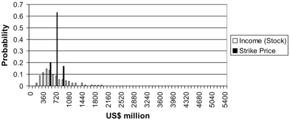
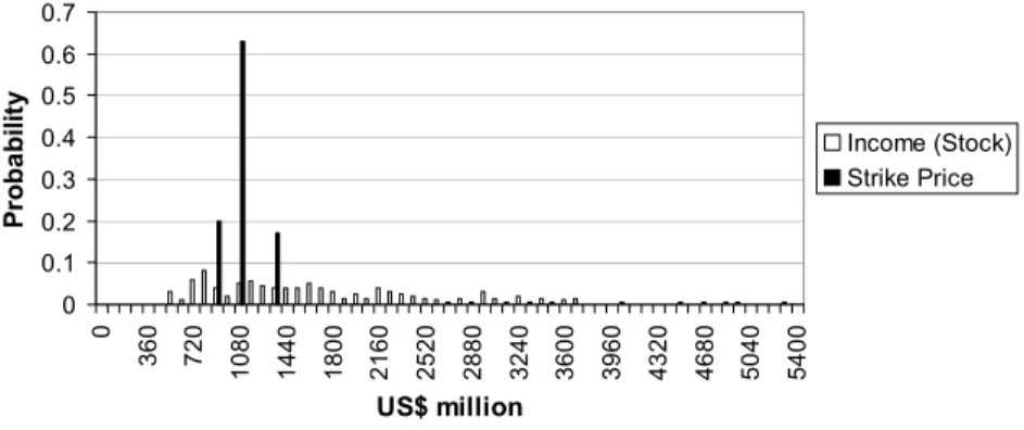
The probability distributions of the present values of Income and of Strike Price using the assumptions outlined above are shown in Figure 6. The stock price is between US$ 163.5 million and US$ 1,951.3 million. The range for the strike price is between US$ 245.4 million and US$ 375.1 million.

0 0.1 0.2 0.3 0.4 0.5 0.6 0.7 0 36 0 72 0 10 80 14 40 18 00 21 60 25 20 28 80 32 40 36 00 39 60 43 20 46 80 50 40 54 00 US$ million P ro b ab ilit y Income (Stock) Strike Price

Figure 6: Probability distribution of the present value of Income and of the Strike Price as determined by the Monte Carlo simulation in the base case.

(8)

A series of financial performance parameters for the aircraft program can be calculated with this data. These quantities are explained below and they are shown in Table 2:

• PV Income: present value of income, calculated directly from the Monte Carlo simulation

• PV Strike Price: present value of the strike price, calculated directly from the Monte Carlo simulation.

• Value Inflexible: this is the value of the strategy in which the real option to produce aircraft is always exercised at maturity regardless of the relative values of PV Income and PV Strike Price. Value Inflexible is the difference of PV Income minus PV strike price.

• Value Flexible: this is the value of the real option to produce aircraft. Here, the investor exercises the real option to produce aircraft at maturity only if PV Income is larger than PV Strike Price. This value is calculated substituting the probability distributions of PV Income and of PV Strike Price in Equation 1.

• PV Engineers’ Time: present value of expenditures on engineering and final design of the new airplane. This is calculated directly from the Monte Carlo simulation. This is the reference against which the value of the inflexible and flexible strategies should be compared.

• NPV Project: this is the result of subtracting PV Engineers’ Time from Value Inflexible or Value Flexible. This is the metric that management should consider when making the decision of investing in the project at all. • Value of flexibility: this is the difference between NPV Project Flexible and NPV Project Inflexible if both

strategies are implemented. It determines the relative value of the flexible strategy (the one that considers the real option) against the inflexible strategy (the one that always exercises at maturity). If NPV Project Inflexible is negative, this project would not be implemented and, thus, the Value of flexibility is equal to NPV Flexible. Table 2: Expected values (in US$ million) of different quantities of interest for the base case.

PV Income PV Strike Price Value Inflexible Value Flexible (Real Option)

PV Engineers’ Time NPV Project Value of flexibility Inflexible Flexible

634.64 302.42 332.22 339.61 1140.68 -808.46 -801.07 0.00

According to the results shown in Table 2, neither the Inflexible nor the Flexible strategies yield a positive NPV Project. Therefore, in this base case, the recommendation is not to buy the real option, which translates into not engaging into the development of the new aircraft.

It is important to indicate that the flexible strategy performs better than the inflexible strategy; however, the extra value that the flexible strategy provides is not enough to offset the cost of PV Engineers’ Time to yield a positive NPV Project. Thus, while a flexible strategy is preferred over an inflexible one, neither should actually be conducted. Therefore, the value of flexibility is zero.

Furthermore, notice that the initial investment in this real option, i.e. PV Engineers’ Time, is much larger than PV Strike Price. This is contrary to the usual situation in financial as well as in real options, where the amount of money to acquire the option (i.e., the option premium) tends to be considerably less than the strike price. This is an attractive feature of options, because it allows the option holder to wait and obtain more information before fully investing. Here, however, the option premium (i.e., PV Engineer’s Time) is much larger than the strike price. Therefore, there is little value in the ability to defer the investment because so much has already being spent before making the decision to fully invest or not. Thus, under these circumstances, a flexible strategy does not add enough value to make the project financially viable.

(9)

American Institute of Aeronautics and Astronautics 9 B. Case 2: Reducing the relative cost of Engineers’ Time and increasing Income

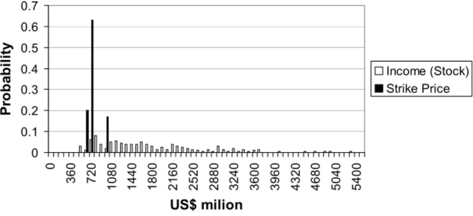
Management can resort to a number of alternatives to make the new aircraft project more attractive. Here, we consider two actions: first, Income is increased by specifying a margin of 25% above Unit Production Cost (this could be achieved, for example, by increasing price and/or decreasing Unit Production Cost); second, Development Costs are re-distributed so that the initial investment (i.e. Engineers’ Time) is only half of Development Costs, and the cost of the production facilities (i.e. the Strike Price) is the other half. This can represent a situation, for example, where some of the final design work is carried out in conjunction with the construction of the production facilities. The probability distributions of the present value of Income and of Strike Price using the assumptions outlined above are shown in Figure 7. In this case, Income is between US$ 455.5 million and US$ 5,261.4 million. The range for the strike price is between US$ 578.8 million and US$ 903.1 million.

0 0.1 0.2 0.3 0.4 0.5 0.6 0.7 0 360 720 ₁₀₈₀ ₁₄₄₀ ₁₈₀₀ ₂₁₆₀ ₂₅₂₀ ₂₈₈₀ ₃₂₄₀ ₃₆₀₀ ₃₉₆₀ ₄₃₂₀ ₄₆₈₀ ₅₀₄₀ ₅₄₀₀ US$ milion P roba bilit y Income (Stock) Strike Price

Figure 7: Probability distribution of the present value of Income and of the Strike Price as determined by the Monte Carlo simulation with the assumptions of Case 2.

The expected value of the quantities of interest with the assumptions of Case 2 are given in Table 3. The results are more favorable to investment in the real option than in the base case. Now, both the Inflexible and Flexible strategies yield a positive Project NPV of US$285.37 million and US$299.17 million, respectively. Thus, in this scenario, management should proceed with purchasing the real option to produce the aircraft by investing PV Engineers’ Time in the final development of the aircraft. Notice that the value of the flexible strategy over the inflexible strategy is relatively small (US$13.80 million). Here, because the strike price is small compared to the stock price, the real option is exercised very frequently. Therefore, the flexible strategy is exercises the real option almost as often as in the inflexible case.

Table 3: Expected values (in US$ million) of different quantities of interest where Engineers’ Time is 50% of Development Cost and PV Strike Price is the remaining 50%. Income is increased by establishing a 25% margin of Unit Price over Unit Production Cost.

PV

Income PV Strike Price Inflexible Value Value Flexible (Real Option) PV Engineers’ Time NPV Project flexibility Value of Inflexible Flexible

1728.47 721.55 1006.92 1020.72 721.55 285.37 299.17 13.80

C. Case 3: Further reduction of relative cost of Engineers’ Time

In order to illustrate when the flexible strategy, i.e. the real option, can be key to determine the fate of the project, consider that the Strike Price increases by approximately 30%. Development Cost and PV Engineers’ Time are the same as in Case 2. Income is still calculated by assuming a 25% margin over Unit Production Cost. The probability distributions of income and of stock price with these assumptions are shown in Figure 8. Income is between US$ 455.5 million and US$ 5,261.4 million, as in Case 2, but the range for the strike price is now between US$ 856.8 million and US$ 1,343.2 million.

(10)

American Institute of Aeronautics and Astronautics 10 0 0.1 0.2 0.3 0.4 0.5 0.6 0.7 0 360 720 ₁080 ₁440 ₁800 ₂160 ₂520 ₂880 ₃240 ₃600 ₃960 ₄320 ₄680 ₅040 ₅400 US$ million Pr o b a b ilit y Income (Stock) Strike Price

Figure 8: Probability distribution of the present value of Income and of the Strike Price as determined by the Monte Carlo simulation with the assumptions of Case 3.

The expected value of the quantities of interest are given in Table 4:

Table 4: Expected values (in US$ million) of different quantities of interest for the case where Strike Price increases by approximately 30%. Engineers’ Time, Development cost and Income are the same as in Case 2.

PV Income PV Strike Price Value Inflexible Value Flexible (Real Option)

PV Engineers’ Time NPV Project Value of flexibility Inflexible Flexible

1728.47 1070.82 657.64 745.53 721.55 -63.90 24.98 24.98

The inflexible strategy results in a negative project NPV and should not be implemented. On the contrary, the flexible strategy provides investors the real option of not fully investing at maturity if PV Strike Price is less than PV Income. Here, the strike price is larger than in Case 2, thus, the ability not to fully invest becomes very valuable. In fact, the presence of the real option leads to an expected project NPV of US$24.98 million for the flexible case. Thus, the value of flexibility is also US$24.98 million. This result indicates that management should purchase the real option to produce aircraft only if it adopts the flexible strategy.

A flexible strategy is generally more costly than an inflexible one because there may be expenditures associated with providing the flexibility. In this particular case, an example of an extra cost could be a premium paid in advance to compensate the hangar construction company in case the real option is not exercised at maturity. According to the results in Table 4, the aircraft manufacturer should pay no more than US$ 24.98 million for these extra costs.

VII. Conclusion

The methodology presented in this paper uses real options analysis and Monte Carlo simulation to evaluate flexible investment decisions in air transportation. The methodology is illustrated by analyzing a new aircraft development program. According to the assumptions in the baseline scenario, the real option to produce aircraft is not very valuable. In this particular application, unlike typical financial or real options, the option premium is much larger than the strike price. Therefore, there is little value in the ability to defer the investment because so much has already being spent before making the decision to fully invest or not.

This indicates at least two possible ways forward. First, there may still be opportunity to improve the financial performance of the aircraft production program. Clearly, increasing revenues by specifying a higher margin over Unit Production Cost will make the project financially more attractive. Another possibility is to shift expenditures so that more investment occurs at maturity of the real option and not before. In this way, the ability not to invest becomes more valuable as not so many resources would have already being spent. A second way forward would be to look for other points earlier in the aircraft development process where the real options may be more valuable. For example, the real option to engage in product development after the preliminary design has been completed (Step C)

(11)

is a good candidate. The amount of resources spent on the preliminary design are likely to be small compared to the development expenditures. Thus, the real option that exists at Step C may be very valuable.

Bibliography

1_{Skinner, Steve, Alex Dichter, Paul Langley and Hendrik Sabert (1999) “Managing Growth and Profitability across}

Peaks and Troughs of the Airline Industry Cycle – An Industry Dynamics Approach,” G. Butler and M. Keller eds. Handbook of Airline Finance. MacGraw-Hill, New York.

2_{Stonier, John E. (1999) “What is an Aircraft Purchase Option Worth? Quantifying Asset Flexibility Created through}

Manufacturer Lead-Time Reductions and Product Commonality.” G. Butler and M. Keller eds. Handbook of Airline Finance. MacGraw-Hill, New York.

3_{Air Transportation Association (2004) “Annual Traffic and Capacity: US airlines – scheduled traffic.” Available at:}

http://www.airlines.org/econ/ [cited 10 June 2004].

4_{Bureau of Economic Analysis (2004) “Current-Dollar and “Real” Gross Domestic Product.” Available at:}

http://www.bea.doc.gov/bea/dn/gdplev.xls [cited 10 June 2004]

5_{Black, Fischer and Myron Scholes. “The Pricing of Options and Corporate Liabilities,” Journal of Political Economy.}

Vol. 81, 1973.

6_{Brealey, Richard A. and Stewart C. Myers (1996) Principles of Corporate Finance. 5}th_{Edition. McGraw-Hill, New} York.

7_{Hull, John (1995) Introduction to Futures and Options Markets. New Jersey: Prentice Hall. 2}nd_Edition.

8_{Miller, Bruno and John-Paul Clarke (2004) Investments Under Uncertainty in Air Transportation: A Real Options}

Perspective. Presented at the 45th_{Annual Forum of the Transportation Research Forum (TRF), Evanston, Illinois.} Submitted for publication.