Changes in Stratospheric Temperatures and Their Implications
for Changes in the Brewer–Dobson Circulation, 1979–2005
The MIT Faculty has made this article openly available.
Please share
how this access benefits you. Your story matters.
Citation
Young, Paul J., et al. “Changes in Stratospheric Temperatures and
Their Implications for Changes in the Brewer–Dobson Circulation,
1979–2005.” Journal of Climate, vol. 25, no. 5, Mar. 2012, pp. 1759–
72.
As Published
http://dx.doi.org/10.1175/2011JCLI4048.1
Publisher
American Meteorological Society
Version
Final published version
Citable link
http://hdl.handle.net/1721.1/118404
Terms of Use
Article is made available in accordance with the publisher's
policy and may be subject to US copyright law. Please refer to the
publisher's site for terms of use.
Changes in Stratospheric Temperatures and Their Implications for Changes
in the Brewer–Dobson Circulation, 1979–2005
PAULJ. YOUNG,* KARENH. ROSENLOF,1SUSANSOLOMON,#STEVENC. SHERWOOD,@ QIANGFU,&ANDJEAN-FRANCxOISLAMARQUE**
* Cooperative Institute for Research in the Environmental Sciences, University of Colorado, and National Oceanic and Atmospheric Administration, Boulder, Colorado
1National Oceanic and Atmospheric Administration, Boulder, Colorado
#Department of Atmospheric and Oceanic Sciences, University of Colorado, Boulder, Colorado @University of New South Wales, Sydney, Australia
&University of Washington, Seattle, Washington
** National Center for Atmospheric Research, Boulder, Colorado (Manuscript received 2 September 2010, in final form 1 August 2011)
ABSTRACT
Seasonally and vertically resolved changes in the strength of the Brewer–Dobson circulation (BDC) were inferred using temperatures measured by the Microwave Sounding Unit (MSU), Stratospheric Sounding Unit (SSU), and radiosondes.
Linear trends in an empirically derived ‘‘BDC index’’ (extratropical minus tropical temperatures), over 1979–2005, were found to be consistent with a significant strengthening of the Northern Hemisphere (NH) branch of the BDC during December throughout the depth of the stratosphere. Trends in the same index suggest a significant strengthening of the Southern Hemisphere branch of the BDC during August through to the midstratosphere, as well as a significant weakening during March in the NH lower stratosphere. Such trends, however, are only significant if it is assumed that interannual variability due to the BDC can be removed by regression of the tropics against the extratropics and vice versa (i.e., exploiting the out-of-phase nature of tropical and extratropical temperatures as demonstrated by previous studies of temperature and the BDC).
The possibility that the apparent lower-stratosphere BDC December strengthening and March weakening could point to a change in the seasonal cycle of the circulation is also explored. The differences between a 1979–91 average and 1995–2005 average tropical temperature seasonal cycle in lower-stratospheric MSU data show an apparent shift in the minimum from February to January, consistent with a change in the timing of the maximum wave driving. Additionally, the importance of decadal variability in shaping the overall trends is highlighted, in particular for the suggested March BDC weakening, which may now be strengthening from a minimum in the 1990s.
1. Introduction
The Brewer–Dobson circulation (BDC) describes the time-mean, Lagrangian mean meridional mass flux that links the tropics to the extratropics in the stratosphere (Dunkerton 1978). A future strengthening of this circu-lation in response to increases in greenhouse gas con-centrations is a robust result of stratospheric models (e.g., Butchart et al. 2006, 2010), meaning that observed changes may provide a fingerprint of anthropogenic cli-mate forcing. A change in the strength of the BDC would
also impact the concentration of water vapor (Randel et al. 2006; Rosenlof and Reid 2008) and the transport of ozone (Randel et al. 2002b) and ozone-depleting chem-icals (Butchart and Scaife 2001), with related impacts on the tropospheric ozone budget (Sudo et al. 2003) and surface UV index (Hegglin and Shepherd 2009), and would coincide with changes in the dynamics and tem-perature of the stratosphere (Lin et al. 2009). Here, temperature data from the satellite-borne Microwave Sounding Unit (MSU) and Stratospheric Sounding Unit (SSU), together with radiosondes, are examined for evi-dence of changes in the BDC over 1979–2005. Advantage is taken of well-established relationships between tropical and winter/spring hemisphere extratropical temperature anomalies and interannual variation in the circulation’s
Corresponding author address: Paul Young, NOAA/ESRL, 325 Broadway R/CSD8, Boulder, CO 80305.
E-mail: paul.j.young@noaa.gov DOI: 10.1175/2011JCLI4048.1
strength, which have been previously demonstrated for the lower (Ueyama and Wallace 2010) and middle and upper (Young et al. 2011) stratosphere.
The poleward transport of the BDC is forced through wave momentum deposition and is stronger in the winter and spring seasons in both hemispheres (Haynes et al. 1991; Holton et al. 1995; Rosenlof 1995; Fueglistaler et al. 2009); it generally reaches a maximum during Northern Hemisphere (NH) winter. The circulation is upward in the tropics and downward at mid- to high latitudes, driving temperatures respectively cooler and warmer than their radiative equilibrium values (e.g., Shine 1987). Yulaeva et al. (1994) documented the temperature signal of the BDC in the lower stratosphere using MSU data, and the approach was extended to the middle and upper stratosphere, using SSU data, by Young et al. (2011). Both studies showed that tropical temperature anomalies are significantly anticorrelated with the extratropics of the winter/spring hemisphere, consistent with inter-annual changes in strength of the BDC, that is, anom-alous cooling (warming) in the tropics and anomanom-alous warming (cooling) in the extratropics if the circulation is stronger (weaker) than average (see also Fritz and Soules 1972; Randel et al. 2002a; Thompson and Solomon 2005; Ueyama and Wallace 2010). Here, this empirical pattern is exploited to look for the presence of out-of-phase temperature trends, which could indicate trends in the BDC. However, it is noted that the satellite data only span a few decades and hence are probably insuf-ficient to allow discrimination between decadal variabil-ity and longer-term systematic changes. Nevertheless, it is useful to test whether changes emerge for the pe-riod of record.
Lower-stratosphere temperature data from the MSU instrument have previously been analyzed for changes in the BDC. While annual mean trends have been shown to be consistent with a strengthening of the BDC (Thompson and Solomon 2009), other studies have examined the seasonality of the trends. Hu and Fu (2009) used the MSU data to show significant and strong 1979–2006 warming trends of 5–8 K located off the Pole in the Southern Hemisphere (SH) high latitudes, for the months of September and October. This warming is accompanied by a slightly weaker widespread cooling trend, also off-pole, imparting a wavenumber-1 spatial pattern (Hu and Fu 2009; Lin et al. 2009) and resulting in a reduced SH warming in the zonal mean (see Ramaswamy et al. 2001; Randel et al. 2009). A regression analysis by Lin et al. (2009) used eddy heat fluxes from reanalysis data to suggest that the observed SH September trend pattern is consistent with an increase in the strength of the BDC driving the heating and ozone depletion driving the cooling.
Northern Hemisphere high-latitude wintertime (De-cember and January) warming over the past three decades is evident in the zonal mean MSU lower-stratosphere trends (Randel et al. 2009), which Fu et al. (2010, here-after FSL10) showed to coincide with tropical cooling trends and therefore potentially signal an increase in the BDC strength. FSL10 also noted a NH high-latitude cooling trend during March, coincident with tropical warming, which was interpreted as further evidence for a weakening NH cell of the BDC in that season (see also Randel et al. 2002a). Free (2011) showed that these seasonal and spatial patterns in lower-stratosphere tem-perature trends are robust in several different radio-sonde datasets, although cautioned that the apparent trends could reflect decadal variability.
Most model studies suggest a strengthening of the BDC in the lower stratosphere over the latter half of the twentieth century, based on changes in quantities such as 70-hPa tropical vertical velocities or mass fluxes (e.g., Garny et al. 2007; Olsen et al. 2007; Li et al. 2008; Garcia and Randel 2008; McLandress and Shepherd 2009; Lamarque and Solomon 2010). These increases have been ascribed to enhanced driving from waves originating in the troposphere, coupled with changes in vertical wave propagation, refraction, and dissipation forced by shifts in stratospheric winds and temperatures (e.g., Eichelberger and Hartmann 2005; Butchart et al. 2006, 2010; Olsen et al. 2007; Garcia and Randel 2008). It may be that the contribution of different types of waves (resolved vs parameterized) are different depending on the model (Garcia and Randel 2008; McLandress and Shepherd 2009), although some differences may be due to the lat-itude bands chosen for averaging the trends (McLandress and Shepherd 2009). Where the seasonal variation is discussed, several model studies (Butchart and Scaife 2001; Butchart et al. 2006; Li et al. 2008; Garny et al. 2009; McLandress and Shepherd 2009) report that their maximum trends are observed during boreal winter, in the December–February (DJF) season. Li et al. (2008), Garny et al. (2009), and McLandress and Shepherd (2009) all suggest that the impact of austral spring ozone depletion on wave propagation results in a stronger SH branch of the BDC during DJF. In terms of vertically resolved changes, Li et al. (2008) report stronger trends in the lower stratosphere, although Garcia and Randel (2008) report maximum trends in both the lower and upper stratosphere. The present study will use the MSU and SSU data to probe whether there is evidence of ver-tical and seasonal patterns of BDC changes.
In contrast to the model results and temperature anal-yses, some studies using tracer data have argued against changes in BDC strength. For instance, Cook and Roscoe (2009) concluded that there was no significant trend in
BDC strength using NOy measurements made over Antarctica since 1990. An analysis of stratospheric age-of-air trends from measurements of sulfur hexafluoride (SF6) and CO2mixing ratios was interpreted to suggest that there has been no significant trend in the BDC over the past three decades, although an increase in lower-stratospheric tropics-to-pole transport could not be ruled out (Engel et al. 2009). Ray et al. (2010) conducted fur-ther analysis of the age-of-air dataset, in tandem with modeling, and concluded that the observations are best matched by a strengthening of the lower-stratospheric circulation, coupled with a weakening of the circulation in the middle and upper stratosphere and an increase in horizontal mixing between the tropics and midlatitudes. This result highlights the importance of better estimating height-resolved changes in the BDC.
The present work builds on the MSU lower-stratospheric trends studied by FSL10 by using tem-peratures from independent datasets (i.e., the SSU instrument and radiosondes, which together provide information on higher altitudes), covering most of the depth of the stratosphere. While it is noted that tem-perature data are not perfect indicators of long-term changes in BDC strength, the relatively long observa-tional record affords a seasonally and vertically resolved analysis not possible with composition data (e.g., Engel et al. 2009; Ray et al. 2010).
This study is organized as follows. Section 2 describes the MSU, SSU, and radiosonde temperature data, to-gether with information on how linear trends and their statistics were calculated. General features of the sea-sonal cycle for the zonal mean and global, tropical, and extratropical mean changes (over 1979–2005) are pre-sented in section 3. In section 4, differences in tropical and extratropical temperatures are used to define a BDC index, which is analyzed for secular trends in BDC strength. The main conclusions are summarized in section 5.
2. Temperature data and trend calculations a. Satellite brightness temperature data
Satellite temperature data are from the lower-stratospheric channel of the MSU instrument (MSU TLS), and the middle- (SSU-25, SSU-26) and upper-(SSU-27) stratospheric channels of the SSU instru-ment. Table 1 summarizes the approximate peaks and half-power widths of the weighting functions (see also Young et al. 2011, their Fig. 1). Note that the MSU TLS weighting function spans a relatively thick atmospheric layer, the lower altitude end of which includes part of the tropical upper troposphere.
Zonal mean, monthly mean brightness temperature datasets for SSU data were provided as anomalies (rel-ative to a 1980–94 monthly mean climatology) by the NOAA Climate Prediction Center (C. Long and R. Lin 2009, personal communication). The data cover the years 1979–2005 and span 708S–708N with a resolution of 108. They include diurnal and semidiurnal tidal corrections, as well as a correction to the weighting functions to account for the increase in atmospheric CO2concentration since 1979 (see Shine et al. 2008; Randel et al. 2009). The data were used in a recent assessment of stratospheric tem-perature trends (Randel et al. 2009). Note that these SSU data have missing values in May, June, and December 1995. Additionally, the SSU-26 data are missing for July and August 1984, and the SSU-27 data are missing for January–July 1979 and April 1980.
Lower-stratospheric temperatures are from version 3.2 of the MSU-TLS data from the Remote Sensing Systems (RSS) ( Mears and Wentz 2009). The time series consists of a combination of channel 4 from the MSU and channel 9 from the advanced MSU (AMSU) instruments. Zonal and monthly mean data covering 1979–2005 (for consis-tency with the SSU data) are used in this study, spanning 82.58S–82.58N with a resolution of 2.58.
Discussion of potential error sources in the MSU and SSU data can be found in Randel et al. (2009, and ref-erences therein). For the purpose of trend calculations, the most significant sources of error are likely from combining the results of individual MSU and SSU in-struments across different satellites to construct the time series. However, the focus here is on patterns of change, especially high latitude 2 tropical differences, which should be less affected by such errors than absolute trends (assuming that satellite offsets are not different for different latitudes).
b. Radiosonde data
Analysis of the satellite temperature data was supple-mented with radiosonde temperatures from the Iterative Universal Kriging (IUK) radiosonde dataset (Sherwood et al. 2008), available at pressures ranging from 850 to 30 hPa for the period 1958–2005. The temperatures were homogenized using an iterative process that converges to a maximum-likelihood estimate of trends, change points,
TABLE1. Approximate weighting function peaks and half-power ranges for the MSU and SSU channels.
Channel Peak Half-power range
SSU-27 1.5 hPa (45 km) 5–0.4 hPa (36–55 km)
SSU-26 3 hPa (39 km) 15–1 hPa (28–48 km)
SSU-25 10 hPa (31 km) 40–3 hPa (22–39 km)
and missing values using twice-daily operational radio-sonde data. While it is unlikely that any homogenization effort will be perfectly successful, in simple statistical simulations this approach yields more accurate climate changes than common approaches to the problems of missing data and bias heterogeneity (Sherwood 2007). This method estimates bias changes independently for each of four seasons, unlike other radiosonde homoge-nization efforts. This is important since bias changes are likely to depend on solar zenith angle and mean tem-perature, particularly helpful for polar regions, which are relevant in this study. However, it is noted that bias changes in the radiosondes and missing data can be significant at stratospheric levels.
For comparison with the satellite data, this study uses radiosonde data at 30 hPa (the highest level), as well as temperatures weighted with the MSU TLS weighting function. Zonal mean temperatures were constructed by binning the 460 stations with twice-daily data (‘‘A’’ stations, Sherwood et al. 2008) into 108-wide latitude bands.
c. Linear trend calculations
Trends were calculated using linear least squares re-gression on data binned by month. Statistical uncer-tainties in the linear fits for the satellite data are assessed using the technique outlined by Santer et al. (2000), accounting for serial autocorrelation through adjust-ment of the effective sample size n, which is then used to calculate the standard error (s) for the slope. Uncer-tainties are then quoted with either 61s (’68% confi-dence) or 62s (’95% conficonfi-dence) limits. Note that the quoted uncertainties are statistical, do not include sys-tematic errors in the temperature data, and are esti-mated independently for each calendar month.
3. Seasonal patterns of temperature trends, 1979–2005
We will first consider the latitudinal and seasonal struc-ture of the raw temperastruc-ture trends. The goal here is to document the seasonal and latitudinal patterns of tem-perature changes, to identify whether there are tropical– extratropical trend relationships that are consistent with significant changes in the BDC over the 27-yr data re-cord (i.e., out-of-phase trends), and to note whether there are particular months and altitudes that display stronger signals. These results build on similar ones presented for the MSU-TLS data by FSL10. Note, for ease of de-scription, the term ‘‘trend’’ is used throughout to describe the regression coefficient obtained from the linear re-gression against time, and, if the trend is significant, this is stated in the text.
a. Zonal mean temperature trends: Satellites and radiosondes
Figure 1a shows the temperature trends for the MSU and SSU data as a function of month and latitude, with the contours filled only where the trend is significantly different from zero at the 2s level. Figure 1b shows comparable lower-stratosphere trends from radiosonde data. The bottom panel presents trends from MSU TLS weighted radiosonde data and the top panel is from the radiosonde data at 30 hPa, providing a comparison to an independent set of observations. The 30-hPa pressure level is the highest altitude in the homogenized radio-sonde database, and positioned roughly midway between the MSU TLS and SSU-25 weighting functions (Table 1). In general, the patterns of monthly and latitudinal trends from the radiosonde dataset match remarkably closely those for the MSU TLS and SSU-25 data, although the patterns are noisier due to more spatially limited radio-sonde coverage. The cooling in the tropics also appears somewhat enhanced relative to the satellite data. The MSU TLS panel of Fig. 1a is very similar to that pre-sented for the 1980–2008 trends for the RSS data dis-cussed by FSL10, as well as for the trends derived from alternative temperature retrieval conducted by the Uni-versity of Alabama (Christy et al. 2003) shown by Randel et al. (2009; their Fig. 11a).
While the MSU and SSU-25 and -26 data show ab-solute warming at high latitudes during the respective winter seasons, potentially reflecting an increase in BDC strength, the trends are not significant. It is notable that both hemispheres display maximum changes in the winter– spring months, consistent with the timing of strongest planetary wave driving. Figure 1a shows that the warming peaks at ;2 K decade21 during January and 0.5–0.8 K decade21during September for MSU TLS, and is up to 0.5 K decade21for SSU-25 and -26 in December and August. From Fig. 1b, NH December–January high-latitude warming in the radiosonde data is smaller in both magnitude (1.5 K decade21) and latitudinal extent (to ;608 vs ;508N) compared to the satellite trends.
While the austral spring SH high-latitude warming is not significant at either the 1s or 2s level in either the MSU TLS or radiosonde dataset, it is common to both. Furthermore, we know that from August to November the lower-stratosphere warming pattern is zonally asym-metric (e.g., Hu and Fu 2009; Lin et al. 2009; FSL10), which would dilute the magnitude of the zonal mean trend. Trends in reanalysis data, determined by Hu and Fu (2009), suggest that a zonally asymmetric September warming occurs from 100 to 20 hPa. Therefore, it is con-ceivable that the observed weak zonal mean warming for the SSU data in Fig. 1 is also related to an asymmetric
FIG. 1. (a) Latitude–month plots of (a) the linear trend of the MSU and SSU data and (b) the linear trend of the MSU TLS-weighted and 30-hPa radiosonde temperature data (in between MSU TLS and SSU-25). Pressure values (as in subsequent figures) indicate the approximate peak of the weighting function. Color-filled contours indicate where the trends are significant at the 2s level. The zero trend line is indicated by a thick contour.
pattern of warming and cooling. (Unfortunately, these SSU data are only available as zonal averages so it was not possible to analyze zonal asymmetries.)
In addition to zonal asymmetries in the warming trend, strong radiative cooling from ozone depletion in October and November (e.g., Randel and Wu 1999) will also serve to negate any warming due to enhanced descent when viewed in the zonal mean (Lin et al. 2009; FSL10). MSU TLS data in Fig. 1a suggests that the ozone depletion results in a near-zero SH high-latitude zonal mean trend in October, followed by a significant 21.5 K decade21 cooling trend during November–December (where the cooling overwhelms any zonally asymmetric dynamical warming). Note that maximum ozone depletion is located from 15 to 20 km (Solomon 1999), around the center of the MSU TLS weighting function (Table 1). Figure 1b shows that the ozone-related cooling in austral spring starts a month earlier in the radiosonde data and is more than 50% greater in magnitude, which could be due to sampling biases toward certain longitudes.
Zonal asymmetries are also important for the case of the MSU December trends in northern high latitudes (FSL10). Warming patterns for NH high latitudes aloft are most evident in December, but are not statistically significant compared to the large interannual variability in that season. In contrast, FSL10 showed that trends for January were more zonally symmetric, and the January warming in the MSU TLS data and the MSU TLS-weighted radiosonde data are the only absolute warming trends significant at the 1s level.
While Fig. 1a shows that the trends at the SSU-27 level are generally all significant (except for the NH high lati-tudes in winter), the latitudinal trend patterns seen in the other data are not as clear. The SSU-27 level is charac-terized by a year-round minimum in the cooling trend centered around 408S and 408N, as also noted by Randel et al. (2009). This relative warming becomes more notable during the winter months in each hemisphere, although it is displaced equatorward and is less clear of a continuation of the BDC-like signal in the other channels.
Figure 1 also shows the lower-stratosphere (MSU TLS level and SSU-25) high-latitude cooling in NH spring, which is significant at the 1s level. The cooling peaks at .1.5 K decade21 poleward of 708N during March for MSU TLS, and it is paired with a small, but not signi-ficant, warming in tropical latitudes. While part of the high-latitude cooling may be attributed to springtime ozone depletion, note that the NH ozone loss is less than that experienced in the SH and less radiative cooling would be expected (Randel and Wu 1999; Solomon 1999). The fact that the magnitude of the NH cooling is comparable to that during late spring in the SH is
consistent with an additional (negative) dynamical forc-ing. Furthermore, it is interesting to note that the March zonal mean tropical warming at the MSU TLS level is the result of a zonally asymmetric pattern being driven by a significant warming trend situated over the central tropical Pacific (maximum ;58–358N). At the tropopause level, temperatures in this region are important for con-trolling the concentration of stratospheric water vapor (Rosenlof and Reid 2008).
b. Seasonal patterns and relationship of the tropical and extratropical trends
We will next look at trends averaged by latitude band, which dampens interannual variability increasing the signal/noise ratio. For the following discussion, the tropics are defined as the 208S–208N average, and the extratropics the average poleward of 408, which is the same as that used by FSL10. Moreover, analysis of the interannual relationship of tropical and extratropical temperatures for MSU and SSU data by Young et al. (2011) showed that the winter–spring hemisphere latitudes poleward of ;408 display a significant out-of-phase relationship with 208N/S-averaged temperatures, consistent with these re-gions reflecting the tropical upwelling and extratropical downwelling of the BDC (see also section 4). ‘‘Global’’ averages refer to the full extent of the available data: 708N/S for the SSU temperatures and 82.58N/S for the MSU TLS temperatures.
Figure 2a shows the trends by month for the tropical, NH and SH extratropics, and global averages for the MSU and SSU data. Note the change in the y-axis scale between the different panels for this figure and that the time axis runs from June to May. Whether a trend is significantly different from zero is indicated by symbols on the plot: crosses for significance at the 1s level and circles for significance at the 2s level. Radiosonde TLS trends (not shown) agree well with MSU TLS in terms of the seasonal cycle (r 5 0.89–0.96 for each latitude band), although their values are generally lower. This is espe-cially the case for the SH spring/ozone hole period, as noted above, which has up to 0.6 K decade21more cooling in the radiosonde data. Maximum differences for other latitude bands are 0.1–0.2 K decade21more cooling in the radiosondes, except for the December NH where the MSU trend is 10.4 K decade21(see below) and the ra-diosonde trend is zero.
Figure 2a indicates that global mean cooling trends are apparent for all channels, which modeling studies suggest are driven by a combination of increased con-centrations of greenhouse gases (including water vapor) and ozone depletion (e.g., Shine et al. 2003). Global mean trends are significant at the 2s level year-round for SSU-27, SSU-25, and MSU TLS data. The same level
FIG. 2. (a) Trends by month of the global (full extent of data, solid), NH (.408N, dashed), and SH (.408S, dash– dotted) extratropical and tropical (208S–208N, dotted) average temperatures for the MSU and SSU data. Symbols indicate trends significantly different from zero at the 1s (crosses) or 2s level (circles). (b) Trends by month of the NH and SH extratropical average (dashed) and tropics (dotted) minus the global mean trend. The correlation be-tween the tropical and extratropical average trends is shown in each panel. Cross symbols indicate where the trend is significantly different from the global mean trend at the 1s level (no 2s significant trends). Note that the month coordinate starts at June.
of significance is only apparent for seven months in the SSU-26 data, where 1s significant trends are seen during May, June, August, September, and November. Annual mean trends are approximately 20.3, 20.5, 20.4, and 21.2 K decade21for MSU TLS, SSU-25, SSU-26, and SSU-27, respectively, in close agreement with the trends presented by Randel et al. (2009, their Fig. 19), which were calculated using multiple linear regression. [See Randel et al. (2009) for further review of the overall temperature trends.]
Seasonal variation of the temperature trends is also clear from Fig. 2a, most notably for the NH and SH ex-tratropics. From MSU TLS to SSU-27 there is a warming trend for the NH extratropics in December (December– January for MSU TLS), and for the SH extratropics in August (August–September for MSU TLS), compared to the other months. This pattern is clearer in the lat-itudinal averages compared to Fig. 1. Furthermore, it appears that the relative magnitude of the August SH trend, as compared to the December NH trend, decreases with altitude. However, note that the SH warming in August is only significant (2s) in the SSU-27 data, and the NH warming in December is only significant (1s) in the MSU TLS data.
The radiative impact due to ozone depletion is also clear in Fig. 2a, with the MSU TLS SH extratropics showing a negative trend that starts after September and bottoms out in December (where it is significant at the 2s level). Additionally, as noted above, tempera-ture trends for the NH extratropics of the MSU TLS data show a clear and significant minimum in March, with the SSU-25 and -26 data showing a minimum in February.
Inspection of Fig. 2a suggests that the SH and NH positive trends in August and December, respectively, are generally coincident with enhanced tropical cooling, consistent with a strengthening of the BDC (FSL10). Furthermore, the February–March NH cooling is co-incident with tropical warming, consistent with the BDC weakening. The changes in the tropical temperatures are smaller in magnitude than those at high latitudes, which would be expected for a BDC signal based on the area weighting of the upwelling and downwelling regions (see also Fritz and Soules 1972; Young et al. 2011). Correla-tions of the annual cycle of the SSU trends with those of MSU TLS suggest similar annual variations in extra-tropical and extra-tropical trends from MSU TLS to SSU-26, consistent with coherent drivers of the trends from the lower to midstratosphere. At the SSU-27 level, only the tropical trends are still significantly correlated with MSU TLS.
Figure 2b shows the pairing of the tropical and extra-tropical trends more clearly by expressing them as anom-alies relative to the global mean trend. In this figure, the
NH and SH high latitudes are averaged together, some-what canceling the strong cooling imparted by the ozone hole in the SH data. Symbols here indicate where the tropical or extratropical trend is significantly different (at only the 1s level) from the global mean, determined from the trend in the difference between the tropical or extratropical mean temperatures and the global mean temperature.
Removal of the global mean trend can be considered as a rough proxy for removing the cooling due to in-creases in the concentrations of well-mixed greenhouse gases, assuming that this effect has been globally uni-form. As such, we are left with anomalies that include the effects of dynamical changes, but also any latitudinal gradients in temperature trends, for example, as caused by ozone depletion or other forcings, such as water va-por trends. Despite such limitations, the correlations be-tween the tropical and extratropical trends (as indicated in Fig. 1b) clearly show that the annual cycle of trends are significantly anticorrelated at all levels, consistent with seasonal changes in the strength of the BDC strongly influencing the seasonal trends throughout the strato-sphere (i.e., as per FSL10, who showed this in a similar manner for the MSU-TLS data). However, we note that few of the trends are significantly different from the global mean trend, and then only at the 1s level.
The issue of significance is what motivates examina-tion of the out-of-phase nature of the tropical and extra-tropical temperatures to explore potential trends in a different manner, that is, one that reduces the noise from interannual variability. An example of such a method is explored in the next section.
4. A temperature-related index of BDC strength? Section 3 documented that the temperature trends show patterns consistent with possible BDC changes, but the lack of statistical significance for most of the individual trends for particular latitudes in isolation meant that nothing definitive could be said about a trend in BDC strength from raw temperatures alone. In par-ticular, large interannual variability at high latitudes is detrimental to the statistical significance, and strong ra-diative cooling confounds the tropical–high latitude tem-perature trend patterns in the SH lower stratosphere.
Previous analysis of lower-stratosphere BDC changes with temperature data (Lin et al. 2009; FSL10) dealt with some of these issues by exploiting regression techniques against indices of wave driving, such as the eddy heat flux. However, the shorter radiative time scales at higher altitudes (e.g., Fels 1985; Shine 1987) mean that similar analysis would be of limited use for the SSU channels; additionally, uncertainties are greater for eddy heat flux
data at SSU altitudes from reanalysis data as well, and not all reanalysis datasets extend into the upper strato-sphere. Therefore, a different approach is taken here by using the extratropical/tropical out-of-phase temperature relationship to characterize the BDC (Yulaeva et al. 1994; Ueyama and Wallace 2010; Young et al. 2011) and define an empirical ‘‘BDC index.’’
a. Construction and rationale for the BDC index The BDC index is defined as the extratropical average temperatures of a given hemisphere minus the tropical average temperatures (latitude bands defined as section 3b). The idea of this BDC index is rooted in the obser-vation that, for a large part of the hemispheric winter and spring seasons, the time series of extratropical tem-peratures is significantly anticorrelated with the time series of tropical temperatures (for a given month), throughout the depth of the stratosphere [see Young et al. (2011) for further analysis]. As stated in the in-troduction, cold (warm) tropical anomalies coincide with warm (cold) extratropical anomalies if the BDC is stronger (weaker) than average. Based on this obser-vation, if there was a secular trend in the strengthening (weakening) of the BDC, we would expect a positive (negative) trend in the BDC index as the tropical and extratropical temperatures diverge (converge) from one another. Because of the dependence of the BDC index on the out-of-phase nature of the temperatures, its application is restricted to months when the tropical and extratropical temperatures are significantly anticorrelated: generally December–April for the NH index and June– November for the SH index.
The construction and rationale of the (NH) BDC in-dex is illustrated graphically in Fig. 3, using an example of the time series of December NH extratropical and tropical averages from the MSU TLS data. The extra-tropical warming (Fig. 3a) and extra-tropical cooling (Fig. 3b) together are consistent with an increase in the strength of the BDC, but only the tropical trend is significant. However, the difference between the tropical and ex-tratropical temperatures is significantly increasing with time (Fig. 3c) and, indeed, the data are consistent with a significant strengthening. Note that, while the index can aid in the detection of trends, it is still of no use where latitudinal gradients in radiative temperatures exist (i.e., the ozone hole). As such, it cannot be used to confirm the austral spring (September–November) strengthening of the SH BDC that FSL10 inferred from MSU TLS and eddy heat flux data.
We can also make use of the significant anticorrela-tion between the tropical and extratropical tempera-tures to ‘‘remove’’ the BDC-like interannual variability. Further details of this calculation are provided in the
appendix. Briefly, for a given month, tropical and ex-tratropical temperatures were detrended and regression coefficients obtained for the tropics against extratropics, and vice versa. The original time series were then ad-justed, such that
Ttrop* 5Ttrop 2r1T9extr (1) and
Textr* 5Textr 2r2T9trop, (2) where ‘‘trop’’ and ‘‘extr’’ subscripts refer to tropical and extratropical averages; T, T *, and T9 are the tures, adjusted temperatures, and detrended tempera-tures, respectively; and r1 and r2 are the regression
FIG. 3. Example of the construction of the (NH) BDC index using a time series of Decembers from the MSU TLS data. (a) Series of NH extratropical average (.408N) temperature anomalies and trend. (b) Series of tropical average (208S–208N) temperature anomalies and trend. (c) Series of the NH BDC index, constructed as (a) minus (b), and trend. Black solid lines are the raw temper-atures, black dashed lines indicate the linear trend, and gray lines are temperatures after regression against (a) the tropics and (b) the extratropics, with the gray line in (c) being the adjusted BDC index constructed from the gray lines in (a) and (b) (see text). Uncertainty values on the trend (for black and gray lines) correspond to 2s.
coefficients for the tropics and against extratropics and extratropics against tropics. As extratropical anomalies are generally larger than the corresponding tropical anomaly (e.g., Fritz and Soules 1972), r1 is less than 1, whereas r2is greater than 1.
Removing this variability generally increases the signal-to-noise ratio in the BDC index but, by construc-tion, does not affect the trend. The gray lines in Fig. 3 show data adjusted in this way, with the revised 2s un-certainty ranges shown in parentheses. For this case, the uncertainty is changed by a small amount for the extra-tropical and extra-tropical trends (8% increase and 3% de-crease, respectively), but the uncertainty in the BDC index trend is reduced by 39%. In section 4b, the figure shows error bars calculated from both the ‘‘raw’’ and ‘‘adjusted’’ BDC indices. (Note that these errors are purely from the linear regression and, e.g., do not ac-count for the fact that the tropical and extratropical trends are no longer independent in the adjusted data.) b. Application of the BDC index to the satellite
and radiosonde temperatures
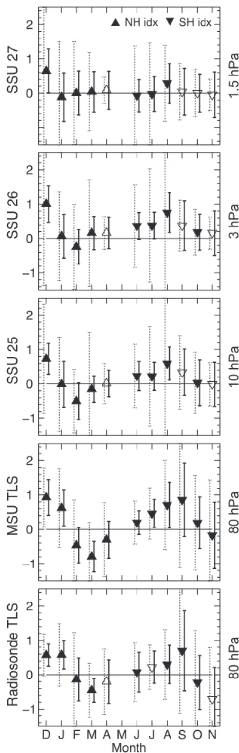
Figure 4 shows the trends in the BDC index for the MSU and SSU data, as well as the radiosonde TLS-weighted data (the latter for comparison with the MSU TLS results). Filled triangle symbols indicate that a sig-nificant out-of-phase relationship persists at all levels between the NH extratropics and tropics from December to March and between the SH extratropics and tropics from June to August (except for July in the radiosonde data), as well as October. Significance for other months varies by level. As with the zonal mean temperature trends in Fig. 1, there is good agreement between the BDC index trends calculated from the MSU TLS data and those from the TLS-weighted radiosonde data (r 5 0.86).
Uncertainties in the raw BDC index trend (dotted error bars) overwhelmingly indicate that those trends are not significant at the 2s level, with the MSU TLS December increasing trend being the only value to pass this significance test (i.e., as shown in Fig. 3). However, several trends in the adjusted BDC index are significant at the 2s level. Most strikingly, the increasing trend in the December adjusted BDC index is consistent and significant throughout the depth of stratosphere, in line with changes hinted at by the nonsignificant trends shown in Fig. 2b. Significant trends continue into January in both the MSU TLS and radiosonde TLS data. Additionally, also in line with Fig. 2b, there is a significant increasing trend in the adjusted BDC index during August from the MSU TLS level to the SSU-26 level (although notably not in the radiosonde TLS data). A significant decrease in the adjusted BDC index is apparent for March in the lower
FIG. 4. Linear trend in the BDC indices by month for the TLS-weighted radiosonde and the MSU and SSU data. Upward-pointing triangles indicate BDC index trends for an index constructed from NH extratropics minus tropics (December–April); downward-pointing triangles are for the SH extratropics minus the tropics (June–November). Filled triangles indicate where the (detrended) tropical and extratropical time series for that month are signifi-cantly anticorrelated (r , 20.38). Each point has two error bars. The dotted error bar indicates the 62s error for the BDC index calculated from ‘‘raw’’ temperature data, whereas the solid error bar indicates the 62s error for an adjusted BDC index, calculated after removal of BDC-like interannual variability (see text and Fig. 3).
stratosphere (MSU and radiosonde data), again consis-tent with the nonsignificant trends indicated in Fig. 2b.
Taking the results from the adjusted BDC index, it would appear that there is some evidence for a signifi-cant increase in the strength of both the NH branch of the BDC, during December and January, and the SH branch of the BDC, during August. Such a result is in agreement with FSL10, but here it is shown to extend beyond the MSU TLS level. For the NH branch, this increase extends throughout the depth of the strato-sphere, as sampled by the MSU and SSU instruments, whereas the strengthening extends to the midstrato-sphere (SSU-26 level) for the SH branch. While several modeling studies report the strongest seasonal trends in the BDC during the December–February season (Butchart and Scaife 2001; Butchart et al. 2006; Li et al. 2008; Garny et al. 2009; McLandress and Shepherd 2009), it is generally in the SH branch and linked with ozone depletion. The lack of a significant out-of-phase tropical– SH extratropical temperature relationship for that pe-riod means that such a trend would not show up in this analysis. As for austral winter (June–August) BDC trends, the modeling studies of Li et al. (2008) and McLandress and Shepherd (2009) both report that their SH down-welling trends are weaker even than during March–May. The lower-stratosphere negative trend in the adjusted BDC index, again in agreement with FSL10 and as sim-ilarly noted by Free (2011), could be interpreted as con-sistent with a slowdown in the BDC. However, it should be noted that apparent changes in BDC strength derived from monthly trends might represent a shift in the annual cycle of the circulation (particularly for the NH lower-stratosphere December warming/March cooling trend pattern), rather than an overall strengthening or weak-ening for a given season. This is an inherent limitation in this approach.
A more detailed analysis of the seasonal cycle in tem-peratures is beyond the scope of this particular study, but an idea of changes in the seasonal cycle can be de-termined by examining climatological annual cycles for different time periods. As suggested by Yulaeva et al. (1994), and subsequently examined in greater detail by Rosenlof (1995), the annual cycle in tropical lower-stratospheric temperatures appears to be connected to the annual cycle in NH wave activity. Figure 5a, there-fore, shows the time series of tropical average (208S– 208N) MSU TLS temperature anomalies. While there is an overall cooling trend in the tropical temperatures, the time series can also be considered to consist of a warmer period prior to 1992 and a cooler period from 1995 (see the straight lines in Fig. 5a). Based on this, Fig. 5b shows the climatological annual cycles averaged 1979–91 in-clusive and 1995–2005 inin-clusive, avoiding the period
most impacted by the eruption of Mt. Pinatubo (e.g., McCormick et al. 1995). The month of minimum tem-perature, presumably indicating the time of maximum tropical upwelling, does appear to have shifted from February in the early period to January in the later pe-riod. The timing of the maximum temperatures is still in July–August for both periods. There is also a ;0.5 K reduction in the peak-to-peak amplitude in the later period, and a 0.6-K annual average cooling.
Finally, while the trends in the adjusted BDC index are consistent with apparent shifts in the strength of the BDC, it should be cautioned that the ;30-yr time series is too short to rule out decadal variability as a driver of the observed significant BDC trends over 1979–2005. As illustrated by the apparent shift in tropical temperatures in Fig. 5a, geophysical series are often not well charac-terized by linear changes. Indeed, Fig. 6 shows the time series of the MSU TLS (NH) BDC index for March, which suggests a cooling trend persisting to the mid-1990s, followed by an increasing trend thereafter (es-pecially the 5-yr running average). A similar result was shown by Free (2011), who noted that the difference between the December and March lower-stratosphere trends in radiosonde data has been decreasing in recent
FIG. 5. Analysis of MSU TLS tropically averaged (208S–208N) temperatures. (a) Time series of temperature anomalies (thin line) and average anomalies for 1979–91 and 1995–2005 (thick lines). (b) Climatological annual temperature cycles for 1979–91 (dashed line, open circles) and 1995–2005 (solid line, filled circles).
years. Other studies have pointed to evidence for a weak-ening of the strength of the NH branch of the BDC in the 1990s, such as the persistence of the cold vortex well into spring (Waugh et al. 1999), leading to low springtime ozone values over the Arctic (e.g., Newman et al. 1997), and the apparent decrease in wave driving (e.g., Pawson and Naujokat 1999; Waugh et al. 1999; Newman and Nash 2000; Randel et al. 2002a).
5. Conclusions
Temperature trends were obtained over 1979–2005 from MSU and SSU data, and TLS-weighted radiosonde data. The trends revealed variations by season and cou-pled differences between the tropics and extratropics, although higher-latitude winter/spring trends were gen-erally not significant except at the SSU-27 level. It was demonstrated that radiosonde TLS and 30-hPa data show remarkably similar zonal mean trend patterns to the satellite data, giving further credence to their spatial and temporal patterns. When expressed relative to the global mean trend, the annual cycle in tropical and extra-tropical trends were consistent with BDC changes, with months of tropical cooling (warming) anomalies paired with extratropical warming (cooling) anomalies. How-ever, these trends were not statistically robust.
To better probe potential long-term changes in the circulation, a BDC index was constructed, based on winter/spring hemisphere extratropical temperatures minus tropical temperatures. As well as constructing the BDC index from the raw temperature data, an ad-justed index was constructed, which had BDC-like year-to-year variability subtracted, and whose trends generally had much improved statistical significance. Trends in the raw index were consistent only with a significant strengthening of the lower-stratosphere NH BDC branch in December (MSU TLS). Trends in the adjusted index
were consistent with a significant increase in the NH BDC branch in December throughout the depth of the stratosphere, with the positive trend extending into January at the lower levels (both MSU TLS and radio-sonde TLS). The adjusted index trends also suggest a significant strengthening of the SH branch of the BDC during August, from the MSU TLS level (though not radiosonde TLS) to the midstratosphere SSU-26 level. In the lower stratosphere, for the NH BDC branch, the trends in the adjusted index were consistent with a sig-nificant weakening of the BDC during March. However, this trend, paired with the apparent BDC strengthening in December–January, could just point to a change in the seasonal cycle of the circulation, that is, the timing of the peak wave driving. An examination of the differ-ences between a 1979–91 average and 1995–2005 aver-age tropical temperature seasonal cycle in the MSU TLS data revealed an apparent shift in the temperature min-imum from February to January, possibly indicative of a change in the timing of the maximum wave driving. Furthermore, the overall negative BDC index trend in March may be reflecting decadal variability, as a time series of the index is consistent with a BDC strength-ening in the last few years.
This study has attempted to diagnose BDC changes by using an empirical index based on the tropical– extratropical out-of-phase patterns apparent in the tem-perature data. Both Lin et al. (2009) and FSL10 showed significant trends in the BDC from a combination of lower-stratosphere temperature data and reanalysis in-dices of BDC strength. Trends in the BDC have also been inferred from observations by comparing the meridional structure of column ozone and lower-stratosphere tem-perature trends (Thompson and Solomon 2009). The re-sults of this present study reveal that, when working with temperature data alone, similar significant trends only be-come apparent if some effort is made to reduce year-to-year variability. Of course, temperatures are by no means an ideal measure of the BDC as many processes other than circulation affect them. In particular, temperatures in the upper stratosphere are under stronger radiative control, which makes diagnosing a dynamical signal difficult, and strong gradients in radiative trends (e.g., the ozone hole) confound the temperature-based BDC index. Furthermore, longer observational records are preferable to make a more statistically robust estimate of the BDC change, establishing the role of any decadal-scale variation in shaping longer-term trends. However, interannual variations in tempera-ture data provide a compelling signal of the BDC, and temperature observations represent our only continuous long-term observational record that could potentially shed light on any circulation changes—at the seasonal time scale and throughout the stratosphere—over the last few decades.
FIG. 6. Series of the NH BDC index for March for the MSU TLS data, constructed as in Fig. 3c. The black solid line is the raw BDC index, the black dashed line the linear trend, the thin gray line the adjusted BDC index, and the thick gray line is a 5-yr running mean of the thin gray line. Uncertainty values on the trend (for black and gray lines) correspond to 2s.
Acknowledgments. David Thompson is thanked for several contributions and comments throughout the work. Remote Sensing Systems are thanked for the provision of MSU data, sponsored by the NOAA/Climate and Global Change Program. Data are available online at http://www.remss.com. Craig Long and Roger Lin at NOAA/CDC, Bill Randel and Fei Wu at NCAR, and John Nash at the Met Office are all thanked for the pro-vision of, and information pertaining to, the SSU data. We also thank two anonymous reviewers whose com-ments greatly improved the content and clarity of this manuscript. The National Center for Atmospheric Re-search is operated by the University Corporation for At-mospheric Research under sponsorship of the National Science Foundation.
APPENDIX
Calculation of Adjusted BDC Index
For the calculation of the adjusted BDC index, it is assumed that the tropical and extratropical average temperatures can be modeled as
T1 5a1BDC 1 b1GHG1 1residuals1, (A1) T2 5a2BDC 1 b2GHG2 1residuals2, (A2) where tropical (subscript ‘‘1’’) and extratropical (subscript ‘‘2’’) temperatures T are a function of some index of BDC variability and radiative heating by greenhouse gases (GHG), with regression coefficients a and b, with residual noise remaining. If we assume that GHG is a linear function of time, we can express the detrended temperatures T9 as
T91 5a1(BDC 2 st) 1 residuals1, (A3) T92 5a2(BDC 2 st) 1 residuals2, (A4) where s is the linear trend in BDC (i.e., what we are con-cerned with) and t is time. Based on the strong interannual coupling of tropical and extratropical temperature anom-alies, adjusted tropical and extratropical temperatures T* are calculated by
T1* 5 T1 2r1T92, (A5) T2* 5 T2 2r2T91, (A6) where r1and r2are the regression coefficients from
T91 5c1 1r1T92, (A7) T92 5c2 1r2T91; (A8)
that is, the r coefficients describe the nontrend relation-ship between the tropical and extratropical temperatures. For not too high noise, (2)r1# (2)a1/a2 and (2)r2 # (2)a2/a1. Assuming that the r coefficients are exactly equal to the ratio of the a coefficients, substituting into (A5) and (A6) we have
T1* 5 a1st 1 b1GHG1 1residuals12r1residuals2, (A9) T2* 5 a2st 1 b2GHG2 1residuals22r2residuals1.
(A10) The result is the removal of the nontrend variability due to the BDC, but at the expense of increasing the residual noise (if uncorrelated between tropical and extratropical latitudes). From the differences between the two error bars in Fig. 4, we can see that removing the BDC gen-erally outweighs any increase in noise, except for some SH spring trends in the SSU data.
REFERENCES
Butchart, N., and A. A. Scaife, 2001: Removal of chlorofluoro-carbons by increased mass exchange between the stratosphere and troposphere in a changing climate. Nature, 410, 799–802. ——, and Coauthors, 2006: Simulations of anthropogenic change in the strength of the Brewer-Dobson circulation. Climate Dyn., 27, 727–741.
——, and Coauthors, 2010: Chemistry–climate model simulations of twenty-first century stratospheric climate and circulation changes. J. Climate, 23, 5349–5374.
Christy, J. R., R. W. Spencer, W. B. Norris, W. D. Braswell, and D. E. Parker, 2003: Error estimates of version 5.0 of MSU– AMSU bulk atmospheric temperatures. J. Atmos. Oceanic Technol., 20, 613–629.
Cook, P. A., and H. K. Roscoe, 2009: Variability and trends in stratospheric NO2in Antarctic summer, and implications for
stratospheric NOy. Atmos. Chem. Phys., 9, 3601–3612.
Dunkerton, T., 1978: On the mean meridional mass motions of the stratosphere and mesosphere. J. Atmos. Sci., 35, 2325–2333. Eichelberger, S. J., and D. L. Hartmann, 2005: Changes in the
strength of the Brewer-Dobson circulation in a simple AGCM. Geophys. Res. Lett., 32, L15807, doi:10.1029/2005GL022924. Engel, A., and Coauthors, 2009: Age of stratospheric air
un-changed within uncertainties over the past 30 years. Nat. Geosci., 2, 28–31.
Fels, S. B., 1985: Radiative-dynamical interactions in the middle atmosphere. Advances in Geophysics, Vol. 28A, Academic Press, 277–300.
Free, M., 2011: The seasonal structure of temperature trends in the lower tropical stratosphere. J. Climate, 24, 856–866. Fritz, S., and S. D. Soules, 1972: Planetary variations of
strato-spheric temperatures. Mon. Wea. Rev., 100, 582–589. Fu, Q., S. Solomon, and P. Lin, 2010: On the seasonal dependence
of tropical lower stratospheric temperature trends. Atmos. Chem. Phys., 10, 2643–2653.
Fueglistaler, S., A. E. Dessler, T. J. Dunkerton, I. Folkins, Q. Fu, and P. W. Mote, 2009: Tropical tropopause layer. Rev. Geo-phys., 47, RG1004, doi:10.1029/2008RG000267.
Garcia, R. R., and W. J. Randel, 2008: Acceleration of the Brewer– Dobson circulation due to increases in greenhouse gases. J. Atmos. Sci., 65, 2731–2739.
Garny, H., G. E. Bodeker, and M. Dameris, 2007: Trends and variability in stratospheric mixing: 1979-2005. Atmos. Chem. Phys., 7, 5611–5624.
——, M. Dameris, and A. Stenke, 2009: Impact of prescribed SSTs on climatologies and long-term trends in CCM simulations. Atmos. Chem. Phys., 9, 6017–6031.
Haynes, P. H., C. J. Marks, M. E. McIntyre, T. G. Shepherd, and K. P. Shine, 1991: On the ‘‘downward control’’ of extratropical diabatic circulations by eddy-induced mean zonal forces. J. Atmos. Sci., 48, 651–678.
Hegglin, M. I., and T. G. Shepherd, 2009: Large climate-induced changes in ultraviolet index and stratosphere-to-troposphere flux. Nat. Geosci., 2, 687–691.
Holton, J. R., P. H. Haynes, M. E. McIntyre, A. R. Douglass, R. B. Rood, and L. Pfister, 1995: Stratosphere-troposphere exchange. Rev. Geophys., 33, 403–439.
Hu, Y., and Q. Fu, 2009: Stratospheric warming in southern hemisphere high latitudes since 1979. Atmos. Chem. Phys., 9, 4329–4340. Lamarque, J.-F., and S. Solomon, 2010: Impact of changes in
cli-mate and halocarbons on recent lower stratosphere ozone and temperature trends. J. Climate, 23, 2599–2611.
Li, F., J. Austin, and J. Wilson, 2008: The strength of the Brewer– Dobson circulation in a changing climate: Coupled chemistry– climate model simulations. J. Climate, 21, 40–57.
Lin, P., Q. Fu, S. Solomon, and J. M. Wallace, 2009: Temperature trend patterns in Southern Hemisphere high latitudes: Novel indicators of stratospheric changes. J. Climate, 22, 6325–6341. McCormick, M. P., L. W. Thomason, and C. R. Trepte, 1995: Atmo-spheric effects of the Mt. Pinatubo eruption. Nature, 373, 399–404. McLandress, C., and T. G. Shepherd, 2009: Simulated anthropo-genic changes in the Brewer–Dobson circulation, including its extension to high latitudes. J. Climate, 22, 1516–1540. Mears, C., and F. J. Wentz, 2009: Construction of the Remote
Sensing Systems v3.2 atmospheric temperature records from the MSU and AMSU microwave sounders. J. Atmos. Oceanic Technol., 26, 1040–1056.
Newman, P. A., and E. R. Nash, 2000: Quantifying the wave driving of the stratosphere. J. Geophys. Res., 105, 12 485–12 497. ——, J. F. Gleason, R. D. McPeters, and R. S. Stolarski, 1997:
Anom-alously low ozone over the Arctic. Geophys. Res. Lett., 24, 2689– 2692.
Olsen, M. A., M. R. Schoeberl, and J. E. Nielsen, 2007: Response of stratospheric circulation and stratosphere-troposphere ex-change to changing sea surface temperatures. J. Geophys. Res., 112, D16104, doi:10.1029/2006JD008012.
Pawson, S., and B. Naujokat, 1999: The cold winters of the middle 1990s in the northern lower stratosphere. J. Geophys. Res., 104, 14 209–14 222.
Ramaswamy, V., and Coauthors, 2001: Stratospheric temperature trends: Observations and model simulations. Rev. Geophys., 39, 71–122.
Randel, W. J., and F. Wu, 1999: Cooling of the Arctic and Antarctic polar stratospheres due to ozone depletion. J. Climate, 12, 1467– 1479.
——, R. R. Garcia, and F. Wu, 2002a: Time-dependent upwelling in the tropical lower stratosphere estimated from the zonal mean momentum budget. J. Atmos. Sci., 59, 2141–2152. ——, F. Wu, and R. S. Stolarski, 2002b: Changes in column ozone
correlated with the stratospheric EP flux. J. Meteor. Soc. Japan, 80, 849–862.
——, ——, H. Vo¨mel, G. Nedoluha, and P. M. D. Forster, 2006: De-creases in stratospheric water vapor after 2001: Links to changes in the tropical tropopause and the Brewer-Dobson circulation. J. Geophys. Res., 111, D12312, doi:10.1029/2005JD006744. ——, and Coauthors, 2009: An update of observed stratospheric temperature trends. J. Geophys. Res., 114, D02107, doi:10.1029/ 2008JD010421.
Ray, E. A., and Coauthors, 2010: Evidence for changes in strato-spheric transport and mixing over the past three decades based on multiple datasets and tropical leaky pipe analysis. J. Geo-phys. Res., 115, D21304, doi:10.1029/2010JD014206. Rosenlof, K. H., 1995: Seasonal cycle of the residual mean
me-ridional circulation in the stratosphere. J. Geophys. Res., 100, 5173–5191.
——, and R. C. Reid, 2008: Trends in the temperature and water vapor content of the tropical lower stratosphere: Sea surface connection. J. Geophys. Res., 113, D06107, doi:10.1029/ 2007JD009109.
Santer, B. D., T. M. L. Wigley, J. S. Boyle, D. J. Gaffen, J. J. Hnilo, D. Nychka, D. E. Parker, and K. E. Taylor, 2000: Statistical significance of trends and trend differences in layer-average atmospheric temperature time series. J. Geophys. Res., 105, 7337–7356.
Sherwood, S. C., 2007: Simultaneous detection of climate change and observing biases in a network with incomplete sampling. J. Climate, 20, 4047–4062.
——, C. L. Meyer, R. J. Allen, and H. A. Titchner, 2008: Robust tropospheric warming revealed by iteratively homogenized radiosonde data. J. Climate, 21, 5336–5352.
Shine, K. P., 1987: The middle atmosphere in the absence of dy-namical heat fluxes. Quart. J. Roy. Meteor. Soc., 113, 603–633. ——, and Coauthors, 2003: A comparison of model-simulated trends in stratospheric temperatures. Quart. J. Roy. Meteor. Soc., 129, 1565–1588.
——, J. J. Barnett, and W. J. Randel, 2008: Temperature trends derived from stratospheric sounding unit radiances: The effect of increasing CO2on the weighting function. Geophys. Res.
Lett., 35, L02710, doi:10.1029/2007GL032218.
Solomon, S., 1999: Stratospheric ozone depletion: A review of concepts and history. Rev. Geophys., 37, 275–316.
Sudo, K., M. Takahashi, and H. Akimoto, 2003: Future changes in stratosphere-troposphere exchange and their impacts on fu-ture tropospheric ozone simulations. Geophys. Res. Lett., 30, 2256, doi:10.1029/2003GL018526.
Thompson, D. W. J., and S. Solomon, 2005: Recent stratospheric climate trends as evidenced in radiosonde data: Global structure and tropospheric linkages. J. Climate, 18, 4785–4795. ——, and ——, 2009: Understanding recent stratospheric climate
change. J. Climate, 22, 1934–1943.
Ueyama, R., and J. M. Wallace, 2010: To what extent does high latitude wave forcing drive tropical upwelling and the Brewer– Dobson circulation? J. Atmos. Sci., 67, 1232–1246.
Waugh, D. W., R. J. Randel, S. Pawson, P. A. Newman, and E. R. Nash, 1999: Persistence of the lower stratospheric polar vor-tices. J. Geophys. Res., 104, 27 191–27 201.
Young, P. J., D. W. J. Thompson, K. H. Rosenlof, S. Solomon, and J.-F. Lamarque, 2011: The seasonal cycle and interannual variability in stratospheric temperatures and links to the Brewer–Dobson circulation: An analysis of MSU and SSU data. J. Climate, 24, 6243–6258.
Yulaeva, E., J. R. Holton, and J. M. Wallace, 1994: On the cause of the annual cycle in tropical lower-stratospheric temperatures. J. Atmos. Sci., 51, 169–174.