HAL Id: hal-01308433
https://hal.archives-ouvertes.fr/hal-01308433
Submitted on 27 Apr 2016
HAL is a multi-disciplinary open access archive for the deposit and dissemination of sci-entific research documents, whether they are pub-lished or not. The documents may come from teaching and research institutions in France or abroad, or from public or private research centers.
L’archive ouverte pluridisciplinaire HAL, est destinée au dépôt et à la diffusion de documents scientifiques de niveau recherche, publiés ou non, émanant des établissements d’enseignement et de recherche français ou étrangers, des laboratoires publics ou privés.
Distributed under a Creative Commons Attribution - NonCommercial - NoDerivatives| 4.0 International License
Optimal Energy Management Using Model Predictive
Control: Application to an Experimental Building
Nils Artiges, Alexandre Nassiopoulos, Franck Vial, Benoit Delinchant
To cite this version:
Nils Artiges, Alexandre Nassiopoulos, Franck Vial, Benoit Delinchant. Optimal Energy Management Using Model Predictive Control: Application to an Experimental Building. Climamed 2015 - Mediter-ranean congress of HVAC, Sep 2015, Juan-les-pins, France. �hal-01308433�
Optimal Energy Management Using Model Predictive Control : Application to an
Experimental Building
Nils ARTIGES1,2, Alexandre NASSIOPOULOS1, Franck VIAL2, Benoit DELINCHANT3
1LUNAM University, IFSTTAR, CoSys, 44344 Bouguenais, France
2Univ. Grenoble Alps, CEA, LETI, MINATEC Campus, F-38054 Grenoble, France 3Univ. Grenoble Alps, G2ELab, F-38000 Grenoble, France
[email protected], [email protected]
[email protected], [email protected]
SUMMARY
In energy-efficient buildings, the interactions and coupling effects between the building, its environment and its conditions of use play an important role on the energy balance. Recent development in information and communication technologies enable to have real time information about current and future environ-mental conditions, energy price or CO2 concentrations. Thus, it becomes possible to design building man-agement systems that exploit these data in real time in order to optimize occupants comfort and energy performance. Model predictive control relies on a numerical model and real time measurements to com-pute an optimal strategy. This paper shows an example of application on a experimental building where both heating and ventilation are simultaneously controlled. Model predictive control is here computed so as to minimize a criterion based on operative temperature and energy consumption. The computation uses data collected on-site by temperature and power sensors, as well as weather data collected online through web-services. We describe here the deployment phase which includes a model calibration process in order to ensure optimality of the results. Both model calibration and optimal management are computed using a multizone thermal model. During optimization phases, the adjoint method is employed to derive effi-ciently descent algorithms. These choices make the whole software part of the system flexible and fast enough to be embedded on-board on a domestic building management system.
INTRODUCTION
Usual control strategies used in buildings rely on well-established regulation algorithms (Proportional-Integral-Derivative (PID) controllers for example). A PID controller aims at commanding one or several system inputs (i.e. heaters power) to make an output variable (i.e. room temperature) match a desired set-point. Methods of this kind are designed to achieve a defined thermal comfort, but due to their formula-tion, they are not adapted to take into account some energy criteria, nor to anticipate future variations of usage and weather conditions.
In Model Predictive Control (MPC), the control problem is formulated like an optimization problem [1, 2]. This point enables high performance thermal management in buildings since power reduction goals can be formulated directly in the control process, providing anticipation of energetic gains [3, 4, 5] and thermal state predictions. Simulation studies promise around 20% of consumption reduction [6]. More-over, recent developments in embedded informatics, (wireless) sensor networks, communication protocols dedicated to buildings applications (LonWorks, KNX, Zigbee...) strongly increases the deployability po-tential of such methods in all kind of buildings.
A model predictive control relies on :
• A model describing all the dynamics of the controlled process
• Predictions of model inputs, to perform command optimization over future times • Online estimations (of states, parameters) to correct model errors during operation
Since a MPC strategy is model-based, the control quality depends on the model quality. Identification techniques are used to calibrate uncertain model parameters.
In this work, we present an optimal predictive control method designed for buildings thermal and ener-getic management, applied on the case of INCAS I-MA, an instrumented domestic house. We firstly de-scribe the INCAS house and formalisms used for its modelization. Then we dede-scribe the whole control process and the adjoint method used to solve efficiently all optimization sub-processes. Then we present and discuss obtained results in a one month on-site experimentation.
INCAS I-MA DESCRIPTION AND MODELIZATION
Building description
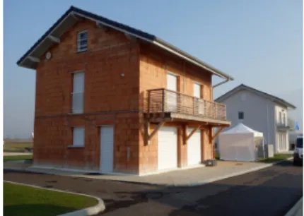
The INCAS I-MA house is an experimental building of the INES institute, located at Savoie Technolac, Chambéry, France. This building is designed like a classic two-floors domestic dwelling, built with mod-ern construction materials and techniques.
Figure 1: INCAS I-MA building before aerogel coating
Walls are made of brick blocks with an outside aerogel plaster, and a standard gypsum cover inside. This building is provided with numerous temperature sensors : at each material interface within the walls, at the inner and outer surface of the walls and inside each room. A solar sensor provides diffuse and direct solar radiation. Each room has an electric heater and is connected to a centralized CMV (Controlled Me-chanical Ventilation) system.
Numerical implementation
For our research work, our team developed ReTrofiT, a Matlab code toolbox dedicated to building model-ing, simulation and optimization [7]. The main advantage of the ReTrofiT approach lies in the use of this built-in optimization tool adapted to real-time applications.
Models used by ReTrofiT are built on standard multizone assumptions for temperatures and heat flows [8], and the application of the heat equation. The main assumptions are homogenous temperature and pressure for each thermal zone, and one-directional thermal conduction through multi-layered walls. We also added low order HVAC models (electric heater and CMV), and a CO2 concentration model. The
model structure of each building is built from a gbXML model file, generated by a CAD software. Then the continuous model is discretised with first order finite elements within walls, and an Euler implicit scheme in time.
ReTrofiT also provides an efficient optimization algorithm based on the adjoint theory [9]. An adjoint model is generated from the direct model and quadratic cost function over temperatures and model pa-rameters. The adjoint theory shows that cost function gradients can be expressed directly as functions of direct and adjoint model solutions, that is far more efficient than with a finite differences scheme. The computed gradient is then directly used in gradient descent techniques.
AN OPTIMAL PREDICTIVE CONTROL PROCESS
Optimal control
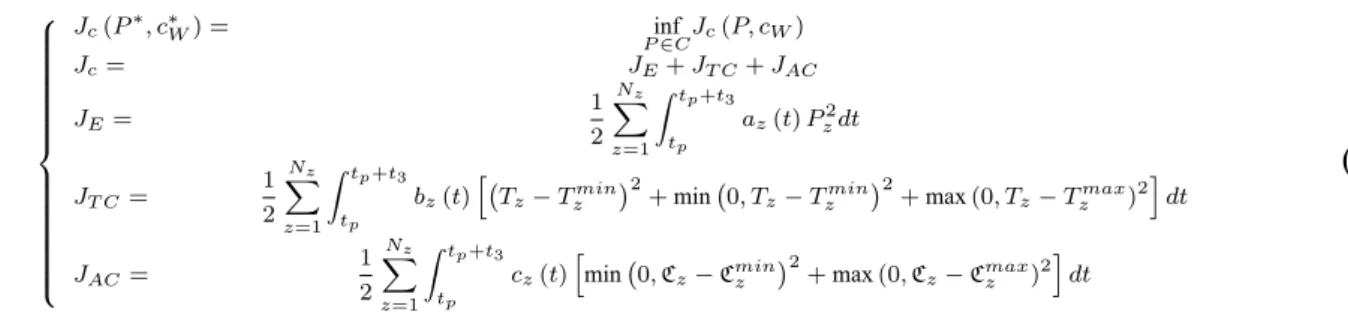
Compared with a PID control (Porportional Integral Derivative), an optimal control can handle other ob-jectives than a simple setpoint, such energy consumption or constraints violation, taking in account dy-namic effects (passive thermal storage in walls for instance). In our case, we compute the optimal com-mand set (P∗, c∗w), where P is the electrical power injected in heaters and cw is the CMV air flow, such
that : Jc(P∗, c∗W) = Pinf∈CJc(P, cW) Jc= JE+ JT C+ JAC JE= 1 2 Nz ∑ z=1 ˆtp+t3 tp az(t) Pz2dt JT C= 1 2 Nz ∑ z=1 ˆtp+t3 tp bz(t) [( Tz− Tzmin )2 + min(0, Tz− Tzmin )2 + max (0, Tz− Tzmax)2 ] dt JAC= 1 2 Nz ∑ z=1 ˆtp+t3 tp cz(t) [ min(0, Cz− Cminz )2 + max (0, Cz− Cmaxz )2 ] dt (1)
JE is a quadratic cost term related to the instantaneous electrical power consumption. JT C is a thermal
comfort cost that penalizes the temperature difference with a minimum temperature setpoint Tmin and every temperature value outside temperature bounds Tminand Tmax. JACis an air quality term that
penal-izes CO2 concentrations C outside sanitary bounds Cminz and C max z .
az, bzand cz are time-dependent weights used to manage a tradeoff between these different cost terms.
They are also used for normalization (to provide JE, JT C and JACwith similar orders of magnitude) and
to take into account building occupancy : if nobody is present in room z at instant t, then bz(t) and cz(t)
must be equal to 0.
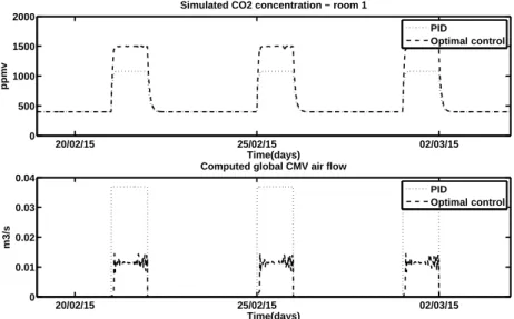
We can easily see the differences between an optimal control and a PID control in simulation. We simu-lated a PID control with a PID controller for each heater, tuned for a 20°C setpoint, and shut off during absences. For the PID strategy, the CMV airflow is maximal during presence and shut off during absence. For the optimal command, we set the same temperature setpoint for JT C (but no temperature constraints
for this simulation case), and a CO2maximal constraint of 1500 ppmv. With a, b, and c coefficients
prop-erly tuned, we get an optimal control (2,3) with an incomfort cost JT C+ JAC and a total electric
consump-tion (heaters and CMV motor) respectively 9.5% and 0.12% lower than with the PID control.
20/02/15 25/02/15 02/03/15 10 15 20 Time(days) C
Simulated temperatures − room 1
PID Optimal control Setpoint 20/02/15 25/02/15 02/03/15 0 200 400 600 800 1000 1200 Time(days) W
Computed Electrical Power − Heater room 1
PID
Optimal control
20/02/15 25/02/15 02/03/15 0 500 1000 1500 2000 Time(days) ppmv
Simulated CO2 concentration − room 1
PID Optimal control 20/02/15 25/02/15 02/03/15 0 0.01 0.02 0.03 0.04 Time(days) m3/s
Computed global CMV air flow
PID
Optimal control
Figure 3: Optimal control vs. PID control : CO2 (ppmv) and CMV air flow
(
m3/s)
With the optimal control, we have visible effects of anticipation with a preheat before occupancy periods, and automatic CMV management compliant with CO2maximal concentration. The optimal command
smooth temperature variations during occupancy, but can allow a distance with the setpoint if bz is not
high.
However, such optimal command cannot be implemented directly, due to model errors and initial state errors : it needs to be implemented in a global process (described in the following section) including a calibration step (to correct model errors) and an estimation step (to give a good guess of the initial state). It is also important to point out that such quadratic formulation has useful mathematical properties for optimization problem solving, but the quadratic norm on the electrical power doesn’t represent the true consumed power. We use it there for the sake of simplicity, since it doesn’t change our methodology, but a practical implementation should consider the true consumed power. In this case, the consideration of temperature boundaries and a quadratic cost on the difference with the minimal temperature helped the consumption reduction.
Global process
We present herein an optimal predictive control process that aims at optimize the global energy consump-tion and the thermal comfort of a building. The global process is divided in several tasks performed se-quentially.
The calibration step is performed once to recover good model parameters values and ensures that the model behavior matches reality. An estimation step is then performed just before a command computa-tion to compensate model deviacomputa-tions over time (this adds some online error correccomputa-tion to the global pro-cess) and give a good initialization for command computation. Both estimation and command steps are repeated periodically over time. Calibration, estimation and command computation consist in different optimization tasks : in each case, a quadratic cost function defining the optimization problem has to be minimized.
Model calibration
The calibration consists in determining values of uncertain parameters (like convective heat transfer coef-ficients) that minimize the distance between measured and simulated temperatures. This task is commonly found in literature as an inverse problem. Such problem is treated extensively in [10]. Previous work of our team focused on identification problems applied on buildings for monitoring and diagnosis purposes [11, 12, 13, 14]. In our case, we formulated the identification problem by the following optimization prob-lem : Ji(p) = inf p∈UJi(p) Ji = 1 2 Ni Σ i=1 ˆ ti 0 (T (t)− Tmi(t)) 2 dt (2)
Were p is the vector of unknown parameters, Tmthe vector of temperature measurements (Ni sensors) and T the corresponding vector of simulated temperatures.
Due to its ill-posedness nature, this problem is quite hard to solve and some factors have a direct impact on its solvability :
• Integration time support [0, ti] : If too short, identification may not converge, or converge towards
false values. In this case, almost several days is mandatory.
• Identified parameters p : For a given observation Tm, all the unknown parameters may not be
iden-tified. Some of them may not have a significant influence on measured temperatures and several pa-rameters could have a very similar effect. They must be chosen among several identification tests, with the help of the physical knowledge of the building.
• Temperature measurements Tm: The more sensors are used, the more precise the identification.
However, any bias in measurements may have an important impact.
• Initial conditions : The initial temperature field must be the closest to reality, otherwise it will per-turb the identification quality. An initial condition error can be absorbed by a long integration time support. One can also use interpolation on measured temperatures to provide an estimation of the temperatures field.
The quality of the calibration step is evaluated here in terms of predicatbility. Indeed, we only want to have good simulations results for any solicitations, and not only for a single meteorological scenario.
Estimation
Even well calibrated, the error of the simulated model response increases over time. Besides, as explained in the next section, an optimal command computation needs an accurate estimation of the initial state of the building, and real time measurements Tm provide only a subset of the full field of temperatures. The
estimation step aims at periodically computing a corrective parameter to correct this drift. As the response of the corrected model is better, its simulation provides a good estimation T∗ of the full thermal state at time tp, used as initial conditions for the command step. This estimation step is formulated like the
T∗ = T (tp,Q∗) Je(Q∗) = inf Q∈UJe(Q) Je= 1 2 Nz Σ z=1 ˆ tp tp−t2 (Tz(Q) − Tmz)2dt (3)
In this case, we compute the internal gainsQ∗(t) that minimize the error between simulated and measured room temperatures. These parameters influence directly zone temperatures that are directly involved in the comfort term used in the control step. Initial conditions T (tp − t2) for the estimation phase are
pro-vided by interpolation over measurements. The time (tp− t2) must be long enough to reduce the impact of
initialization errors (several hours).
Control synthesis
The control synthesis consists here in solving the problem (1). One main difference with the other opti-mization tasks lies in the predictive nature of our problem. Since the integration time support [tp,tp+ t3]
takes place in the future, meteorological and occupancy inputs used in our model are forecasts provided by occupancy scenarios and meteorological services. The previous estimation step gives an initial state for the optimal command computation.
EXPERIMENTAL RESULTS
For our experimental tests, we have chosen to implement an optimal control of two rooms which controls their heaters and the CMV airflow. Firstly, we performed the offline calibration task with measurements recovered from previous experimentation. Then, estimation and control tasks were computed on a distant server recovering measurements from the house and sending commands in real time during one month. Both estimation and control tasks were repeated sequentially with a 3-hour time-step, estimation time t2
was set to 48 hours and prediction time t3to 24 hours.
Calibration
At the calibration stage, for technical reasons, we had only access to three temperature measurements over a six-day and a three-day period : two ambient room temperatures and the inner surface temperature of an external wall of the first room. The following parameters were identified : walls thermal conductivities and capacities, convection exchange coefficients, percentages of CMV total airflow per room, windows radiative transmittance and surfaces absorbances.
The calibrated model response gives quite good results for the meteorological dataset used for calibration (figure 5 right). However, After convergence, some parameters have converged towards 0 and prediction error was still quite high, but better than before calibration. To deal with divergence due to calibration errors, we set a three hour update time for estimation and command steps to handle reasonable prediction errors.
Figure 5: Calibration results
Estimation
For the estimation task, we have only used room temperature measurements. Left figures 6 represent a single step result, and right figures result of repeated estimation steps.
Figure 6: Estimation and prediction results
Computed internal gains are greater at initial times because of initialization errors, but this correction leads to a very good fit between measured and simulated temperatures (figure 6 left). For predictions, we use the last computed internal gains value as a constant correction. Since the model is not perfectly cal-ibrated, we observe an important variation of this corrective value among estimation steps (figure 6 top-right), but this strategy leads to a good performance for temperature predictions, with a standard deviation of 0.8 °C for errors between estimation steps (figure 6 bottom-right).
Command
We applied in the real case the same optimal command problem presented in simulation, but with addi-tional temperature bounds. The main difficulty in command synthesis is the tuning of weight coefficients. Indeed, the related optimization problem is a multi-objective problem formulated like a mono-objective problem by the use of these time-dependent coefficients. We performed some preliminary tests (simula-tions) to determine a convenient tuning such that each objective has a sufficient impact over computed control. Effects of anticipation are visible in figure 7 : highest power peaks are observed just before oc-cupancy periods (rise of temperature lower bound). Meanwhile, we observed a CMV air flow reduction
during absences. Discontinuities in the command law are a consequence of the sequential evaluation of corrective internal gains. A better calibrated model would lead to a smoother command.
Figure 7: Optimal command results
CONCLUSIONS AND PERSPECTIVES
This paper presents an optimal predictive control strategy for buildings based on a multizone model and an adjoint based optimizer for efficient real-time implementations. Application results on an experimental building show anticipation effects and a good respect of temperature constraints.
Further tests will involve a better calibrated model, with more available sensors and a longer time period. Next studies will focus on developing methods for an easier deployment in buildings. Indeed, the choice of the model, the number and type of sensors, as well as the tuning process are time consuming and need an expert level for each individual implementation, which is not convenient for large deployments.
ACKNOWLEDGMENTS
Part of this work has been supported by French Research National Agency (ANR) through the PRECCI-SION project (ANR-12-VBDU-0006), part of Villes et Batiments Durables program. We specially thank the INES Institute (Pierre Bernaud, Adrien Brun) for their technical support and giving us access to the house, the Vesta-System company (Binh Xuan Hoa Le, Stéphane Bergeon) for the software supervision system, and Power-Lan (William Martin) for the online monitoring service.
REFERENCES
[1] David W. Clarke, C. Mohtadi, and P. S. Tuffs, “Generalized predictive control Part I. The basic algorithm”, Automatica, vol. 23, no. 2, pp. 137–148, 1987.
[2] Jan Marian Maciejowski, Predictive Control: With Constraints, Pearson Education, January 2002.
[3] Ion Hazyuk, Christian Ghiaus, and David Penhouet, “Optimal temperature control of intermittently heated buildings using Model Predictive Control: Part I Building modeling”, Building and Environment, vol. 51, pp. 379–387, 2012.
[4] Gregor P. Henze, Clemens Felsmann, and Gottfried Knabe, “Evaluation of optimal control for active and passive building thermal storage”, International Journal of Thermal Sciences, vol. 43, no. 2, pp. 173–183, 2004.
[5] Henrik Karlsson and Carl-Eric Hagentoft, “Application of model based predictive control for water-based floor heating in low energy residential buildings”, Building and Environment, vol. 46, no. 3, pp. 556–569, March 2011.
[6] Mohamed Yacine Lamoudi, Distributed model predictive control for energy management in buildings, PhD thesis, Universite de Grenoble, November 2012.
[7] Alexandre Nassiopoulos, Jordan Brouns, Nils Artiges, Mostafa Smail, and B. Azerou, “ReTrofiT: A Software to Solve Optimization and Identification Problems Applied to Building Energy Management”, 2014.
[8] Joseph Clarke, Energy Simulation in Building Design, Taylor & Francis, 2001.
[9] Jacques Louis Lions, Optimal control of systems governed by partial differential equations, Springer-Verlag, 1971. [10] Necati Ozisik and Helcio R. B. Orlande, Inverse Heat Transfer: Fundamentals and Applications, Taylor & Francis
Group, 2000.
[11] A. Nassiopoulos and F. Bourquin, “Real-time monitoring of building energy behaviour: a conceptual framework”, 2010. [12] Jordan Brouns, Alexandre Nassiopoulos, Frederic Bourquin, and Karim Limam, “State-parameter identification problems
for accurate building energy audits”, 2013.
[13] Frederic Bourquin and Alexandre Nassiopoulos, “Inverse reconstruction of initial and boundary conditions of a heat transfer problem with accurate final state”, International Journal of Heat and Mass Transfer, vol. 54, no. 15 16, pp. 3749–3760, 2011.
[14] Audrey Le Mounier, Benoit Delinchant, and Stephane Ploix, “Determination of relevant model structures for self-learning energy management system”, in Building Simulation Optimisation, June 2015.