Centuries of thermal sea-level rise due to anthropogenic emissions of short-lived greenhouse gases

Centuries of thermal sea-level rise due to anthropogenic

emissions of short-lived greenhouse gases

The MIT Faculty has made this article openly available.

Please share

how this access benefits you. Your story matters.

Citation

Zickfeld, Kirsten; Solomon, Susan andGilford, Daniel M. “Centuries

of Thermal Sea-Level Rise Due to Anthropogenic Emissions of

Short-Lived Greenhouse Gases.” Proceedings of the National

Academy of Sciences 114, no. 4 (January 2017): 657–662 © 2017

National Academy of Sciences

As Published

http://dx.doi.org/10.1073/pnas.1612066114

Publisher

National Academy of Sciences (U.S.)

Version

Final published version

Citable link

http://hdl.handle.net/1721.1/109913

Terms of Use

Article is made available in accordance with the publisher's

policy and may be subject to US copyright law. Please refer to the

publisher's site for terms of use.

Centuries of thermal sea-level rise due to

anthropogenic emissions of short-lived

greenhouse gases

Kirsten Zickfelda,1_{, Susan Solomon}b,1_{, and Daniel M. Gilford}b

a_{Department of Geography, Simon Fraser University, Burnaby, BC, Canada V5A 1S6; and}b_{Department of Earth, Atmospheric and Planetary Sciences,}

Massachusetts Institute of Technology, Cambridge, MA 02139-4307

Edited by Veerabhadran Ramanathan, Scripps Institution of Oceanography, University of California, San Diego, La Jolla, CA, and approved December 13, 2016 (received for review July 21, 2016)

Mitigation of anthropogenic greenhouse gases with short lifetimes (order of a year to decades) can contribute to limiting warming, but less attention has been paid to their impacts on longer-term sea-level rise. We show that short-lived greenhouse gases contribute to sea-level rise through thermal expansion (TSLR) over much longer time scales than their atmospheric lifetimes. For example, at least half of the TSLR due to increases in methane is expected to remain present for more than 200 y, even if anthropogenic emissions cease alto-gether, despite the 10-y atmospheric lifetime of this gas. Chlorofluo-rocarbons and hydrochlorofluoChlorofluo-rocarbons have already been phased out under the Montreal Protocol due to concerns about ozone depletion and provide an illustration of how emission reductions avoid multiple centuries of future TSLR. We examine the“world avoided” by the Montreal Protocol by showing that if these gases had instead been eliminated in 2050, additional TSLR of up to about 14 cm would be expected in the 21st century, with continuing contri-butions lasting more than 500 y. Emissions of the hydrofluorocarbon substitutes in the next half-century would also contribute to centuries of future TSLR. Consideration of the time scales of reversibility of TSLR due to short-lived substances provides insights into physical processes: sea-level rise is often assumed to follow air temperature, but this assumption holds only for TSLR when temperatures are increasing. We present a more complete formulation that is accurate even when atmospheric temperatures are stable or decreasing due to reductions in short-lived gases or net radiative forcing.

climate change

|

|

|

|

A

nitrous oxide (N2O), and halocarbons (HCs), have increased since

the beginning of the industrial revolution and have been the main drivers of warming global air and ocean temperatures as well as rising sea levels (1). The goal of this paper is to assess whether the sea-level rise through thermal expansion (TSLR) induced by an-thropogenic increases in GHGs that are short-lived (i.e., those with atmospheric residence times of years to decades) is reversible, and on what time scales (2, 3). We also discuss the TSLR due to long-lived gases (defined here as those with residence times of several centuries or longer) and show how the comparison of re-sponses of TSLR to different gases elucidates the climate-system processes that control TSLR reversibility. Understanding how emissions of different gases each affect the Earth’s climate over time is central to policy evaluation (e.g., when tradeoffs between mitigation options for different GHGs are considered).

A fundamental goal of the United Nations Framework Con-vention on Climate Change (UNFCCC) and its Paris agreement is the stabilization of GHGs at a level that would avoid dangerous anthropogenic interference with the climate system. Future emis-sion pathways that would lead to stabilized concentrations of an-thropogenic GHGs, and the attendant consequences for global warming and sea-level rise, have been examined with a wide range

of approaches, including models and semiempirical studies (1). Com-mitments to further changes in air temperatures and TSLR even after stabilization of CO2and other forcing agents have also been estimated

(1). In addition to stabilization, the“potentially irreversible threat to human societies and the planet” (ref. 4, p. 1) from climate changes is important in assessing risk, and both stabilization and irreversibility are cornerstones of the UNFCCC and Paris agreements (4).

Recent studies by many different groups have shown that the at-mospheric warming due to anthropogenic CO2emissions is expected

to remain nearly constant for more than a millennium, even if manmade emissions were to stop entirely, so that this climate change is essentially irreversible on human time scales. Whereas atmospheric temperatures remain approximately constant, the as-sociated TSLR is expected to continue to increase for centuries even after emissions cease, based on both Earth system models of intermediate complexity (EMICs) (5–9) and general circulation model (GCM)-based Earth system models (10–13). Note that in this paper, we do not evaluate hypothetical geoengineering mea-sures that may be able to remove gases from the atmosphere or induce active atmospheric cooling to counter warming. However, our results are relevant to understanding how TSLR should be expected to respond even if such measures were eventually able to safely and effectively produce net atmospheric cooling, as discussed below.

In contrast to the irreversible climate impacts of CO2

emis-sions, the atmospheric warming impact of short-lived climate pollutants can in principle be reversed on time scales of decades if anthropogenic emissions were to decrease or cease (14–16). The most abundant short-lived climate-forcing agent is CH4,

Significance

Human activities such as fossil-fuel burning have increased emissions of greenhouse gases (GHGs), which have warmed

the Earth’s atmosphere and ocean and caused sea levels to rise.

Some of these GHGs (e.g., methane) have atmospheric life-times of decades or less, whereas others (e.g., carbon dioxide) persist for centuries to millennia. As policy seeks to reduce climate changes, it is important to understand how mitigation of different gases each contributes to this goal. Our study shows that short-lived GHGs contribute to thermal expansion of the ocean over much longer time scales than their atmospheric lifetimes. Actions taken to reduce emissions of short-lived gases could mitigate centuries of additional future sea-level rise. Author contributions: K.Z. and S.S. designed research; K.Z. and D.M.G. performed re-search; K.Z. and D.M.G. analyzed data; and K.Z., S.S., and D.M.G. wrote the paper. The authors declare no conflict of interest.

This article is a PNAS Direct Submission.

1_{To whom correspondence may be addressed. Email: kzickfel@sfu.ca or solos@mit.edu.}

This article contains supporting information online atwww.pnas.org/lookup/suppl/doi:10. 1073/pnas.1612066114/-/DCSupplemental.

SU

with an atmospheric lifetime of about a decade, and it is the second largest contributor to global warming, after CO2(1).

Mitigation of CH4and other short-lived climate pollutants has

been discussed as a way to reduce the risk of exceeding 2 °C of global warming (16), and it is reasonable to suggest that these pollutants may also be considered in pursuing efforts toward a more ambitious 1.5 °C target under the Paris agreement (15). Furthermore, the potential of mitigation of short-lived pollutants to reduce future sea-level rise has been highlighted (17). Here, we show that the TSLR from short-lived climate-forcing agents is much less reversible than their corresponding atmospheric warm-ing, with effects that persist for centuries even after emissions stop. We explicitly consider the influences of CH4and HCs [including

chlorofluorocarbons (CFCs), hydrochlorofluorocarbons (HCFCs), hydrofluorocarbons (HFCs), and perfluorinated gases] if their anthropogenic emissions were to cease. Although the CFCs are longer-lived than CH4or most HFCs, they are relatively

short-lived compared with CO2. We evaluate the continuing TSLR that

is expected to occur due to the CFCs emitted to date, and we consider how much future TSLR has been avoided due to the Montreal Protocol, which has phased out production of these compounds. We use a state-of-the-art EMIC, the University of Victoria Earth System Climate Model (UVic ESCM) (Methods).

A number of studies have developed empirical relationships between sea-level rise and atmospheric warming (18, 19), but less work has examined these relationships when the atmospheric temperature is cooling or constant. Bouttes et al. (3) developed a relationship between sea-level rise and radiative forcing (RF) rather than atmospheric warming. Here, we build on the work of Bouttes et al. to develop a framework for understanding TSLR that is valid regardless of whether atmospheric temperatures are decreasing or increasing and show the framework’s value for un-derstanding relevant physics.

Results and Discussion

Dependence on GHG.Fig. 1 shows the model-calculated temper-ature and TSLR response to past and future anthropogenic emissions of CO2, CH4, N2O, and HCs. We use a high-emission

scenario (RCP8.5) to year 2050 and zero anthropogenic emissions of these gases thereafter (Methods). When emissions are set to zero, atmospheric CO2starts to decline. On decadal time scales,

the decline in atmospheric CO2 is governed by CO2 uptake by

the land carbon sink and dissolution and buffering of CO2in the

ocean mixed layer. Saturation of these sinks leads to slowing of the CO2decline after a few decades, as seen in Fig. 1A. On centennial

time scales, atmospheric CO2uptake is controlled by buffering of

CO2 in the deep ocean, whereas on millennial time scales, the

dominant process is dissolution of CaCO3 in sediments, which

restores the ocean’s buffer capacity (20). In our simulation, about 50% of the total emitted CO2remains in the atmosphere 750 y

after emissions cease. The persistence of the CO2perturbation is

dependent on the magnitude of the CO2emission, with larger CO2

perturbations persisting longer (8), and the strength of climate-carbon cycle feedbacks in the model. An EMIC intercomparison shows that in the UVic ESCM, the fraction of excess CO2

remaining in the atmosphere after 100 y is close to the model mean, whereas the fraction remaining after 1,000 y is at the upper end of the model range for emission pulses of both 100 and 5,000 gigatons of carbon (21).

Removal of N2O, CH4, and HCs from the atmosphere and the

associated decline in RF (Fig. 1B) is much faster than that for CO2. Removal of these gases is controlled by well-known chemical

reactions in the atmosphere and follows an exponential decline with a single time constant, which corresponds to the atmospheric lifetime of the gas [about a decade for CH4and 120 y for N2O

(22)]. For CO2 and CH4, the decline in RF as concentrations

decrease is delayed because the radiative effects of these gases are not optically thin, yielding a nonlinear relationship between at-mospheric concentration and RF (2). N2O and HCs, on the other

A

B

C

D

Fig. 1. Climate response computed with the UVic ESCM for a scenario with emissions of CO2, CH4, N2O, and HCs (including CFCs, HFCs, HCFCs, and

per-fluorocarbons) following RCP8.5 to year 2050 and zero anthropogenic emissions thereafter. (A) Atmospheric CO2concentration. (B) Total RF. (C) SAT anomaly

relative to year 1800. (D) Ocean thermal expansion relative to year 1800. GHGs are changed sequentially in the model simulations to isolate the contributions of each gas.

hand, are optically thin and do not display nonlinear spectral ef-fects. Lifetimes of HCs span a wide range from a year or a few decades for many HFCs and HCFCs, to 50–100 y for CFCs and tens of thousands of years for perfluorocarbons such as CF4(22).

Due to these long-lived gases, 0.02 W/m2HC RF (corresponding to 6% of the peak HC RF in RCP 8.5) persists for over 1,000 y. Fig. 1C shows that surface-air warming remains approximately constant for 1,000 y after elimination of CO2 emissions. The

warming contribution from N2O, HCs and CH4 decays more

quickly than that from CO2, but more slowly than what would be

expected based simply on the atmospheric lifetime of these gases (2). One hundred years after emissions cease, 71% of the peak warming still persists for N2O, 41% for HCs and 13% for CH4.

The persistence of the warming is due to ocean thermal inertia: when GHG emissions stop the system is still not equilibrated with the peak RF and the ocean continues to take up heat. However, it is important to note that as RF declines, the energy imbalance at the top of the atmosphere is reduced. Further, the amount of heat taken up by the ocean diminishes, which has a warming effect on the atmosphere and slows the cooling associated with the decline in RF. For CO2, this RF decline is so slow that it very nearly

compensates for the warming effect due to ocean thermal inertia, resulting in a net warming that is largely irreversible for at least 1,000 y (7, 8).

TSLR due to anthropogenic CO2continues to increase after the

elimination of CO2 emissions. TSLR is estimated at about twice

the year-2050 value 100 y after CO2emissions cease and almost

four times that value 500 y after emissions cease; this continued TSLR is due to the long equilibration time scale of the deep ocean as noted above. TSLR linked to N2O, CH4and HCs starts to

de-cline soon after their emissions are eliminated, but Fig. 1D shows that these impacts decay far more slowly than their respective warming contributions. For example, 75% of the peak thermal expansion persists 100 y after CH4emissions are set to zero and

close to 40% persists 500 y after emissions are set to zero. We tested the linearity of the surface-air temperature (SAT) and TSLR response when combining the RF from different GHGs. Although there is a small difference in the TSLR response to a short-lived gas depending on whether the gas is emitted simultaneously with CO2or in isolation, the response is largely insensitive to the order

in which these gases are added to CO2(Fig. S1).

Our results indicate that future emissions of non–ozone-depleting HCs can be expected to make a relatively small but persistent contribution to higher sea levels for several centuries even if their emissions were to stop. A recent policy decision is directed at phasing down HFC emissions through the Montreal Protocol (see technical discussion in ref. 23). We next examine the TSLR

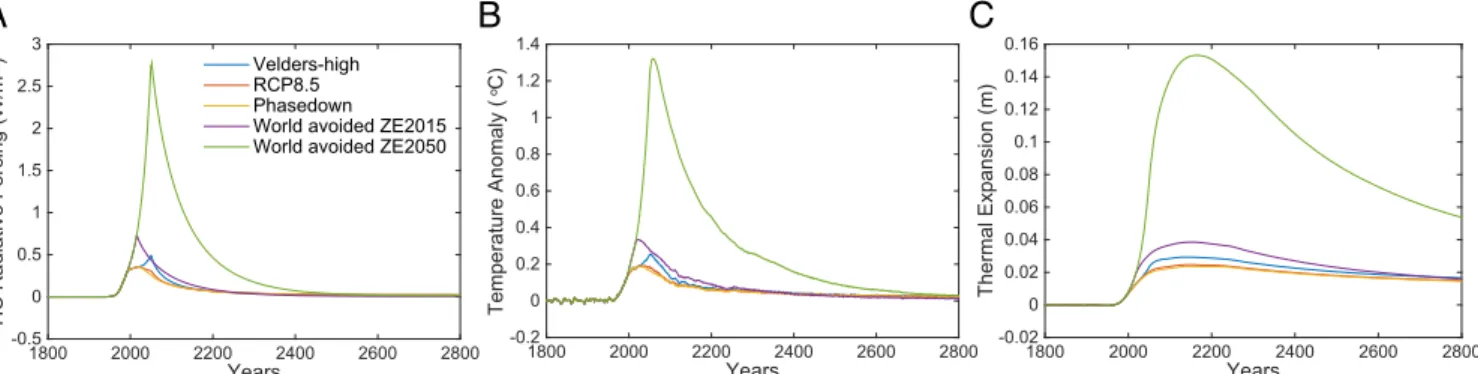
contribution from HCs if policies to phase down the consumption of HFCs were to be implemented using the“Phasedown” scenario developed by Rigby et al. (23), whereby overall HC RF decreases from 0.35 Wm−2in 2012 to 0.26 Wm−2in 2050, compared with a more modest decrease to 0.31 Wm−2in 2050 under RCP8.5 (Fig. 2A). We compare these thermal expansion contributions to two “no-HFC policy” scenarios, RCP8.5 and the high-end HC RF sce-nario discussed in Velders et al. (24); referred to as“Velders-high” (year-2050 RF of 0.49 W/m2). As in the simulations described pre-viously, HC RF follows these scenarios to 2050, after which emis-sions of all gases are eliminated. By year 2550 (500 y after emisemis-sions stop), TSLR due to HCs is similar across scenarios, indicating that by that time, the effect of HFC policies is small (<0.3 cm).

An interesting question is how ocean thermal expansion would have evolved had the ozone-depleting CFCs and HCFCs not been phased out under the Montreal Protocol. Such “world-avoided” scenarios have been explored for ozone depletion, RF, and surface temperature by several groups (e.g., refs. 25–27), but previous studies have not investigated the effect on TSLR. Here, we force the UVic ESCM using a scenario with RF from ozone-depleting substances (including CFCs, CH3CCl3, and CCl4)

growing at an adopted rate of 4% per year (about the growth rate in the 1980s) after the late 1980s [when the Montreal Pro-tocol was signed and entered into force (23)]. We hold the RF of HFCs, HCFCs, and perfluorocarbons constant at year-1989 levels because several of these gases were phased in as substitutes for CFCs. Emissions of all HCs are then set to zero in year 2015 or 2050. In these two world-avoided scenarios, HC RF reaches peak values of 0.71 W/m2in 2015 and 2.7 W/m2in 2050, respectively, compared with a peak value of 0.35 W/m2in the reference RCP8.5 scenario. This RF results in additional peak warming relative to the year 1800 of 0.3 °C and 1.3 °C, respectively (RCP8.5: 0.2 °C). Additional TSLR is 3.7 and 13.8 cm by 2100, respectively, and continuing contributions occur for centuries thereafter. The UVic ESCM overestimates ocean heat uptake over the historical period and is at the higher end of the range of ocean heat uptake (and hence TSLR) projections spanned by EMICs (9). To quantify the uncertainty in the TSLR rise estimates given above, we scale these estimates with the ocean heat-uptake efficiencies (defined as ocean heat uptake per degree surface air warming) of Climate Model Intercomparison Project 5 (CMIP5) models (28). This scaling gives a TSLR range of 1.2–3.7 and 4.5–14 cm for world-avoided sce-narios with HC RF zeroed in 2015 and 2050, respectively. Note that because of the high ocean heat-uptake efficiency of the UVic ESCM, the TSLR estimates presented in this study are at the upper end of this range.

A

B

C

Fig. 2. Climate response for scenarios with high (Velders-high), medium (RCP8.5), and low (Phasedown) HC (includes HFC, HCFC, CFC, and perfluorocarbon) RF to 2050 and exponentially declining RF thereafter. Results are also shown for two world-avoided scenarios with RF of ozone-depleting substances in-creasing at 4% per year (the increase rate before implementation of the Montreal Protocol) to 2015 and 2050 and zero emissions thereafter. The response to HC forcing is calculated as the difference between CO2+ N2O+ CH4+ HC and CO2+ N2O+ CH4simulations. (A) HC RF. (B) SAT difference. (C) Ocean thermal

expansion difference.

SU

Dependence on Emission Scenario. In the following, we further examine the dependence of the warming and TSLR commitment on the emissions scenario for a GHG with a very long (millennial) atmospheric lifetime (CO2) and one with a relatively short lifetime

(CH4). We explore the climate response to emission scenarios

following RCP8.5 to year 2050, 2100, and 2150 and zero emis-sions thereafter for a case with CO2emissions only and one with

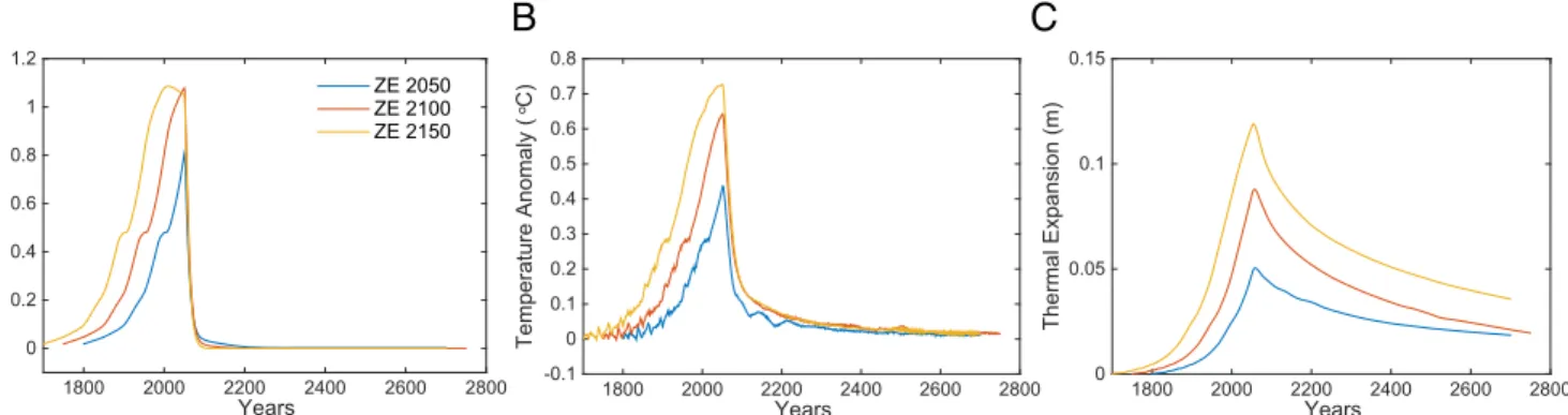
CO2and CH4emissions. The climate response to CH4(Fig. 3)

is calculated as the difference between the CO2+ CH4 and

CO2-only cases.

These experiments demonstrate the critical importance of ear-lier actions if future warming and sea-level rise are to be limited. For CO2, the longer emissions are sustained, the larger the fraction

of total emissions remaining in the atmosphere 500 y after emis-sions are set to zero (Fig. S2) (6, 8). SAT continues to increase after CO2emissions cease, with the warming“commitment”

in-creasing if emissions are sustained longer (9). The thermal expan-sion commitment also increases for scenarios with longer sustained CO2emissions.

For CH4, the fraction of RF persisting at a given time after

emissions are zeroed is the same for all scenarios (by definition) (Fig. 3). The SAT decline is also very similar between scenarios, with 14–17% of the peak warming remaining 100 y after emis-sions cease. The decline in thermal expansion, on the other hand, is emissions scenario-dependent: the longer emissions follow RCP8.5 before they are set to zero, the larger the TSLR persisting at any given time. In relative terms, the thermal expansion per-sisting 200 y after emissions are set to zero is 60, 53, and 54% of the peak for scenarios with emissions set to zero in 2050, 2100, and 2150, respectively. Interestingly, the fraction of the peak TSLR persisting is largest in the scenario with the lowest duration/ total amount of emissions. We attribute these differences in the timing of heat release to differences in the Atlantic Meridional Overturning Circulation (AMOC) in the climate state from which the CH4forcing is applied (recall that the three scenarios also

differ in terms of atmospheric CO2 concentration; Fig. S2A).

For scenarios with longer sustained GHG emissions, the AMOC weakens more in this model, resulting in less heat being mixed into the deep ocean during periods of increasing RF but also allowing for a faster release of the heat during periods of de-clining RF.

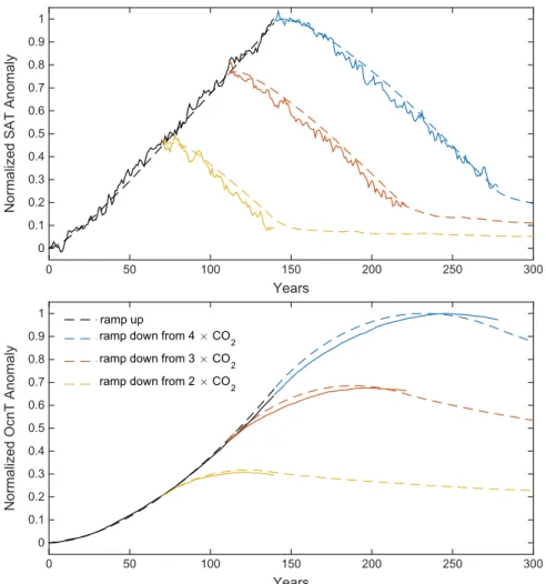
Ocean heat uptake and release at a given time is set by the time scale of mixing of heat into/out of the deep ocean, which is de-pendent on a model’s mixing parameterization and ocean circu-lation response. Both differ widely between models. In particular, the ability of EMICs to correctly simulate the time scale of ocean heat uptake has been questioned (29).Fig. S3compares the sur-face air and ocean temperature (a proxy for TSLR) responses of

the UVic ESCM to those of the Hadley Centre Earth System Model (HadGEM2) for a set of idealized scenarios with a 1% per year CO2increase followed by a 1% per year decrease (30, 31).

We find that the time scales of surface air and ocean-temperature response to rapidly declining CO2forcing are very similar between

the two models, suggesting that the centennial time scale of TSLR reversibility for short-lived GHGs found in this study is robust across models of different complexity.

Given concerns about challenges and progress in limiting emissions of CO2at a global scale, and the longevity of CO2in

the atmosphere, technologies that seek to remove CO2

artifi-cially from the atmosphere have been discussed (32). Artificial carbon dioxide removal (referred to as“CDR”) would lead to a faster decline in CO2RF, potentially allowing for the reversal

of CO2-induced climate change and return to a given climate

target (such as the 1.5 and 2 °C goals included in the Paris Agreement) after overshoot. The results presented here for short-lived climate forcers indicate that although CDR could be effective at restoring global SAT to a target level within de-cades, it would take centuries to reverse the associated thermal expansion (33).

Physical Processes That Determine Rate of Thermal Expansion.We next develop a simple model to explore the TSLR response during periods of declining RF. It has been suggested that thermal ex-pansion in response to increasing RF is approximately proportional to the time-integrated RF (3), which in turn can be used to justify empirical approaches that assume the rate of sea-level rise to scale with atmospheric temperature anomaly (18, 19). Empirical for-mulations have the advantages of simplicity and consideration of ice loss along with thermal expansion. However, here, we show that additional information is needed to capture the thermal expansion during periods of strongly declining RF, as is the case for CH4after

elimination of emissions: time-integrated RF approaches a con-stant level shortly after emissions cease, but rather than remaining constant, modeled thermal expansion declines significantly after emissions stop in all scenarios (Fig. 3). We expand the formulation of Bouttes et al. (3) by introducing an additional term to include the important effect of radiative damping through energy loss to space: η = α Z RF  dt − β Z _​ ðT − T0Þdt, [1]

whereη is ocean thermal expansion, RF is total RF (in W/m2_),

ΔT = T − T0is the temperature anomaly relative to a reference

year (denoted year 0), andα, β are constants (see below).

A

B

C

Fig. 3. Climate response computed with the UVic ESCM for scenarios with CH4emissions following RCP8.5 to year 2050, 2100, 2150, and zero anthropogenic

emissions (ZE) thereafter. Variables are calculated as differences between CO2+ CH4and CO2-only simulations and are aligned at the time emissions are set to

zero (which results in a shift by 50 and 100 y in the ZE2100 and ZE2150 scenarios, respectively). (A) CH4RF. (B) SAT anomaly relative to year 1800. (C) Ocean

thermal expansion relative to year 1800.

By taking the time derivative, one obtains a useful expression for the rate of TSLR:

dη

dt= αRF − βΔT. [2] The ratio β/α has units of W·m−2·K−1, the same units as the climate-feedback parameter (denoted asλÞ. The equivalence be-tween the ratio β/α and the climate-feedback parameter can easily be seen by assuming that the rate of thermal expansion is proportional to the rate of ocean heat-uptakeN (dη/dt = γN, whereγ is a proportionality constant) and comparing the resulting expression to a zero-dimensional global Earth energy balance model:

N = RF − λΔT. [3]

Using this simple energy balance model and assuming a repre-sentative value ofλ allows one to directly predict the evolution of TSLR for given climate scenarios, including those where RF is strongly decreasing.

The TSLR predicted by the simple model given in Eq.2 agrees well with the thermal expansion simulated by the UVic ESCM during periods of both increasing and decreasing RF, as illustrated in Fig. 4 for the scenario with zero emissions after year 2100. Analysis of the terms in Eq. 3 gives insight into the different thermal expansion responses to CO2and CH4RF (Fig. 4A and

C). For CO2, RF declines after emissions are set to zero, whereas

SAT and hence radiative damping (λΔT) continues to increase slightly; RF remains larger thanλΔT for CO2in Fig. 4A, although

the difference declines toward the end of the simulation. There-fore, the rate of thermal expansion remains positive after emis-sions cease, and the expansion declines over time (Fig. 4B). For CH4, RF declines rapidly after emissions are set to zero (reflecting

the short residence time of CH4). SAT lags the decline in RF but

also decreases. The net result is that RF becomes smaller than λΔT shortly after emissions cease, such that the rate of thermal expansion becomes negative (Fig. 4 C and D). These physical

principles demonstrate why geoengineering proposals that could decrease atmospheric temperature to a target level within de-cades, such as CDR or solar radiation management schemes, would also imply a much slower decline in sea level (33).

Bouttes et al. (3) also considered a zero-dimensional energy balance model (Eq.2), but their formulation does not include the thermal expansion response during periods of declining RF. The reason is that they assumed the rate of ocean heat-uptake N is always proportional to temperature (N = κΔT, where κ is the ocean heat-uptake efficiency). This linear assumption is justified for in-creasing but not for dein-creasing RF, whenN can become negative.

Observational constraints on sea-level rise using historical data have been tested in previous studies (e.g., refs. 34 and 35) with paleoclimate records. However, these semiempirical approaches were calibrated assuming sea-level rise will tend toward its long-term (multimillennial) global temperature relationship in the presence of short-term forcing; they do not include a forcing term based on Earth’s energy balance, and they have not been tested under periods of sharply declining RF (such as those that occur if CH4emissions suddenly cease). Our method is valuable because it

is generalizable for any climate scenario and model given the value of λ, which allows us to separate the physical contributions to TSLR from energy input to the ocean and radiative damping. Conclusions

We have used an EMIC to elucidate thermal sea-level responses to changes in short-lived GHGs and have described the re-sponses’ contrasts and similarities with those obtained for CO2.

We have only considered thermal sea-level rise and have neglected contributions from glaciers and ice-sheet melt. On very long (>1,000 y) time scales, these processes are expected to dominate contributions to the global GHG commitment to sea-level rise, and the relationship between ice-melt contributions and ther-mal expansion is only quasilinear (34).

Our results show that centuries of TSLR are to be expected if the emissions of CH4 or other short-lived anthropogenic GHGs

such as HFCs were to cease, due to the slow time scales of release

A

C

D

B

Fig. 4. Energy balance terms and rate of ocean thermal expansion for scenarios with CO2(A and B) and CH4(C and D) emissions following RCP 8.5 to year 2100

and zero anthropogenic emissions thereafter. The simple energy balance model terms are shown by the blue curves in B and D, which are scaled for comparison with the full model calculation (red curves). The climate response to CH4forcing is calculated as the difference between CO2+ CH4and CO2-only simulations. In

these calculations, the climate-feedback parameterλ = β=α is set to 1.0 W/m2_{/K, the value diagnosed in the standard configuration of the UVic ESCM.}

SU

of heat from the atmosphere/ocean system. Thus, although sea-level rise due to short-lived GHGs can be expected to become small compared with CO2’s influence on sea level within a few hundred

years if anthropogenic emissions of both were to cease, the climate impacts of short-lived GHGs are far longer-lasting than would be implied by their atmospheric lifetimes alone. A simple energy bal-ance model has been used to elucidate the factors that influence the rate and magnitude of sea-level rise regardless of whether RF and atmospheric temperatures are increasing or decreasing. This study shows that radiative damping and ocean heat uptake are important in determining the temporal evolution of sea-level rise and that the rate of sea-level rise can be readily related to the climate-feedback parameter.

CFCs, HCFCs, and HFCs are much shorter-lived than CO2and

yet cause sea-level rise that also persists for centuries. We have shown that choices made to phase out the CFCs and HCFCs during the 20th century under the Montreal Protocol have avoided a considerable amount of TSLR. If the CFCs and HCFCs had not been phased out until 2050, an additional 13.8 cm (4.5–14.0 cm) of TSLR would be expected by the end of this century, with continu-ing contributions for many centuries to come; this findcontinu-ing attests to the long-term value of the Montreal Protocol in avoiding a world with significantly higher sea levels.

The primary policy conclusion of this study is that the long-lasting nature of sea-level rise heightens the importance of earlier

mitigation actions—even in the case of a short-lived substance such as CH4, HFCs, etc. Our work also indicates that longer-term

sea-level rise impacts should be considered if the climate impli-cations of geoengineering proposals that seek to reduce RF or atmospheric temperatures are to be fully evaluated. As can be seen in Fig. 3 for CH4, a scenario that reduces atmospheric temperature

cannot be assumed to simultaneously eliminate future sea-level rise, due to the time scales associated with release of stored energy in the ocean.

Methods

We use version 2.9 of the UVic ESCM (8, 36), a model of intermediate com-plexity. This version of the UVic ESCM includes a 3D ocean GCM, coupled to a dynamic-thermodynamic sea-ice model and a single-layer energy–moisture balance model of the atmosphere with dynamical feedbacks. The physical climate model is fully coupled to carbon-cycle components on land and in the ocean. Further details regarding the model and simulation protocol are pro-vided inSI Methods.

ACKNOWLEDGMENTS. We thank W. Morgenstern for preparing the RF input and carrying out part of the model simulations with the UVic ESCM. This research was enabled in part by computing resources provided by Westgrid and Compute Canada. K.Z. acknowledges support from the Natural Sciences and Engineering Research Council of Canada Discovery Grant and Undergrad-uate Student Research Assistant Programs. D.M.G. is partly supported by a National Aeronautics and Space Administration fellowship.

1. Contribution of Working Group I to the Fifth Assessment Report of the In-tergovernmental Panel on Climate Change (2013) Climate Change 2013: The Physical Science Basis, eds Stocker TF, Qin D (Cambridge Univ Press, Cambridge, UK). 2. Solomon S, et al. (2010) Persistence of climate changes due to a range of greenhouse

gases. Proc Natl Acad Sci USA 107(43):18354–18359.

3. Bouttes N, Gregory JM, Lowe JA (2013) The reversibility of sea level rise. J Clim 26: 2502–2513.

4. United Nations (2015) Adoption of the Paris agreement. Framework Convention on Climate Change. Available at https://unfccc.int/resource/docs/2015/cop21/eng/l09.pdf. Accessed December 22, 2016.

5. Matthews HD, Caldeira K (2008) Stabilizing climate requires near-zero emissions. Geophys Res Lett 35:L04705.

6. Plattner GK, et al. (2008) Long-term climate commitments projected with climate-carbon cycle models. J Clim 21:2721–2751.

7. Solomon S, Plattner G-K, Knutti R, Friedlingstein P (2009) Irreversible climate change due to carbon dioxide emissions. Proc Natl Acad Sci USA 106(6):1704–1709. 8. Eby M, et al. (2009) Lifetime of anthropogenic climate change: millennial time-scales

of potential CO2and surface temperature perturbations. J Clim 22:2501–2511.

9. Zickfeld K, et al. (2013) Long-term climate change commitment and reversibility: an EMIC intercomparison. J Clim 26:5782–5809.

10. Lowe JS, et al. (2009) How difficult is it to recover from dangerous levels of global warming? Environ Res Lett 4:1–9.

11. Frölicher TL, Joos F (2010) Reversible and irreversible impacts of greenhouse gas emissions in multi-century projections with the NCAR global coupled carbon cycle-climate model. Clim Dyn 35:1439–1459.

12. Gillett NP, Arora V, Zickfeld K, Marshall S, Merryfield WJ (2011) Ongoing climate change following a complete cessation of carbon dioxide emissions. Nat Geosci 4: 83–87.

13. Zickfeld K, Arora VK, Gillett NP (2012) Is the climate response to carbon emissions path dependent? Geophys Res Lett 39:L05703.

14. Molina M, et al. (2009) Reducing abrupt climate change risk using the Montreal Protocol and other regulatory actions to complement cuts in CO2emissions. Proc Natl

Acad Sci USA 106(49):20616–20621.

15. Ramanathan V, Xu Y (2010) The Copenhagen Accord for limiting global warming: criteria, constraints, and available avenues. Proc Natl Acad Sci USA 107(18): 8055–8062.

16. Shindell D, et al. (2012) Simultaneously mitigating near-term climate change and improving human health and food security. Science 335(6065):183–189.

17. Hu A, Xu Y, Tebaldi C, Washington WM, Ramanathan V (2013) Mitigation of short lived climate pollutants slows sea level rise. Nat Clim Chang 3:730–734.

18. Rahmstorf S (2007) A semi-empirical approach to projecting future sea-level rise. Science 315(5810):368–370.

19. Vermeer M, Rahmstorf S (2009) Global sea level linked to global temperature. Proc Natl Acad Sci USA 106(51):21527–21532.

20. Archer D, Kheshgi H, Maier-Reimer E (1997) Multiple timescales for neutralization of fossil fuel CO2. Geophys Res Lett 24:405–408.

21. Joos F, et al. (2013) Carbon dioxide and climate impulse response functions for the computation of greenhouse gas metrics: a multi-model analysis. Atmos Chem Phys 13: 2793–2825.

22. Myhre G, et al. (2013) Anthropogenic and natural radiative forcing. Climate Change 2013: The Physical Science Basis, eds Stocker TF, Qin D (Cambridge Univ Press, New York), 659–740.

23. Rigby M, et al. (2014) Recent and future trends in synthetic greenhouse gas radiative forcing. Geophys Res Lett 41:2623–2630.

24. Velders GJM, Fahey DW, Daniel JS, McFarland M, Andersen SO (2009) The large contribution of projected HFC emissions to future climate forcing. Proc Natl Acad Sci USA 106(27):10949–10954.

25. Velders GJM, Andersen SO, Daniel JS, Fahey DW, McFarland M (2007) The importance of the Montreal Protocol in protecting climate. Proc Natl Acad Sci USA 104(12): 4814–4819.

26. Newman PA, et al. (2009) What would have happened to the ozone layer if chloro-fluorocarbons (CFCs) had not been regulated? Atmos Chem Phys 9:2113–2128. 27. Garcia RR, Kinnison DE, Marsh DR (2012)“World avoided” simulations with the

Whole Atmosphere Community Climate Model. J Geophys Res 117:D23303. 28. Kuhlbrodt T, Gregory JM (2012) Ocean heat uptake and its consequences for the

magnitude of sea level rise and climate change. Geophys Res Lett 9:L18608. 29. Frölicher TL, Paynter DJ (2015) Extending the relationship between global warming

and cumulative carbon emissions to multi-millennial timescales. Environ Res Lett 10: 75002.

30. Boucher O, et al. (2012) Reversibility in an Earth System model in response to CO2

concentration changes. Environ Res Lett 7:024013.

31. Zickfeld K, MacDougall A, Matthews HD (2016) On the proportionality between global temperature change and cumulative CO2 emissions during periods of net negative CO2 emissions. Environ Res Lett 11:055006.

32. National Research Council (2015) Climate Intervention: Carbon Dioxide Removal and Reliable Sequestration (National Academies Press, Washington, DC).

33. Tokarska KB, Zickfeld K (2015) The effectiveness of net negative carbon dioxide emissions in reversing anthropogenic climate change. Environ Res Lett 10:094013. 34. Levermann A, et al. (2013) The multimillennial sea-level commitment of global

warming. Proc Natl Acad Sci USA 110(34):13745–13750.

35. Mengel M, et al. (2016) Future sea level rise constrained by observations and long-term commitment. Proc Natl Acad Sci USA 113(10):2597–2602.

36. Weaver AJ, et al. (2001) The UVic Earth System Climate Model: model description, climatology, and applications to past, present and future climates. Atmos Ocean 39: 361–428.

37. Eby M, et al. (2013) Historical and idealized climate model experiments: an in-tercomparison of Earth system models of intermediate complexity. Clim Past 9: 1111–1140.

38. Arora V, et al. (2013) Carbon-concentration and carbon-climate feedbacks in CMIP5 Earth system models. J Clim 26:5289–5314.

39. Meinshausen M, et al. (2011) The RCP greenhouse gas concentrations and their ex-tensions from 1765 to 2300. Clim Change 109:213–241.

40. Prinn RG, et al. (2000) A history of chemically and radiatively important gases in air deduced from ALE/GAGE/AGAGE. J Geophys Res 105:17,751–17,792.

Supporting Information

Zickfeld et al. 10.1073/pnas.1612066114

SI Methods

We use version 2.9 of the UVic ESCM (8, 36), a model of in-termediate complexity with a horizontal grid resolution of 1.8°× 3.6°. This version of the UVic ESCM includes a 3D ocean GCM with isopycnal mixing and a Gent–McWilliams parameterization of the effect of eddy-induced tracer transport. For diapycnal mixing, a Bryan and Lewis profile of diffusivity is applied, with a value of 0.3× 10−4m2_·s−1_{in the pycnocline. The ocean model is}

coupled to a dynamic–thermodynamic sea-ice model and a single-layer energy–moisture balance model of the atmosphere with dynamical feedbacks (36). The atmospheric model does not sim-ulate clouds, and precipitation is assumed to occur when relative humidity exceeds 85%. The model includes a parameterization of water vapor/planetary longwave feedbacks, and the RF associated with changes in atmospheric CO2and other GHGs is prescribed

as a modification of the planetary longwave radiative flux. The land surface and vegetation are represented by a simplified ver-sion of the Hadley Centre’s land-surface scheme (Met Office Surface Exchange Scheme) coupled to the dynamic vegetation model TRIFFID (Top-Down Representation of Interactive Fo-liage and Flora Including Dynamics). Ocean carbon is simulated by means of an Ocean–Carbon Cycle Model Intercomparison Project-type inorganic carbon-cycle model and a marine ecosys-tem/biogeochemistry model solving prognostic equations for nu-trients, phytoplankton, zooplankton, and detritus. The version of the UVic ESCM used here includes a marine sediment compo-nent (8). CO2 can be specified to the model either in terms of

emissions or atmospheric concentrations. The model does not include an atmospheric chemistry module; non-CO2GHGs are

specified as RF.

The UVic ESCM took part in numerous model intercomparison projects, including the EMIC Intercomparison in support of the Fifth Assessment Report (AR5) of the Intergovernmental Panel on Climate Change (EMIC AR5) (9, 37). The model’s standard climate sensitivity is 3.5 °C for a doubling of the preindustrial atmospheric CO2 concentration (37). The model overestimates

thermal sea-level rise over the historical period and is at the higher

end of the range of thermal sea-level rise projections spanned by EMICs (9). In terms of carbon cycle response to CO2and climate

change, the UVic ESCM lies in the middle of the range of re-sponses of EMICs and complex Earth system models (37, 38).

Several simulations were run with the UVic ESCM, with dif-ferent combinations of GHGs and difdif-ferent times at which GHG emissions were set to zero. These simulations were initialized from a preindustrial equilibrium state of the model. CO2-only

simula-tions were forced with historical CO2concentrations to 2010 and

RCP8.5 and ECP8.5 CO2concentrations from 2010 to 2300 (39).

CO2emissions were then set to zero at different times along this

trajectory: in 2050, 2100, and 2150. CO2concentrations from these

simulations were used to force runs with different combinations of non-CO2forcings: CH4, CH4+ N2O and CH4+ N2O+ HCs. HCs

here include CFCs, HCFCs, HFCs, and perfluorinated gases. RF of CH4and N2O followed observation-based values to 2010 and

RCP8.5 and ECP8.5 values thereafter. The decline in RF after emissions of these gases were set to zero was calculated using standard formulae (see, for example, supplementary material 8.SM.3 of ref. 22). For HCs, we used observations-based RF to 2010 [Advanced Global Atmospheric Gases Experiment (40)] and three different RF scenarios up to 2050 spanning a range of plau-sible future emissions of these gases: a high scenario from Velders et al. (24) (“Velders-high”), a medium scenario (RCP8.5), and a low scenario proposed by Rigby et al. (23), which assumes that policies to phase down the consumption of HFCs are implemented (Phasedown). After 2050, HC RF was prescribed to decline ex-ponentially according to each gas’s atmospheric lifetime as given in appendix 8.A of ref. 22. In addition, we forced the model with two world-avoided scenarios, whereby RF of ozone depleting sub-stances (CFCs, CH3CCl3, and CCl4) increases at 4% per year (the

rate of increase in the 1980s before ratification of the Montreal Protocol), and RF of HFCs and HCFCs is held constant at year-1989 levels. Emissions of these gases are assumed to stop after 2015 or 2050 and RF to decline exponentially. This simulation also includes RF from CO2, CH4, and N2O evolving as in the year-2050

Fig. S1. Linearity of SAT (A) and thermal sea-level-rise (B) responses associated with CH4emissions. CH4-induced responses are diagnosed from simulations

with CH4RF applied in isolation or from differences between simulations with different combinations of GHGs. Results are shown for a scenario with emissions

following RCP8.5 to year 2050, with zero anthropogenic emissions thereafter (ZE2050). TSLR is slightly larger and takes slightly longer to reverse if CH4is

emitted in isolation, than if it is emitted simultaneously with CO2, which has a much larger RF (Fig. S2). This difference in TSLR is due to differences in ocean

heat uptake at low and high RF: when only CH4is emitted, the ocean is less stratified and more heat is taken up, resulting in a slightly lower SAT and slightly

larger thermal expansion.

Fig. S2. Climate response computed with the UVic ESCM for a scenario with emissions of CO2and CH4, following RCP8.5 to year 2050, 2100, 2150, and with

zero anthropogenic emissions (ZE) thereafter. (A) Atmospheric CO2concentration. (B) SAT anomaly relative to year 1800. (C) Ocean thermal expansion relative

to year 1800. (D) Total RF. (E) Rate of SAT change. (F) Rate of ocean thermal expansion. Solid lines refer CO2-only simulations; dashed lines refer to CO2+ CH4

simulations.

Fig. S3. Comparison of SAT (Top) and ocean-temperature (Bottom) response for the UVic ESCM (dashed lines) and the HadGEM2 ESM (solid lines). Results are shown for idealized scenarios with a 1% per year increase in atmospheric CO2(“ramp up”), followed by a 1% per year CO2decrease (“ramp down”) from 2×

CO2, 3× CO2, and 4× CO2(1, 2). For better comparison of the response time scales involved, temperature anomalies are normalized to the peak value in the