Evidence of different ocean responses to atmospheric pressurevariations in the Atlantic, Indian and Pacific Basins as deduced fromERS-2 altimetric data

HAL Id: hal-00317221

https://hal.archives-ouvertes.fr/hal-00317221

Submitted on 1 Jan 2004

HAL is a multi-disciplinary open access

archive for the deposit and dissemination of

sci-entific research documents, whether they are

pub-lished or not. The documents may come from

teaching and research institutions in France or

abroad, or from public or private research centers.

L’archive ouverte pluridisciplinaire HAL, est

destinée au dépôt et à la diffusion de documents

scientifiques de niveau recherche, publiés ou non,

émanant des établissements d’enseignement et de

recherche français ou étrangers, des laboratoires

publics ou privés.

pressurevariations in the Atlantic, Indian and Pacific

Basins as deduced fromERS-2 altimetric data

J. Gómez-Enri, P. Villares, M. Bruno, M. Catalán

To cite this version:

J. Gómez-Enri, P. Villares, M. Bruno, M. Catalán. Evidence of different ocean responses to

atmo-spheric pressurevariations in the Atlantic, Indian and Pacific Basins as deduced fromERS-2 altimetric

data. Annales Geophysicae, European Geosciences Union, 2004, 22 (2), pp.331-345. �hal-00317221�

Annales Geophysicae (2004) 22: 331–345 © European Geosciences Union 2004

Annales

Geophysicae

Evidence of different ocean responses to atmospheric pressure

variations in the Atlantic, Indian and Pacific Basins as deduced from

ERS-2 altimetric data

J. G´omez-Enri1, P. Villares1, M. Bruno1, and M. Catal´an1

1_{Applied Physics Department (CASEM), University of Cadiz, Pol´ıgono R´ıo S. Pedro s/n. 11510. Puerto Real, Spain}

Received: 17 September 2002 – Revised: 2 February 2003 – Accepted: 23 June 2003 – Published: 1 January 2004

Abstract. The exponential increase in the use of altimeter

data in oceanographic studies in the past two decades has im-proved the knowledge of the processes that govern the inter-action between the ocean and the atmosphere. One of these processes is the response of the ocean to atmospheric pres-sure variations, which has been deeply analysed in the past. That response is based on the isostatic assumption used to establish a standard correction for altimetric purposes, the Inverse Barometer Correction (IBC). As a general rule, the ocean goes up/down 1 cm when the atmospheric pressure goes down/up 1 mbar. However, in light of recent works in some oceanic regions, discrepancies arise when the real re-sponse is compared to the hypothetical one. It is important to quantify this discrepancy, in order to improve the accuracy of the correction, which is one of the most significant geophysi-cal corrections applied to altimeter records. Some aspects of this response remain unclear, such as the real space-temporal scales where IBC can be applied, the influence of wind, non-isostatic atmospheric pressure-driven signals, and the effect of aliasing from high frequency signals. This paper is an at-tempt to gain insight into this phenomenon. The data used are the residuals obtained between sea surface heights from the ERS-2 altimeter and the outputs of a global barotropic ocean model. Significant departures from the hypothetical isostatic response in all data series (spatial and temporal do-main) have been found, especially in the case of altimeter records. By applying the collinear track method, we observe that the estimated Atlantic Ocean response is quite similar to the one deduced from the isostatic assumption at all lat-itudinal bands. Nonetheless, the Indian and Pacific Oceans show important departures from the hypothetical value at low latitudes. Results obtained with the crossover track method show important deviations at low latitudes in the three basins. In order to understand why the Atlantic Ocean response is different from the one obtained in the other two, we can infer some explanations based on the interaction of seasonal and intraseasonal signals with the isostatic one.

Correspondence to: J. G´omez-Enri (jesus.gomez@uca.es)

Key words. Meteorology and atmospheric dynamics (ocean-atmosphere interactions). Oceanography: physical (sea level variations; remote sensing, instruments and techniques)

1 Introduction

Sea level is one of the most important variables in ocean dy-namic studies. In general, in sea level measurements there is some temporal and spatial variability, mainly due to fluctu-ations in surface wind stress, atmospheric pressure and sur-face heat fluxes in the atmosphere-ocean intersur-face, as well as large-scale water mass transport (Gill and Niiler, 1973).

Traditionally, the ocean response to atmospheric surface pressure fluctuations has been a matter of investigation for the scientific community dedicated to oceanographic stud-ies: Lubbock (1836); Ross (1854); Close (1918). In fact, Rossiter (1962) and Roden (1966) note that the first inves-tigations were made for Gissler (1747). Using records of sea level and atmospheric pressure, Ross‘(1854) found that an increase (decrease) of 1 mbar in the atmospheric pressure produced a decrease (increase) of approximately 1 cm in the sea level. This behaviour has been called the Inverse Barom-eter approximation or simply, the Isostatic Assumption (Gill and Niiler, 1973).

Since the launch of environmental satellites, especially in the past decade, the study of ocean dynamics has become one of the main applications, and the Radar Altimeter (hereafter referred to as RA) is one of the instruments with the best re-sults. Basically, RA measures the height between the satellite centre of mass and the surface sea level (“Range”). Know-ing the distance between the satellite and a reference system (“Altitude”), we can infer the height between the sea level and this reference system. This height is commonly called “Sea Surface Height” (hereafter referred to as SSH). In order to isolate the dynamic part of the ocean signal, some instru-mental and geophysical corrections have to be applied to the measurement made by the RA. The unique character of sea level, being a surface signal, yet reflecting the state of the

ocean at depths, makes satellite altimetry a powerful tool for studying global ocean variabilities (Wunsch and Stammer, 1997). In fact, one of the advantages of satellite oceanog-raphy is its potential for global monitoring (Cheney et al., 1983).

One of the geophysical phenomena that we must eliminate from altimeter records is the ocean’s compensation for atmo-spheric pressure variations, the so-called Inverse Barometer Correction (hereafter referred to as IBC). This correction is based on the above mentioned Isostatic Assumption. After the orbit and ocean tide corrections, IBC is the most ener-getic correction applied to the data. Neither tides nor IBC are “corrections” in the sense of modifying altimeter mea-surements to yield the correct sea level, but rather an attempt to remove “known” oceanic signals to better determine the global ocean dynamic topography records from altimeters.

The suitability of the application of IBC to altimeter records has been previously analysed by some authors, by us-ing Geosat data (van Dam and Wahr, 1993-hereafter referred to as vDW93) and mainly TOPEX-Poseidon data (Fu and Pi-hos, 1994; Gaspar and Ponte, 1997, 1998; Ponte and Gaspar, 1999;) and more recently, Mathers and Woodworth (2001) (hereafter respectively referred to as FP94, GP97, PG99 and MW01). Nevertheless, little is done with ERS-1 and ERS-2 data (G´omez-Enri et al., 2001: GE01).

With the aim to analyse the real response of the ocean to at-mospheric pressure variations, we are going to use two differ-ent and independdiffer-ent sources of information: ERS-2 altimeter data, provided by the Centre ERS d’Archivage et de Trait-ment (CERSAT) (European Space Agency) and the outputs of a global Ocean Barotropic Model (hereafter referred to as OBM), developed by the Jet Propulsion Laboratory (JPL) (National Aeronautics and Space Administration).

In the present paper we describe the sea surface response mentioned in the three main ocean basins: Atlantic, Indian and Pacific, by using ERS-2 altimeter data. In order to pre-pare the variables for the analyses, we used two different techniques: the collinear track and the crossover track tech-nique. We will start with the data processing. In the next section, we will present the results obtained by applying the techniques used to estimate the inverse barometer response: the simple linear regression analysis and the empirical or-thogonal function decomposition analysis. A discussion of the results obtained will finish the work.

2 Data processing

2.1 Altimeter data

The first step is to develop editing processes to eliminate bad data points with errors an order of magnitude larger than ERS altimeter precision. The criterion used was the number of 20-Hz elementary measurements used for computing the 1-Hz measurement (Nval), which represents the number of elementary measurements declared “ocean” (Nval = 20) by OIP (Ocean Intermediate Product) processing. As suggested

in the User Manual (CERSAT, 1996; hereafter referred to as C96), only data with Nval ≥ 17 were considered as valid measurements. Also considered was the Measurement Con-fidence Data (MCD) of each field read (C96).

The next step is the estimation of SSH by subtracting the altimeter range and the environmental corrections from the altimeter altitude. We must note that the range includes all the suggested instrumental corrections (C96). As far as the environmental corrections are concerned, they were applied to remove the effects of the troposphere, ionosphere, tides and sea state bias (corrected as suggested by Gaspar and Ogor, 1996), including the scanning point target and the ul-tra stable oscillator corrections (Benveniste, 1996a, 1996b; Loial, 1996), and the time tag bias correction (Dorandeu and Stum, 1996). Finally, the original altitude produced by the German Processing and Archiving Facility (D-PAF), with an accuracy between 10 and 15 cm, was replaced by the one produced at the Delft Institute of Technology (DEOS) with an accuracy of around 5 cm (Scharroo and Visser, 1998).

Atmospheric pressure (Ps) is directly inferred through the dry tropospheric correction by inverting the Saastamoinen formula (Saastamoinen, 1972). Finally, the correction IBC can be obtained by applying the isostatic assumption as:

I BC(cm) = BF (P s − Pa). (1)

Pa is the spatial average of atmospheric pressure over the global ocean and BF determines the relation between atmo-spheric pressure variations and sea level fluctuations. It is usual to assume this value to be constant in time, considering that the variability of the spatial average may be small when considering the whole ocean (Ponte et al., 1991). Using the above mentioned assumption, this barometric factor should be close to 0.995 cm/mb (C96). A cubic spline interpolation was then applied, in order to align the common points from the ascending and descending collinear passes along perpen-diculars to the ground track, placing them to a fixed set of latitudinal spacing corresponding to 1-s intervals, i.e. 7 km along the track. This is necessary to ensure maximum preci-sion for accurate measurements of SSH and Ps. To accom-plish this, data were low-pass filtered using a 35-km median filter and a simple low-pass filter with a cut-off wavelength of 77 km.

Traditionally, direct use of SSH is avoided, because it con-tains non-desirable, very energetic signals (mainly the geoid variations), which are an order of magnitude higher than the ocean response in which we are interested. For this reason, it is preferable to eliminate these kinds of signals by using the difference between two measurements made at the same geographic point at two consecutive times (“Sea Level Anomaly”: SLA). Although there are other possibili-ties to obtain these differences, we have chosen two different methods: collinear track method and crossover track method (hereafter referred to as CT and XT). In this way, we build the difference in both methods as the quantity:

J. G´omez-Enri et al.: Different ocean responses to atmospheric pressure variations 333

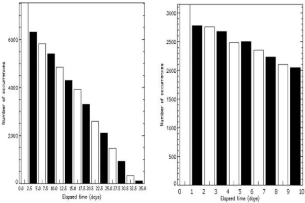
Fig. 1. Number of crossover points as a function of the elapsed time between the ascending and descending tracks (absolute value). (a) shows the number of crossovers in the complete time interval considering the same cycle for both track: 35 days. (b) shows the same,

but considering crossovers produced between 0 and 10 days.

where:

SSH: variable analysed,

8: latitude,

λ: longitude,

ti: time of each measurement.

tm=(t2−t1)/2. Mean time between the two measurements,

The atmospheric pressure differences (DSP) are obtained similarly as:

DSP (8, λ, tm) = Ps(8, λ, t1) − Ps(8, λ, t2). (3)

Now, let the SSH and Psvariables be written as:

SSH (8, λ, t ) = SSH0(8, λ, t ) + SSHm(t ) (4)

Ps(8, λ, t ) = Ps0(8, λ, t ) + Pa(t ), (5) where SSHm and Pa are respectively the globally averaged values of SSH and Ps but now having a slow variation with time variation; SSH0and P_s0are the departures from their re-spective averages. The substitution of Eqs. (4) and (5) into Eqs. (2) and (3) leads to:

SLA(8, λ, tm) = [SSH0(8, λ, t1) − SSH0(8, λ, t2)]

+[SSHm(t1) − SSHm(t2)] (6)

DSP (8, λ, tm) + [Ps0(8, λ, t1) − Ps0(8, λ, t2)]

+[Pa(t1) − Pa(t2)] (7)

If SSHmand Paare assumed to show very slow variations with time, the last right-hand term in Eqs. (6) and (7) may be disregarded against the first ones. Therefore, we can expect that the variations with time of the spatially averaged signals do not affect to a great extent the BF estimates made with linear analysis techniques. Some tests performed by previous authors (GP97 and PG99) support this assumption.

We must point out some differences between CT and XT: first, the time elapsed between the two consecutive measure-ments (1t = |t1−t2|) is for CT. 35 days, while for XT it is

possible to choose different 1t, from 0 to 35 days (Fig. 1). If we select the complete set of crossover points, we obtain a mean 1t of approximately 11 days. Second, with CT we have global coverage with points homogeneously distributed at all latitudes, but in the case of XT there is a scarcity of points at low latitudes. This is not a limitation when us-ing ERS-2, as it is with TOPEX-Poseidon (MW01), since the number of points at these latitudes is enough to ensure a global coverage. In fact, the wide spatial distribution and number of ERS-2 crossover points allows us to select only those points where 1t is between 0 and 10 days, which pro-duces a mean 1t of 4 days. Finally, CT allows us to promote the ocean variability with frequencies closer to the Nyquist frequency of the satellite (f = 1/70 days−1). On the other hand, with XT we are promoting the variability with higher frequencies, concretely between (f = 1/22 days−1) and (f = 1/8 days−1). The two techniques proposed allow us to estimate the ocean response to atmospheric pressure

vari-Table 1. Number of crossover points when considering one

cy-cle of ERS-2 and Topex-Poseidon (T-P) and a time sampling,

1t ≤10 days. This time interval has been divided into sub-intervals with a one day width.

1t ERS-2 T-P [0, 1] 3147 ∼1400 [1, 2] 2777 ∼1250 [2, 3] 2756 ∼1100 [3, 4] 2678 ∼900 [4, 5] 2479 ∼800 [5, 6] 2502 ∼650 [6, 7] 2349 ∼500 [7, 8] 2230 ∼400 [8, 9] 2100 ∼200 [9, 10] 2046 ∼50

ations with three different 1t. So, we will be able to know if that response is or is not sensitive to the change in 1t. We consider that the method proposed by MW01, the parallel track method, is not necessary when using ERS-2, data due to the high spatial resolution of the crossover points.

Table 1 compares the number of crossover points be-tween ascending and descending tracks of ERS-2 (column 2) and TOPEX-Poseidon (column 3) satellites. In the case of ERS-2, only those intersections where 1t ≤ 10 days are considered. We present the results in sub-intervals of a one-day width. The number of points when using the ERS-2 data set is much higher than in the TOPEX-Poseidon data. 2.2 Global Ocean Barotropic Model data (OBM)

Aside from the altimeter data, we propose to estimate the ocean response to atmospheric pressure variations by using an independent source of data, such as the outputs of a near-global barotropic model (OBM). The model used in this work is a two-dimensional, 1.125-degree spatial resolution in both latitude and longitude, and has been thoroughly described in Ponte (1993) and Hirose et al. (2001). The baroclinic compo-nent has not been included. This model resolves the primitive equations of motion (Gill, 1982) considering two different forcing fields: wind stress and atmospheric pressure forcing at the sea surface, both obtained from NCEP (National Cen-ter for Environmental Prediction-NOAA).

The signal that is generated by the model may be decom-posed into four different components:

H (8, λ, t ) + hBI+hv+hp+hvp, (8) where subscript BI indicates the isostatic elevation due to atmospheric pressure and p and v indicate the ocean dy-namic components produced by atmospheric pressure and wind stress, respectively. The term hvpis referred to the part of the sea level response associated with one word the non-linear interaction between the wind and atmospheric pres-sure driven signals. We assume that the wind and

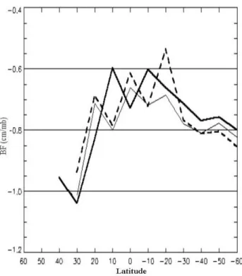
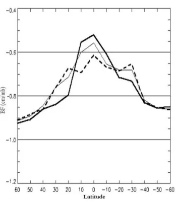
atmo-Fig. 2. Meridional distribution of the Barometric Factors (BF)

esti-mated using ERS-2 altimeter records, in the Atlantic Basin, consid-ering the three different time samplings used: 35 days (gross solid line), 11 days (thin solid line) and 4 days (dashed line).

spheric pressure driven sea level changes are generally an-ticorrelated and thereby tend to reduce the value of the lin-ear regression coefficient between sea level and atmospheric pressure (Ponte, 1994; vDW93). The original data set were re-sampled in JPL, to the geographic positions of the as-cending and desas-cending tracks corresponding to those of ERS-2. With the elevations obtained at the new positions, we then calculated the sequences of differences for H and atmo-spheric pressure profiles and we compared these results with those obtained with the altimeter outputs. The output spans the time period between May 1995 and June 1996 (first year of ERS-2 altimeter records) and considers only the Atlantic Basin.

3 Results

Once the differences have been obtained, the next step is to estimate the real response of the ocean to atmospheric pres-sure variations. To do that, we apply two different tech-niques: linear regression analysis and empirical orthogonal function decomposition (hereafter referred to as LRA and EOFD, respectively). We will use the first three years of the ERS-2 altimeter data, from April 1995 to June 1998 (32 cy-cles). We decided to estimate the magnitude of the ocean response to pressure variations in the three main oceanic basins: Atlantic, Indian and Pacific. LRA will be used in all basins, whereas EOFD only in the first one.

J. G´omez-Enri et al.: Different ocean responses to atmospheric pressure variations 335

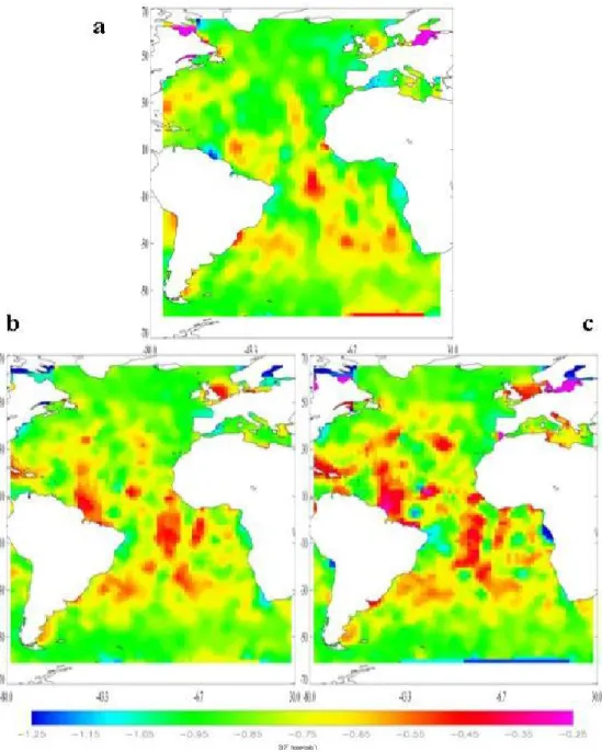
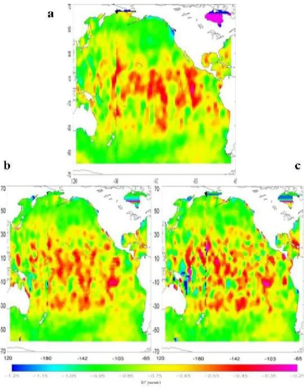
Fig. 3. Geographical distribution of BF in the Atlantic Basin, obtained for the three time samplings considered. (a) 1t = 35 days, (b) 1t = 11 days and (c) 1t = 4 days.

3.1 LRA results

The SLA data will be fitted to the DSP data through the sim-ple linear regression equation:

SLA(8, λ, T ) = BF [DSP (8, λ, T )] + ε (9) where the regression coefficient BF may be understood as a barometric factor, and ε is the residual signal which is inco-herent with the atmospheric pressure forcing. So, if residuals are not correlated with DSP, then BF should be close to the value deduced from the isostatic assumption (GP97, PG99 and MW01).

3.1.1 Atlantic Basin

Figure 2 shows the meridional distribution of BF, consider-ing the three different 1t used, i.e. case (a) 35 days, case (b) 11 days and case (c) 4 days. Initially, we obtained the BF values at each position and then averaged them into latitu-dinal bands of 10◦in width. The averages were assigned to the central latitude of each band. We only considered the BF values lying in the range: (−1.20, −0.20) (cm/mb). We de-cided to adopt this criterion because the percentage of points with a value BF out of this range were lesser than 10%. We observe that, in all cases, the ocean response to atmospheric

Fig. 4. As Fig. 2, in the case of the Indian Basin.

pressure variations is close to the isostatic one at mid and high latitudes. However, in case (a), we observe a different behaviour at low latitudes, not found in cases (b) and (c). In case (a), the ocean response is, in general, still close to the isostatic one along all the latitudes (except in the latitudinal band: −25◦, −35◦), while in cases (b) and (c) strong devia-tions are found, especially in the vicinity of the equator.

Figure 3 plots the regional distribution of BF. The pro-cedure was to consider all the values at geographic points within 1.5◦_{square windows and then to calculate the mean.} The averaged values are then assigned to the centre of each window and represented in the figure as a function of time (cases (a), (b) and (c)). Independent of the time sampling used, the distribution of BF is not homogeneous, but val-ues between 1.05 and 0.80 cm/mb (green colour) are pre-dominant at mid and high latitudes. Nevertheless, there are some specific regions, especially in the South Atlantic Basin, where we observe small deviations from the isostatic sponse (yellow colour) which are more evident when we re-duce 1t. At low latitudes, the ocean response presents higher deviations with strong departures in some zones (red colour). Also, the deviations increase with lesser 1t.

3.1.2 Indian Basin

Figure 4 plots the meridional distribution of BF. Cases (b) and (c) show a similar behaviour to that found in the AB, es-pecially the marked latitudinal dependence of the ocean re-sponse to atmospheric pressure variations. At mid and high latitudes, the BF values indicate a response near to the static one and at low latitudes strong deviations from the

iso-static response are observed. Nevertheless, in case (a), we observe important differences between both basins, mainly at low latitudes. The values obtained in the second basin indi-cate that at these latitudes, the ocean response to atmospheric pressure is far from isostatic.

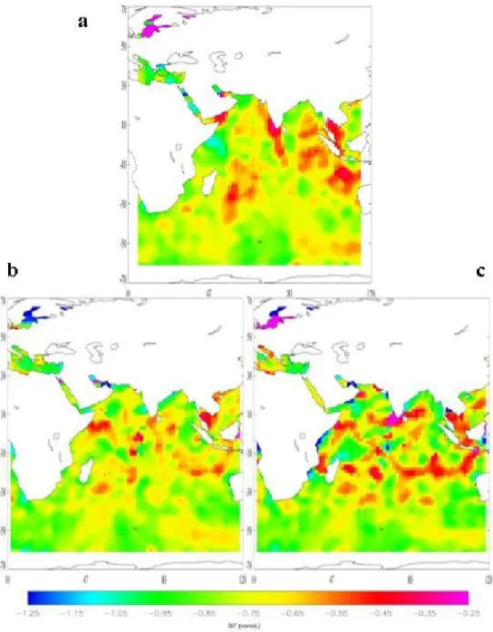
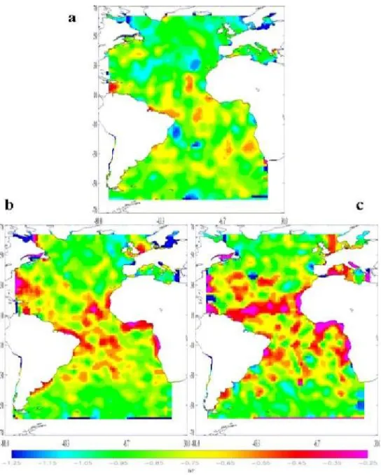
As far as the regional distribution of BF is concerned, Fig. 5 demonstrates that there are three predominant colours in the three cases considered: green, yellow and red. This fact implies that the range of variation of FB oscillates be-tween 1.10 and 0.40 cm/mb. In case (a), the predominant val-ues are between 0.80 and 0.60 cm/mb (yellow colour). Nev-ertheless, we observe some specific zones with values be-tween 0.60 and 0.40 cm/mb (red colour), where the oceanic response is clearly far from isostatic (south of India, Thailand Gulf, south of Indonesia and the east region of Madagascar). Values in the range (1.10, 0.80) cm/mb (green colour) can be found in some regions of the higher latitudes of South Indian Basin. When 1t is reduced (cases (b) and (c)), the value dis-tribution is quite similar in both cases, mainly in the range (1.10, 0.60) cm/mb (yellow and green colours, respectively). There are also some values between 0.60 and 0.40 cm/mb (red colour) in cases (a) and (b), contrary to that observed in the Atlantic Basin.

3.1.3 Pacific Basin

We decided to include in this basin some specific regions, such as the Gulf of Mexico, the Caribbean Sea and Hudson Bay, since they were not included in the analyses performed in the Atlantic Ocean. Because global longitudinal positions vary in the range (180◦_{, −180}◦_{), there is a change of sign in} this basin (horizontal axis in Fig. 7). The longitudinal posi-tions vary in the range (120◦_{, −65}◦_{). Figure 6 demonstrates} that this basin shows the same behaviour as the previous one. At mid and high latitudes, the BF values are quite similar in all cases, indicating an ocean response to pressure forc-ing close to the isostatic case. However, at low latitudes, the ocean response is far from isostatic, even in case (a).

Also, Fig. 7 presents the regional distribution of BF. The reduction in 1t does not excessively modify the magnitude of BF, since the results obtained are very similar in all cases. The values far from the isostatic response (red colours) are found mainly at low latitudes.

3.2 EOFD results

This method consists basically in expressing a given set of simultaneous time series, Si(t ), as a linear combination of a system of orthogonal functions, Pj(t ) named temporal weights (Kundu et al., 1975). Once the latter functions are determined, each one of the time series may be expressed as:

Si(t ) = M

X

j =1

AijPj(t ), (10)

where the subscript i indicates each one of the time series and

J. G´omez-Enri et al.: Different ocean responses to atmospheric pressure variations 337

Fig. 5. As Fig. 3, in the case of the Indian Basin.

fixed i and j = 1, ..., M) are the eigenvector components as-sociated with each one of the eigenvalues of the covariance matrix of the time series. These components are usually des-ignated as spatial coefficients, since they express the relative importance of a given temporal weight in each one of the series with respect to the others. We have to consider the fact that SLA data can be affected by many sources of noise. This circumstance can make it very difficult to find suitable estimations of BF using conventional techniques, such as sin-gle and multiple regression analysis (FP94; Tsimplis, 1995; GP97 and PG99). The EOFD is usually applied to several time series, of values of a single variable, recorded simulta-neously in several spatial locations. However, in the present analysis this technique will be applied on the two different

variables that we are concerning: DSP and SLA, joined in the same EOFD analysis.

The existence of a common temporal weight Pj(t ) be-tween the two variables could characterise a static response of SLA to DSP. Then, the signal corresponding to this tempo-ral weight may be expressed for the variables, respectively, as:

(DSP )ij =ADSPij Pj(t ) (11)

(SLA)ij =ASLAij Pj(t ) (12) where the superscripts of Aij indicate that the spatial coef-ficients are for DSP or SLA. The results obtained with this

Table 2. Global averaged values of BF in the Atlantic Basin (AB), North AtlanticBasin (NAB) and South Atlantic Basin (SAB) estimated

via EOFD and LRA.

1t =35 days 1t =11 days 1t =4 days EOFD LRA EOFD LRA EOFD LRA AB −1.004 −0.850 −0.790 −0.792 −0.725 −0.773 NAB −1.035 −0.877 −0.785 −0.793 −0.654 −0.764 SAB −0.935 −0.821 −0.769 −0.759 −0.760 −0.746

Table 3. Global averaged values of BF in the Atlantic Basin (AB), North Atlantic Basin (NAB) and South Atlantic Basin (SAB).

1t =35 days 1t =11 days 1t =4 days model ERS-2 model ERS-2 model ERS-2 AB −0.862 −0.891 −0.849 −0.852 −0.824 −0.832 NAB −0.864 −0.894 −0.847 −0.852 −0.813 −0.827 SAB −0.852 −0.892 −0.824 −0.829 −0.793 −0.805

Fig. 6. As Fig. 2, in the case of the Pacific Basin.

technique are shown in Fig. 8. The behaviour of the distri-bution of values is quite similar to that estimated with LRA (Fig. 2), in the sense that when we reduce 1t, there are spe-cific areas where the ocean response is far from the isostatic response. The most important deviations are found with

1t =4 days. This fact is more evident at low latitudes. At mid and high latitudes some discrepancies exist between the results obtained in both hemispheres. The results are

practi-cally identical in South Atlantic Basin to those obtained with LRA, whereas in the North Atlantic Basin there are differ-ences which oscillate between 0.20 and 0.30 cm/mb.

It can be noted that the greatest discrepancies between LRA and EOFD are found in case (a). With EOFD the range of variation of BF is a little higher than in the LRA. Anyway, they are within a logical range of variation from the point of view of the ocean response to pressure varia-tions. Differences between both techniques are not higher than 0.30 cm/mb (absolute value), except in the case (a) in the latitudinal band (35◦_{, 25}◦_{). Table 2 compares the global} average of BF values estimated with the two techniques. The results demonstrate that at the global scale there are some divergences, but not higher than 0.10 cm/mb, except in case (a), where we note differences higher than 0.20 cm/mb.

Figure 9 shows the geographical distribution of BF values computed via EOFD. There are great similarities with the BF distribution obtained with LRA in all cases. From this figure we can infer the same behaviours described with LRA. The greatest differences are found in the range of variation of BF values. With EOFD, this is a little wider. Some specific regions have values between 1.15 and 1.05 cm/mb (sky-blue colour), especially at mid and high latitudes of the Northern Atlantic.

3.3 Model results

The inclusion of global barotropic ocean models in the study of the ocean’s response to atmospheric pressure variations is still a recent development. We note some works, especially those of Ponte et al. (1991), PG99, MW01 and GE01.

Figure 10 shows the comparison between the LRA results by using the model and satellite data at the three time sam-plings used. We deduce that the ocean response to

atmo-J. G´omez-Enri et al.: Different ocean responses to atmospheric pressure variations 339

Fig. 7. As Fig. 3, in the case of the Pacific Basin.

spheric pressure variations is similar in the two data sets, since in the three cases, practically the same meridional vari-ation is observed. As far as the influence of 1t in the merid-ional distribution of BF is concerned, it can be noted that the ocean response is further from the isostatic case when 1t is less only in the latitudinal bands close to the equator. Never-theless, the response is practically isostatic in case (a) at all latitudinal bands.

Table 3 summarises the global averaged values of BF ob-tained with model results and satellite data. We simply esti-mated the global mean from the complete set of values that we obtained at each geographic location. Differences ob-served between both data sets are not too important, inde-pendent of the 1t used (not higher than 0.05 cm/mb).

Shown in Fig. 11 is the comparison between the re-gional distribution of the BF values, considering the model (Figs. 9a, 9c, and 9e) and the altimeter records Figs. 9b, 9d

Fig. 8. Meridional distribution of BF estimated using EOFD

tech-nique at different time samplings: 35 days (gross solid line), 11 days (thin solid line) and 4 days (dashed line).

and 9f). Distributions are quite similar between them. The greatest differences are found at 1t = 4 days, because in the case of the model results, the values between 0.60 and 0.40 cm/mb (red colour) are concentrated in a thin band close to the equator, whereas in the case of satellite records, such range is more disperse at low latitudes.

4 Discussion

The linear regression analysis in the three basins demon-strates that at mid and high latitudes, the ocean responds to the atmospheric pressure variations in a similar manner to that deduced from the Isostatic Assumption, with BF close to 0.995 cm/mb. However, at lower latitudes, this response is far from isostatic, with deviations that reach 50% of the the-oretical value. This behaviour is not dependent on the time sampling used (35, 11 or 4 days), with the exception of the Atlantic Basin, where in the case of 1t = 35 days, the ocean response is close to the isostatic one, in the equatorial regions as well. In the next section we will try to clarify the reasons for this fact.

Following GP97, PG99 and MW01, the decrease in the BF values in the tropical and equatorial bands may be basically explained in terms of the non-inverted-barometer response (dinamical response) of the sea level to the atmospheric pres-sure forcing. On the other hand, the main reason to explain the dependence on the 1t of the BF estimates could lie in the fact that while is smaller the 1t, a higher frequency of the signal is stressed. At the same time, since the departures

from the IB response are greater for the higher frequencies, the BF estimates corresponding to a smaller 1t will devi-ate more from the IB response than those corresponding to a greater 1t .

GP97, on the basis of TOPEX-Poseidon data, found ev-idence for this by dependence comparing the BF estimates using crossover differences (1t = 4 days) with those ob-tained using co-linear differences (1t = 10 days). However, PG99 using the same set of TOPEX-Poseidon data showed that when the crossover analysis of GP97 is repeated, tak-ing into account the diurnal and semidiurnal atmospheric tide signals contained in the atmospheric pressure series, the BF produced values are significantly higher than those obtained in GP97. In this way, if we consider the results of PG99, the differences between crossover and co-linear BF values is notably attenuated with respect to the GP97 results and the dependence of the BF estimates on 1t is not so evident.

To this respect, it is convenient to point out that the repeat-ing cycle period of the ERS-2 satellite record data (35 days) is not affected by the aliasing produced by the atmospheric tide signal. Our BF estimates show little difference between the analysis results corresponding to 1t = 4 and 11 days, which is in accordance with the PG99 result.

In the Atlantic basin, the BF estimated via EOFD show similar results to those obtained with LRA. It can also be ob-served that at mid and high latitudes, the ocean response is still close to the isostatic case, whereas in equatorial regions there are important discrepancies with respect to the theoret-ical value, mainly for 1t = 11 and 4 days. This technique is an alternative to the classical linear regression analysis, which is normally used in satellite altimetry studies to esti-mate the barometric factor. Moreover, it provides the ability to contrast the results obtained with the LRA technique, es-pecially in those zones where the statistical confidence level is especially low (tropical and equatorial regions). The BF estimates made via EOFD analysis produced a similar result regarding as to their dependence on the 1t used. The ab-solute values of the BF are greater for 1t = 35 days. This analysis provides an independent result that supports the de-pendence on 1t found with the LRA technique.

Regarding the numerical model results, these are in good agreement with the altimeter data results. The decrease in the BF estimates through the tropical and equatorial bands is quite similar to that shown in the altimeter data analysis and there is also a clear dependence of these estimates on the 1t used. The BF absolute value for 1t=35 days is significantly higher than those found in the 1t = 4 and 11 day cases. There is little difference between the values corresponding to the latter cases. All these characteristics are found in the altimeter data analysis. The consistency between model and observed data estimates help in building confidence in the data quality of the ERS altimeter.

The agreement between the numerical model and altimer data results allow us to infer that the main factors used to ex-plain the spatial variations of BF estimates must be related to the sea level response to atmospheric pressure and wind, the only forcing variables in the numerical model.

There-J. G´omez-Enri et al.: Different ocean responses to atmospheric pressure variations 341

Fig. 9. Geographical distribution of BF in the Atlantic Basin, obtained via EOFD for the three time samplings considered. (a) 1t = 35 days, (b) 1t = 11 days and (c) 1t = 4 days.

fore, other causes of sea level variation in the tropical and equatorial bands as the steric effects associated with non-propagating seasonal variations or the existence of baroclinic Rossby and Kelvin waves, seem to have little importance in explaining the spatial variations of the BF estimates. This conclusion is in accordance with Polito and Liu (2003), who showed, on the basis of TOPEX-Poseidon data, that in the Atlantic basin neither non-propagating seasonal variations nor planetary (Rossby, Kelvin and instability) waves are so important in the explanation of the sea level variance as they are in the Indian and Pacific Basins.

On the basis of the previous discussion, we conclude that in the Atlantic Basin the variation of the BF estimates through the tropical and equatorial bands may be basically

explained, in accordance with PG99, in terms of the non-inverted-barometer response (dinamical response) of the sea level to the atmospheric pressure forcing in the equator. The higher absolute values of BF found in the case 1t = 35 days in the tropical and equatorial bands may be due to the fact that the stressed signal in this case, that of a period around 70 days, shows a response to the atmospheric pressure varia-tions closer to the theoretical isostatic one. The detection of this response via LRA or EOFD techniques has been likely aided by the little relative importance that seasonal oscil-lations have in the tropical and equatorial Atlantic. Since GP97, PG99 and MW01 did not use 1t = 35 days, it is im-possible to know if this same result would have been found with TOPEX-Poseidon data.

Fig. 10. Comparative between the meridional distribution of BF estimated using ERS-2 records (thin solid line) and the outputs of

the Barotropic Ocean Model (gross solid line), considering the three time sampling used. (a) 1t = 35 days, (b) 1t = 11 days and

(c) 1t = 4 days.

In the Indian and Pacific Basins the absolute values of the BF estimates show a similar decrease with latitude for the three different 1t used. Unlike the Atlantic Basin in the In-dian and Pacific Oceans, the sea level signal associated with the steric effects of seasonal periods and with baroclinic plan-etary waves represents an important part of the total signal (Polito and Liu, 2003). The seasonal variations have a pe-riod of around 90 days and they can be due to steric effects or baroclinic planetary waves. The planetary waves may have periods greater than the seasonal one, but also greater than the intraseasonal periods as well. Enfield (1987) and McPhaden and Taft (1988) have documented sea level prop-agating fluctuations of 40–90 days across the equatorial Pa-cific. Regarding the Indian Basin, Sengupta et al. (2001) have recorded current velocity oscillation of 20–60 day periods in

the western Indian Ocean which seem to be related to baro-clinic planetary waves.

In the presence of the above commented signals, either EOFD or LRA techniques could find false IB-like sea level responses to seasonal variations of the atmospheric pressure when the former signals are in phase or anti-phase with re-spect to the latter. In the case of CT differences with a

1t = 35 days, the signal stressed is that having a period of 70 days. Therefore, if a seasonal or intraseasonal (of pe-riod around 70 days) signal is present in the sea level record, the CT differences will reinforce them against other signals with periods far away from 70 days, that is, signals with peri-ods close to 70 days are amplified in the CT sequences while signals with periods far from 70 days are diminished.

J. G´omez-Enri et al.: Different ocean responses to atmospheric pressure variations 343

Fig. 11. Comparative between the geographical distribution of BF estimated from the ERS-2 data; (a) 1t = 35 days, (c) 1t = 11 days and (d) 1t = 35 days and the outputs from the barotropic ocean model; (b) 1t = 35 days, (e) 1t = 11 days and (f) 1t = 35 days.

As previously commented, in our analysis on the Indian and Pacific Basins we did not find significatively different BF estimates along the tropical and equatorial bands in the case when 1t = 35 days with respect to those obtained for

1t = 4 and 11 days. We think that the reason for that a higher absolute value of BF has not been found in the case of

1t =35 days may lie in the interaction between the isostatic sea level response and these seasonal and intraseasonal sig-nals, which are of great relative importance in these basins. Such a response may be existing but it may not be sepa-rated from the seasonal or intraseasonal signals which may show incidental correlations with atmospheric pressure vari-ations. It is of crucial importance to inquire whether or not in these basins a closer to isostatic sea level response for pe-riods around 70 days or greater exists, in order to correctly apply the inverse barometer correction on the altimetric data. Otherwise, after the correction is applied, a considerable part of the isostatic sea level response (say that explained by near seasonal periods) may remain in the sea level and be inter-preted as a false seasonal signal in subsequent analysis.

Acknowledgements. This work has been developed at the Applied

Physics Department (University of C´adiz- Spain) and ESRIN (Eu-ropean Space Agency-Italy) and it was funded partially by the Span-ish Education Department. The authors want to thank J. Benveniste for his support and advices. We would also like to thank V. Zlot-nicki and A. Haide Ali from the Jet Propulsion Laboratory, who provided the barotropic model outputs and J. R. Mason, Science and Technology Officer from the Naval European Meteorology and Oceanography Center in Rota (Spain), for his review of the English. Topical Editor N. Pinardi thanks two referees for their help in evaluating this paper.

References

Benveniste, J.: Minutes of the ERS-2 Radar Altimeter and Mi-crowave Radiometer Commissioning Working Group (#9), ESA-ESRIN 30.–31.1.1996, rs/pm/jb/96.009, ESA-ESRIN, Frascati, 1996a. Benveniste, J.: Minutes of the ERS-2 Radar Altimeter and Mi-crowave Radiometer Commissioning Working Group (#10), ESA-ESRIN 25.–26.4.1996, rs/pm/jb/96.026, ESRIN, Frascati, 1996b.

Centre ERS d’Archivage et de Traitment (CERSAT) and ESA Al-timeter and microwave radiometer ERS products, user manual (version 2.2), Plouzan´e, France, 1996.

Cheney, R. E., Marsh, J. G., and Beckley, B. D.: Global Mesoscale Variability from Collinear Tracks of SEASAT Altimeter Data, J. Geophys. Res, V. 88, 4343–4354, 1983.

Close, C.: The fluctuations of mean sea-level with special reference to those caused by variations in barometric pressure, Geographi-cal Journal, 52, 51–58, 1918.

Dorandeu, J. and Stum, J.: CLS contribution to the ERS-2 radar al-timeter range bias determination using OPR2, ERS-2 RA/MWR Commissioning Working Group final report, ESA contract no. 143187 from 15/09/1994, Available from ESA/ESRIN, 17 pp, 1996.

Enfield, D.: The intraseasonal oscillation in eastern Pacific sea lev-els: how is it forced?, J. Phys. Oceanogr., 17, 1860–1876, 1987.

Fu, L.-L. and Pihos, G.: Determining the response of sea level to atmospheric pressure forcing using TOPEX/POSEIDON data, J. Geophys. Res., 99, 24 633–24 642, 1994.

Gaspar, P. and Ogor, F.: Estimation and analysis of the sea state bias of the new ERS-1 and ERS-2 altimetric data, Report of task 2 of IFREMER contract n. 96/2.246 002/C, 1996.

Gaspar, P. and Ponte, R. M.: Relation between sea level and baro-metric pressure determined from altimeter data and model simu-lations, J. Geophys. Res., 102, 961–71, 1997.

Gaspar, P. and Ponte, R. M.: Correction to “Relation between sea level and barometric pressure determined from altimeter data and model simulations”, J. Geophys. Res., 103, 18 809, 1998. Gill, A. E.: Atmosphere-Ocean Dynamics, Academic Press, 662

pp., 1982.

Gill, A. E. and Niiler, P. P.: The theory of the seasonal variability in the ocean, Deep-Sea Res., 20, 141–177, 1973.

Gissler, N.: Anledning at finna Hafvets affall f¨or vissa ar, in Kungliga Svenska Vetenskapsakademiens Handlingar, 142–149, Stockholm, 1747.

G´omez-Enri, J., Villares, P., Bruno, M., and Benveniste, J.: Estima-tion of the Atlantic sea level response to atmospheric pressure us-ing ERS-2 altimeter data and a Global Ocean Model, in: SPIE In-ternational Symposium on Remote Sensing. ISBN 0-8194-4269-0, 2001.

Hirose, N., Fukumori, I., Zlotnicki, V., and Ponte, R. M.: High-Frequency Barotropic Response to Atmospheric Disturbances: Sensitivity to Forcing, Topography, and Friction, J. Geophys. Res., 106, 30 987–30 996, 2001.

Kundu, P. K., Allen, J. S., and Smith, R. L.: Modal Decomposition of the Velocity Field near the Oregon Coast, J. of Phys. Oceanog-raphy, 3, 683–704, 1975.

Loial, C.: USO and SPTR correction files, Minutes of the ERS-2 Radar Altimeter and Microwave Radiometer Commissioning Working Group (#9), ESA-ESRIN, 1996.

Lubbock, J. W.: On the tides at the port of London. Philosophi-cal Transactions of the Royal Society of London, 126, 217–266, 1836.

Mathers, E. L. and Woodworth, P. L.: Departures from the local inverse barometer model observed in altimeter and tide gauge data and in a global barotropic numerical model, J. Geophy. Res., 106, 6957–6972, 2001.

McPhaden, M. J. and Taft, B. A.: Dynamics of seasonal and in-traseasonal variability in the eastern equatorial Pacific, J. of Phys Oceanogr., 18(11), 1713–1732, 1988.

Polito, P. S. and Liu, W. T.: Global characterization of Rossby waves at several spectral bands. J. Geophys. Res., 108, 3018, doi: 10.1029/2000JC000607, 2003.

Ponte, R. M., Salstein, D. A., and Rosen, R. D.: Sea level response to pressure forcing in a barotropic numerical model, J. Phys. Oceanogr., 21, 1043–1057, 1991.

Ponte, R. M.: Variability in a homogeneous global ocean forced by barometric pressure, Dyn. Atmos. Oceans, 18, 209–234, 1993. Ponte, R. M.: Understanding the relation between wind- and

pressure-driven sea level variability, J. Geophys. Res., 99, 8033– 8039, 1994.

Ponte, R. M. and Gaspar, P.: Regional analysis of the inverted barometer effect over the global ocean using TOPEX/POSEIDON data and model results. dJ. Geophys. Res., 104, 15 587-15 601, 1999.

Roden, G. I.: Low-frequency sea level oscillations along the Pacific coast of North America, J. Geophys. Res., 71, 4755–4776, 1966. Ross, J. C.: On the effect of the pressure of the atmosphere on the

J. G´omez-Enri et al.: Different ocean responses to atmospheric pressure variations 345 mean level of the ocean. Philosophical Transactions of the Royal

Society of London, 144, 285–296, 1854.

Rossiter, J. R.: Long-term variations in sea-level, The Sea, vol. 1, edited by Hill, M. N., Wiley-Interscience, New York, 590– 610, 1962.

Saastamoinen, J.: Atmospheric correction for the troposphere and stratosphere in radio ranging of satellites, Geophys. Monogr., 15, AGU, Washington, D.C., 1972.

Scharroo, R. and Visser, P. N. A. M.: Precise orbit determination and gravity field improvement for the ERS satellites, J. Geophys. Res., 103, 8113–8127, 1998.

Sengupta, D., Senan, R., and Goswani, B. N.: Origin of intrasea-sonal variability of circulation in the tropical central Indian Ocean, Geophysical Research Letters, 28(7), 1267–1270, 2001. Tsimplis, M. N.: The response of sea level to atmospheric forcing in

the Mediterranean, J. of Coastal Res., 11 (4), 1309–1321, 1995. van Dam, T. M. and Wahr, J.: The atmospheric load response of the

ocean determined using Geosat altimeter data, Geophys. J. Int., 113, 1–16, 1993.

Wunsch, C. and Stammer, D.: Atmospheric loading and the oceanic “inverted barometer” effect, Reviews of Geophysics, 35, 79–107, 1997.