Diagnosing and Mitigating Market Power in Chile's Electricity Industry by 03-010 May 2003 M. Soledad Arellano WP
Diagnosing and Mitigating Market Power in Chile’s
Electricity Industry.
∗
M.Soledad Arellano
†Universidad de Chile
May 12, 2003
AbstractThis paper examines the incentives to exercise market power that generators would face and the different strategies that they would follow if all electricity supplies in Chile were traded in an hourly-unregulated spot market. The industry is modeled as a Cournot duopoly with a competitive fringe; particular care is given to the hydro scheduling decision. Quantitative simulations of the strategic behavior of generators indicate that the largest generator (”Endesa”) would have the incentive and ability to exercise market power unilaterally. It would do so by scheduling its hydro resources, which are shown to be the real source of its market power, in order to take advantage of differences in price elasticity: too little supply to high demand periods and too much to low demand periods. The following market power mitigation measures are also analyzed: (a) requiring Endesa to divest some of its generating capacity to create more competitors and (b) requiring the dominant generators to enter into fixed price forward contracts for power covering a large share of their generating capacity. Splitting the largest producer in two or more smaller firms turns the market equilibrium closer to the competitive equilibrium as divested plants are more intensely used. Contracting practices proved to be an effective tool to prevent large producers from exercising market power in the spot market. In addition, a more efficient hydro scheduling resulted. Conditions for the development of a voluntary contract market are analyzed, as it is not practical to rely permanently on vesting contracts imposed for the transition period.
JEL Codes: D43, L11, L13, L94
Key Words: Electric Utilities; Market Power; Scheduling of Hydro-Reservoirs; Contracts; Chile’s Electricity Industry
∗I am grateful to Paul Joskow and Franklin Fisher for their comments and suggestions. I also benefited from
comments made by participants at the IO lunches and the IO Seminar held at MIT and from Seminars held at the Instituto de Economia, Universidad Católica de Chile and Centro de Economía Aplicada, Universidad de Chile. Financial support from the MIT Center for Energy and Environmental Policy Research (CEEPR) is gratefully acknowledged.
†Center of Applied Economics, Department of Industrial Engeneering, Universidad de Chile. República
1
Introduction
Chile reformed and restructured its power industry in the early 1980’s. Competition among generators was promoted and a ’simulated’ spot market was created. Prices in this market were not truly deregulated (except for the largest consumers who chose to enter into contracts directly with generators) but were based in the short-run marginal costs of generators in the system and the associated least cost dispatch. Two decades later, policymakers in Chile are discussing the desirability of further de-regulating Chile’s wholesale electricity market. In particular, the simulated spot market that is in place today would be replaced by a real un-regulated spot market in which generators would be free to bid whatever prices they choose with competition between generators determining the bids and market clearing prices. One major concern that has been raised regarding this spot market deregulation proposal is that the high degree of concentration in the generation segment would enable incumbent gener-ators to exercise market power, leading to prices far above competitive levels. International experience on restructuring and reforms of the electricity industry on different countries (UK, US, New Zealand and so on) has taught us that this concern is legitimate. First of all, poli-cymakers must realize that the electricity industry is prone to the exercise of market power, as electricity cannot be stored, demand is very inelastic, producers interact very frequently, capacity constraints may be binding when demand is high and thus even a small supplier may be able to profitably and unilaterally increase the market price by withholding supplies from the market. The importance of an adequate number of generating companies that compete in the wholesale market has also been emphasized. For instance, the experience in the UK, has shed light on the market power problems that high concentration may create and dur-ing the late 1990s, the government embarked on a program to reduce concentration through divestiture and the encouragement of competitive entry. 1
This paper examines the incentives to exercise market power that generators would face and the different strategies that they would follow if all electricity supplies in Chile were traded in an hourly-unregulated spot market. The analysis will focus on the impact of such a reform in the biggest Chilean electric system, called the ”SIC”. Its installed capacity amounts to 6660 MW. Electricity is produced by 20 different generating companies but two economic groups (called Endesa and Gener) control 76% of total installed capacity and 71% of total generation. These firms differ in size, composition of its production portfolio and associated marginal cost functions. Endesa (”Firm 1”) owns a mixed hydro/thermal portfolio, concentrates 78% of the systems’ hydro reservoir capacity and its thermal capacity covers a wide range of fuel and efficiency levels. Gener (”Firm 2”) is basically a purely thermal producer and concentrates the largest fraction of thermal resources in the SIC (46%). Analyzing Chile’s sector is especially interesting because a large fraction of its generating capacity is stored hydro. Previous analyses have focused on systems that were either mostly thermal or entirely hydro (e.g. Norway).
Following Borenstein and Bushnell (1999) and Bushnell (1998), Chile’s electricity market is modeled as a Cournot duopoly with a competitive fringe. Particular care is given to the modeling of hydro resources, which are not only important because of its large share in total installed capacity and in total generation (61% and 62% respectively in 2000), but because of its impact on the incentives faced by producers when competing. As it will be analyzed in
the paper, having hydro resources as a source of electric generation, means that firms do not take static production decisions at each moment in time, but that firms have to take account that more water used today, means less water is available for tomorrow: the model becomes dynamic rather than static.
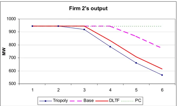
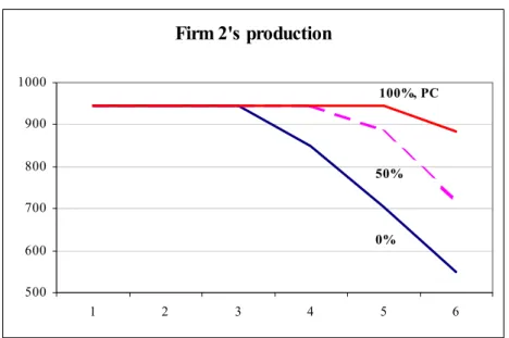
Quantitative simulation results suggest that if an unregulated spot market were imple-mented in Chile, prices could rise far above competitive levels as suppliers, in particular Endesa, the largest supplier, would exercise unilateral market power. The large thermal portfolio owned by Gener, the second largest generator, is not enough for the exercise of mar-ket power, as the relevant plants are mostly base load plants. Indeed, Endesa has so much market power and can move prices up so much, that Gener’s optimal strategy is to produce at full capacity, profiting from the high prices set by Endesa. Even though Endesa keeps most of its thermal plants outside of the market, the real source of its market power is its large hydro capacity. In particular, it schedules its hydro production in order to exploit differences in price elasticity, allocating too little supply to high demand periods and too much to low demand periods, relative to the competitive equilibrium. This hydro scheduling strategy may be observed no matter what planning horizon is assumed in the model (a month, a year); the only ”requirement” is that there is enough ”inter-period” differences in demand elastic-ity. The smaller are the intertemporal differences in demand elasticities, the closer is the hydro scheduling strategy to the traditional competitive supply-demand or value-maximizing optimization analysis’ conclusions (i.e. water is stored when it is relatively abundant and released when it is relatively scarce). The importance of hydro resources for Endesa is such that when hydro flows are reduced (as occurs if the hydrological year is ”dry”), Endesa loses its market power. Under these circumstances, Gener has incentives to act strategically to increase prices, but the resulting prices are still lower than when Endesa had all of its capacity under normal hydrological conditions. Not surprisingly, alternative assumptions about the elasticity of demand for electricity turned out to be very important, as the more elastic is demand, the less market power can be exercised.
These results suggest that the exercise of market power should be of considerable con-cern in Chile and that mitigation measures will be needed to prevent market power abuses in the newly deregulated spot market. Different market rules have been implemented as a shield against market power abuses throughout the world. Regulators have relied on elements such as splitting the generating companies into many small firms in order to reduce the de-gree of concentration of the generation sector (Australia, Argentina), vesting contracts in order to reduce generating companies’ incentives to charge high prices (England and Wales, Australia) and continuing regulatory surveillance and threats (England and Wales, United States), among others. Each country / electric power system is different in terms of market structure, size, mix of generating technology and even culture. As a consequence, the experi-ence of another market, even if successful, should not blindly be put into practice elsewhere without first carefully analyzing the individual characteristics of the specific electric power industry subject to reform. The effect of different market power mitigation measures that have been implemented in other restructured electricity markets are also thoroughly analyzed in this paper for the case of Chile’s electricity industry. In particular, I analyze and estimate the impact of two different sets of measures that could be implemented to reduce the incen-tive and ability of the dominant firms to exercise market power in a spot wholesale electricity market in Chile: (a) requiring the largest firm to divest some of its generating assets and (b) requiring the largest firms to enter into fixed price forward contracts covering a large share
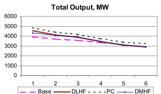
of their capacity. I compare the new market equilibrium to the competitive equilibrium and to the base model equilibrium, in terms of aggregate levels, allocation of resources, markups and overall welfare (when possible).
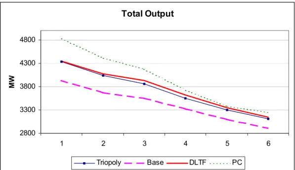
The divestiture of some of Firm 1’s generating assets, either thermal or hydro storage plants, turns the market equilibrium closer to the competitive equilibrium not only in terms of levels (prices and output) but also in terms of the allocation of resources, as former Firm 1’s plants are more intensely and efficiently used and this more than compensates for any reduction in production by the remaining producers with unilateral market power. The application of fixed price forward contracts proved to be an effective tool to prevent large producers from exercising market power in the spot market. In addition, a more efficient hydro scheduling resulted. It is argued that it is not practical to rely permanently on vesting contracts to ensure the development of the contract market as these contracts will eventually expire and if conditions are not given for an appropriate voluntary contracting, market power abusive practices will certainly take place at that time. It is emphasized that the regulation of the industry as a whole (as opposed to the contract market) must provide the incentives for producers and consumers to contract.
This paper is organized as follows: the next chapter reviews the main findings of the literature that are related to the topics covered in the paper. In Chapter 3 I briefly describe the Chilean power industry. In the fourth Chapter I analyze the model that will be the basic tool for the analysis of market power in Chile’s electricity industry. Data used to estimate the model are reported in Chapter 5. Quantitative simulations of each generators’ strategy and the resulting market equilibrium are estimated under different assumptions in Chapter 6. In Chapter 7, a modified version of the basic model is used to estimate the impact of two sets of mitigation measures. Both a qualitative and a quantitative analysis are done. Chapter 8 concludes.
2
Literature Review
This paper is related to three areas of research: the modeling of electricity markets in order to (ex-ante) simulate strategic behavior after the industry has been deregulated, the analysis of the strategic use of hydro resources to exercise market power and the impact of forward contracting on the incentives producers face to exercise market power.
Three types of model have been used to simulate the strategic behavior of electricity firms. In the supply function equilibrium (SFE) approach, used by Green and Newbery (1992) and Halseth (1998) based on the work by Klemperer and Meyer (1989), the producers bid a supply function that relates quantity supplied to the market price. In the general case, the duopoly supply lies between the competitive and Cournot equilibrium; the range of feasible equilibria is reduced when uncertainty is added to the model.
Green and Newbery (1992) modeled the England and Wales electricity market using the Supply Function Equilibrium (SFE) framework developed by Klemperer and Meyer (1989) as applied to an empirical characterization of supply and demand, designed to match the attributes of the electricity system in England and Wales (making alternative assumptions about the elasticity of demand).2 They first present simulated values for prices, output 2Von der Fehr and Harbord (1993) and Halseth (1998) criticize on theoretical grounds the Green and
and welfare for the duopoly case. They found that generators were able to drive prices far above competitive levels, depending on the assumed elasticity of demand, while creating a significant deadweight loss and producing supra-competitive profits for the generators.3 They
then examined the impact of restructuring the industry so that there were five equal-sized firms. In this case, the equilibrium price was significantly lower and close to competitive levels. In order to take account of the effect of potential entry, they examined the effects of entry in the duopoly case under alternative assumptions about the price responses of the incumbents to the entry of generators who acted as price takers. If the incumbents adopted a strategy of not responding to entry by lowering prices, substantial entry was attracted by the excess profits in the system. Eventually entry eroded the incumbents’ profits completely, yielding an equilibrium with inefficient expenditures on new generating capacity and high prices. The welfare losses in these cases were very large.
Halseth (1998) used the SFE approach to analyze the potential for market power in the Nordic market. In his model, the supply function is restricted to be linear, with a constant markup over marginal cost. This markup is independent of the particular technology used by the producer but it varies between the different time periods. Asymmetry in production technologies is incorporated through the marginal cost function (each production level is as-sociated to a specific marginal technology (hydro, nuclear or thermal). Due to the importance of hydro production in the Nordic market (it accounts for 50% of annual production), the hydro scheduling issue is explicitly modeled. In particular, annual hydro production is re-stricted to be less than the annual inflow and the water inflow that is stored between periods has to be within the reservoir capacity. He found that the potential for market power was less than expected due to the fringe’s excess capacity. Only two of the six largest producers had incentives to reduce production.4 Remaining producers did not have incentive to do so. In
particular, he found that hydro producers were not interested in reducing its market supply. He argued that since all of its income came from hydro production (with a very low marginal cost), the price increase had to be very large in order to induce it not to use its generating capacity to the full.5 It should be noted that all the results of this model are reported in
annual terms. In particular, he found that hydro generating capacity was used to the full in the year. However, nothing is said regarding how it is allocated throughout the year. This is an important omission because it may be the case that hydro producers do not exercise market power by using less than its hydro capacity but through a strategy that distinguishes between periods of high demand from periods of low demand.
Auction theory has also been used to analyze strategic behavior in the electricity market. Von der Fehr and Harbord (1993) model the UK electricity spot market as a first price, sealed-bid, multiple unit private-value auction with a random number of units. In their model, generators simultaneously bid supply schedules (reflecting different prices for each individual plant), then demand is realized and the market price is given by the offer price of the marginal plant. They argue that producers face two opposing forces when bidding: by bidding a high price, the producer gets higher revenue but a lower probability of being dispatched.
3Wolfram (1999) found that prices in the British market had been much lower than what Green and
Newbery (1992) predicted.
4These two producers are Vattenfall and IVO. The portfolio of the first one is split between hydro (42%),
nuclear (48%) and conventional thermal plants (10%). IVO is mostly a thermal producer.
5Johnsen et al (1999) concluded from this result that market power cannot be exercised in a market
Equilibrium has different properties depending on the demand level. In particular, when demand is low, producers bid a price equal to the marginal cost of the least efficient generator and equilibrium is unique. When demand is high, there are multiple equilibria and the price is equal to the highest admissible price.6 They remark that some of these equilibria may
result in inefficient dispatching: the high cost generator will be dispatched with its total capacity if it submitted the lowest bid, while the low cost generator will be dispatched for only a fraction of it. Finally they argue that their model is supported by the bidding behavior observed in the UK electricity industry from May 1990 to April 1991. In particular, they report that while bids were close to generation cost at the beginning of the period, they diverged thereafter, Even though contracts were in place in the first part of the analyzed period, they argue that contracting practice is not a plausible explanation to the observed bidding behavior because contracts started to expire after the change of pattern took place. The coincidence of the first period with the low demand season (warm weather) and the second with the high demand season (cold weather) makes their model a more appropriate explanation. It should be noticed however that they analyzed a very short period. In order to be really able to separate the contract effect from the high/low demand effect, and in this way to get more conclusive support to their theory, the following seasons should be analyzed.7
Finally a third approach that has been used in the literature is to model the electricity industry as a Cournot oligopoly where producers are assumed to bid fix quantities. An-dersson and Bergman (1995) simulated market behavior of the Swedish electricity industry after deregulation took place. They assumed a constant elasticity demand function (with an elasticity of demand equal to 0.3 in the main case), constant marginal costs for hydro and nuclear power plants and a non-linear marginal cost function for conventional thermal units. They found that prices would increase and production would be constrained. In particular, they found that the Cournot price equilibrium was 36% higher than the current (base) case and 62% than the Bertrand equilibrium. Markups were not analyzed. They also analyzed the impact of alternative market structures like splitting the largest company in 2 firms of the same size and a merge between the six smallest companies. In both cases equilibrium price was reduced below the base case. Finally they analyzed the impact of increased price responsiveness solving the model for a higher elasticity value (0.6). Since hydro production is modeled on an average basis, nothing is said regarding how resources are allocated within the year (for instance there is no differentiation between peak and off peak periods). In addition, nothing is said regarding how the portfolio of resources is used and how it compares to the base and Bertrand equilibrium cases. This is an important omission given the importance of hydro resources in the Swedish electricity market.
Borenstein and Bushnell (1999) and Bushnell (1998) modeled the California power in-dustry as a Cournot triopoly with a competitive fringe.8 Cournot producers face a residual
demand where must run generation, the fringe’s supply and hydro generation in the case of Borenstein and Bushnell (1999) are subtracted from total demand. Marginal cost functions were estimated using cost data at the plant level. A big difference between those articles is given by the treatment of hydro resources: Bushnell (1998) assumes that Cournot producers
6Multiplicity of equilibria is given by the fact that both producers want to be the ”low bidder” because
the received price is the same but the producer is ranked first, and thus output is greater.
7Wolfram (1998) analyzes the bidding behavior in the UK and tests the theoretical predictions of the multi
unit auction theory.
use them strategically while Borenstein and Bushnell (1999) assume that they are allocated competitively.9 In other words, in Bushnell (1998)’s model, hydro producers are ”allowed”
to store water inflows from one period and use them in another one in order to manipulate prices. As a result, in his model the different periods are not independent and thus the maximization has to be solved simultaneously over the entire planning horizon, as opposed to Borenstein and Bushnell (1999)’s model where each period can be treated independently. Borenstein and Bushnell (1999) use a constant elasticity demand and estimate the model for a range of demand elasticity values (-0.1, -0.4 and -1.0) and six different demand levels. They found that the potential for market power was greater when demand was high and the fringe’s capacity was exhausted, making it impossible for the small producers to increase production. In lower demand hours, Cournot producers had less incentive to withhold production because the fringe had excess capacity. In addition they found that the more elastic was demand, the less was the incentive to exercise market power. Finally they analyzed the hydro scheduling issue by allocating hydro production across periods so as to equalize marginal revenue. They found that even though the resulting hydro allocation was very different from the one implied by the peak shaving approach, prices did not change much because as hydro production was moved out from one period, the resulting price increase induces the other large producers and the fringe to increase production. This result is different from Bushnell (1998)’s findings.
Overall, the literature seems to agree on the following conclusions: more market power can be exercised when the fringe’s capacity is exhausted (which usually occurs when demand is high) because this makes the residual demand curve faced by the firms with market power less elastic. The exercise of market power results in high prices, reduced output and in an inefficient allocation (production costs are not minimized). Results are very sensitive to the elasticity of demand as well as the elasticity of fringe supply. In order to say something regarding the role of hydro resources in the exercise of market power, a formal study of the hydro scheduling issue is needed.
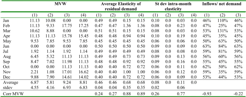
The analysis of the hydro scheduling issue is always done following a similar approach: producers maximize their inter-temporal profits subject to certain constraints such as hydro generation being within a range determined by min and max flow constraints and by the availability of water. Then, an assumption is made regarding what sort of strategy producers may choose. Scott and Read (1996), Scott (1998) and Bushnell (1998) used a quantity strategy and the industry was modeled as a Cournot oligopoly. The main difference between their approaches is given by the method they chose to solve the optimization problem. While Scott and Read used a dual dynamic programming methodology (DDP), Bushnell solved the model by searching for the dual variables that satisfied the equilibrium conditions of the model. In particular, Scott and Read used DDP to optimize reservoir management for the New Zealand electricity market over a medium term planning horizon (1 year). They estimate a ”water value surface” (WVS) that relates the optimal storage level at each period to the marginal value of water (MVW). The latter is interpreted as the marginal cost of generating at the hydro stations. The schedule of the system is determined by running each period a Cournot model in which the hydro plant is treated as a thermal plant using the WVS to determine the marginal cost of water (i.e. MVW), given the period and the storage level at that period.10 The Scott and Read approach is rich in details as hydro
9In particular, hydro production is allocated over the period using a peak shaving technique.
allocation for the whole planning horizon is derived as a function of the MVW. However it is computationally intensive, especially when there is more than one producer who owns hydro-storage plants. It is also data demanding as information on water inflows is required on a very frequent basis. Bushnell modeled the Western US electricity market, where the three largest producers had hydro-storage plants. He adopted a dual method to solve the model, treating the marginal value of water multiplier and the shadow prices on the flow constraints as the decision variables. He derived an analytic solution by searching for values of the dual variables that satisfy the equilibrium conditions at every stage of the multi-period problem. In order to solve his model, he simplified it by assuming that demand and the marginal cost functions were linear.11 The planning horizon was assumed to be one month and the model
was estimated for March, June and September. Bushnell (1998) found that firms could profit from shifting production from peak to off peak hours, i.e. from hours when the fringe was capacity constrained to when it was not. In particular, he estimated that hydro production was reduced by 10% (relative to perfect competition) during the peak hours, resulting in more than 100% price increase. Based on the estimated marginal water values for different months, he found that against what it was expected producers did not shift production from months of high demand to months of low demand. He argued ”since the market is relatively competitive at least some of the time in each month, strategic firms do not need to reallocate across months in order to find hours in which extra output will have little impact on prices”.12
The economic literature, both theoretical and empirical, also shows that the more of a generator’s capacity is contracted forward at fixed prices, the less market power is exercised in the spot market and the closer the outcome to a perfectly competitive market, in terms of prices and efficiency of output decisions. These results are explained by the change in producers’ incentives that is observed as a consequence of contracting practices being intro-duced. In particular, the more contracted a producer is, the more his profits are determined by the contract price as opposed to the spot market price (see Allaz and Vila (1993), Green (1993), Newbery (1995), Scott (1998) and Wolak (2000)). As a consequence, the firm has less incentive (or no incentive at all in the margin) to manipulate the spot price, as this would have little effect on its revenues. Indeed, for sufficiently high contract levels (when the firm is ”over-contracted”13) profits are maximized at a price below its marginal cost.14 Producers’ incentive to raise the price is decreasing in the contracted quantity (Newbery 1995). Wolak (2000) and Scott (1998) pointed out that what is really important for the final outcome is the overall level of contracting as opposed to the individual level. In order for contracting practices to mitigate market power, there must be some price responsiveness in demand. In other words, the more inelastic is demand, the less important is the contracting level in
a certain period to the marginal value of water. It is derived recursively. The storage level at the beginning of a certain period is calculated by adding to the end of period storage level a demand curve for release of water (DCR), which is a function of MVW, and subtracting the (expected) water inflows of the period. This is done recursively starting from the end of the planning horizon, resulting on a water value surface. The demand curve for release of water is calculated by running a one stage Cournot model for a representative range of MWVs holding all other inputs constant. The DCR is given by plotting hydro generation versus MWV.
1 1The slope of the demand function was assumed to be constant across periods and set at a level such that
the elasticity of demand at the peak forecasted quantity was -0.1.
1 2p.30
1 3A firm is over-contracted when the contracted quantity is more than what the firm can economically
produce.
producers’ incentives to manipulate the price.
While the literature has extensively analyzed the impact that contracting practices have on the ”market equilibrium”, the same has not happen with respect to their effect on hydro scheduling decisions. Scott (1998) shows that the higher the level of total contracting, the higher is total and hydro generation.15 He also found a positive relationship between the
total level of contracting and the marginal value of water. The effect of contracts on the hydro scheduling issue is not explicitly analyzed in his paper. In particular, it is shown that the higher the level of overall contracting, the higher is hydro generation, but it is impossible to know how a particular firm allocates water across periods.16 For instance, what does the
firm do when it is over contracted in one period and under-contracted in the other one? Even though it is true that given a large forward contract position, the generator would have less incentive to exercise market power, an important issue is whether the contract market will develop or not. In particular the relevant question is why would the producers voluntarily give up to their market power position and sign these contracts?. As Harvey and Hogan (2000) claim ”it is clear that generators will understand the incentives and will not be likely to volunteer for forward contracts at low prices that reduce their total profits”.17 An important element in the development of this market will be the price at which the contracts will be signed. Wolak (2000) uses a simple model of the spot market to show that producers will be more willing to participate in the contract market the more elastic is demand for electricity, as the lower spot price is more than compensated by increased sales. However, the elasticity of demand for electricity is usually less than one. He also argues that risk averse agents or regulation may also explain the development of a contract market. Wolak does not explicitly model the contract market and nothing is said regarding how the contracted quantity and prices are set. Allaz and Vila (1993) model the contract and the spot market in a two period setting (contracts are signed in the first period and spot market transactions take place in the second). They showed that producers are willing to sell contracts in an attempt to improve their situations on the spot market. Under these circumstances the contract market develops even in the absence of uncertainty. However, this result strongly depends on the Cournot assumption, as Green (1999) showed. In addition, they showed that if both producers sell contracts simultaneously, a prisoner’s dilemma problem emerges. When repeated interaction is added to the model, a reasonable assumption in the case of the power industry, producers should learn after a while and will probably collude and not sell contracts at all.
Green (1999) uses the supply function equilibrium (SFE) approach to model the spot market (assuming linear supply functions) and different conjectures (among them Bertrand and Cournot) to model the contract market. In his model, producers know that by selling contracts, the spot price is reduced while the equilibrium output is increased. They also know that the equilibrium in the spot market could be the same if they had adopted a more aggressive strategy in that market. Green argues that in order to be willing to participate in the contract market they need an additional incentive. He points out two: a change in rival’s strategy or a hedging premium. In the particular case of his linear model with risk neutral agents (contract price is equal to expected spot price) each producer’s strategy is independent
1 5Over a certain level of contracting hydro generation is greater than in PC.
1 6It is impossible to know the answer to this question because of the way results are reported (hydro
generation against total contracting level).
of his rivals’ contract sales. As a consequence, generators with Cournot conjectures sell no contracts in equilibrium, as this does not affect his rival’s strategy. Under these circumstances, the contract market would not develop. Green (1999) points out that Allaz and Vila (1993) got a different result because in their model the producers’ strategy is given by the quantity offered in the market and this quantity is a negative function of the rival’s contract sales. Finally, Green shows that when the buyers are risk averse and thus willing to buy contracts for more than the expected spot price the contract market develops even if producers have Cournot conjectures. The hedging premium is the additional reason the firm needed to enter the contract market.18
Powell (1993) also analyzed the impact of risk aversion in the development of the contract market. In particular, he added risk aversion on the part of the buyers to the Allaz and Vila (1993) model. He found that buyers were interested in purchasing hedging contracts, even at a hedging premium, because they wanted to be risk protected but also because of the contracts’ ”controlling monopoly power” effect. Indeed, Powell showed that the contract market would develop even if the buyers were risk neutral and contracting were costly (contract price > expected spot price); buyers realized that the more contracted generators were, the less market power could be exercised in the spot market, and this was reason enough to contract even at a premium rate. An important element of his model is the contract price and how it is determined. He found that when generators do not cooperate in any market (contract / spot market) the competitive outcome may emerge and full hedging results. However when generators cooperate in one or both markets a price premium and only partial hedging results, being the size of the contract market smaller when generators cooperate only in that market as they use it to pre- commit to a certain output level. Partial hedging is reinforced by the fact that the ”controlling monopoly power” effect turns contracts into public goods and each buyer wishes to free ride, reducing demand for contracts.
The contract market may also develop as a result of regulation. When the England and Wales market was deregulated the government put in place a set of contracts between the privatized companies and the RECs. Approximately 87% of National Power and 88% of PowerGen’s capacity was covered in the initial portfolio (Green 1994). Green (1999) reported that generators remained heavily contracted after the first set of contracts expired. In particular, greater sales of contracts used to back sales in the competitive market made up for much (but not all) of the fall in the coal contracts.19 He argues that contract prices have
generally been above the pool prices and seem also to have been above the pool prices expected at the time the contracts were signed. This suggests the existence of a hedging premium which producers had been explicitly allowed to charge as part of an agreement to keep wholesale prices below specified levels. Similarly, Wolak (2000) pointed out that generators in the NSW and Victoria markets (Australia) were required to sell hedge contracts to retail suppliers of electricity in a quantity enough to cover their captive consumers’ demand. The prices of these contracts were set by the state government at generous levels relative to prices in the wholesale market. The vast majority of these vesting contracts have expired and it seems that many retailers have voluntarily purchased contracts to hedge the spot price risk associate with selling at a fixed price to end consumers. However, voluntary hedging has not been enough
1 8Green (1999) also argues that producers may use contract sales as a commitment device. In particular
they would sell contracts to commit to keep output high and spot price low in response to the threat of entry or of regulatory intervention.
to compensate for the expired vesting contracts.
3
Chile’s Electricity Industry
Electricity supply in Chile is provided through four non-interconnected electric systems: In-terconnected System of Norte Grande (SING) in the north, Central InIn-terconnected System (SIC) in the center and Aysen and Magallanes in the south of the country. Total installed ca-pacity in 2000 amounted to 9713 MW. Due to differences in resource availability, each system generates energy from different sources. While the north relies almost completely in thermal sources, the rest of the country also generates energy from hydroelectric sources and recently from natural gas. The most important source of energy in Chile is hydrological resources. They are concentrated in the central and southern part of the country, which explains why the SIC relies heavily on hydro generation. Fuel resources are not abundant: natural gas and a large fraction of the oil used are imported and Chilean coal is not of good quality. In what follows, all the analysis and estimations will refer to the SIC, the biggest electric system.
The SIC is largest system in the country in terms of installed capacity and concentrates more than 90% of the country’s population. Gross generation in 2000 amounted to 29.577 GWh, 37% of which was reservoir generation, 38% thermal generation and 26% hydro-Run-of-River (ROR) generation. Maximum demand in the year 2000 amounted to 4576 MW (April). The generating sector is highly concentrated: 93% of total installed capacity and 90% of total generation are in hands of three economic groups (Endesa, Gener and Colbun) being Endesa the largest of them (See Table 1). The Hirschmann-Herfindahl index is 3716. In order to simplify the reading of the paper, I will refer to these companies as ”Firm 1” (Endesa), ”Firm 2” (Gener), and ”Firm 3”(Colbun). These three firms differ in terms of size, their generating plants portfolio and the associated marginal cost functions (See Figure 1). While Endesa relies mostly on hydro sources, Gener owns the majority of the thermal plants of the system. Firm 3 has the lowest marginal cost plant, but is also the smallest firm in terms of capacity. Firms 1 and 2 both own low and high marginal cost plants, being this feature more accentuated in the case of Firm 1.20
The electricity industry was reformed and restructures in the early 1980’s. Competition among generators was promoted, entry into the generation business was opened up to com-petitors and generators were encouraged to enter into supply contracts with large industrial customers and distribution companies. A spot market was created but generation prices were not ”deregulated” in the usual sense of the term, except for the very largest industrial customers who chose to enter into contracts directly with generators.21 Rather, the system defined a ”simulated” perfectly competitive set of spot and forward contract prices. Genera-tors effectively were required to bid their available capacity and associated audited marginal costs into the spot market. The marginal cost of the last generator required to balance sup-ply and demand, taking into account transmission constraints and losses, then determined a simulated spot market clearing price at each node on the system. That is, the ”market”
2 0In addition, there is an important degree of vertical integration in the SIC. In particular, Enersis, the
owner of Endesa, is also the owner of two large distribution companies, Chilectra and Rio Maipo whose customers amount to 43% of the SIC.
2 1Large consumers are those whose maximum demand > 2 MW. They amount to 50% of total consumption.
clearing price, called the Short Run Marginal Cost (SRMC), is given by the marginal cost of the last generator required to balance supply and demand, taking into account transmis-sion constraints and losses. It is calculated by an independent entity, called the ”Load and Economic Dispatch Center” (CDEC), according to marginal cost information reported by the generators themselves. Neither distribution companies nor large consumers have access to the simulated spot market. Large consumers are entitled to enter into contracts directly with generators and to freely negotiate the price for electricity. Distribution companies are required to enter into long-term contracts with the generators, at a regulated price, in order to purchase electricity for the supply of their regulated consumers. This regulated price is set every 6 months by the regulatory agency called the National Energy Commission (CNE) and is based on 4-year projections of the nodal prices as determined by the regulator. Forward contract prices have been constrained indirectly by a requirement that they be no higher than 110% and no lower than 90% of the prices charged to large industrial customers who negotiate prices directly with generators. The transmission and distribution segments con-tinued to be regulated based on traditional cost-of-service regulatory principles because of their natural monopoly features. This economic policy was implemented in conjunction with a huge privatization effort, where most of the electricity companies were re-organized and then sold to the private sector.22 As it was already mentioned, it is currently being analyzed
the convenience of implementing a real unregulated spot market in which prices would be set by generators’ bid through a competitive process. For a detailed analysis of the Chilean regulation, see Arellano (2001a, 2001b)
4
Theoretical Model
I will estimate an ex-ante model much in the spirit of Green and Newbery (1992), Borenstein and Bushnell (1999) and Bushnell (1998) using real demand and cost data for the year 2000. Following Borenstein and Bushnell (1999) and Bushnell (1998) the industry is modeled as a Cournot duopoly (Firms 1 and 2) with a competitive fringe.23 The model that is analyzed
in this Chapter will be referred to as the ”base model”.
The portfolio of generation sources is very important; in fact, it defines the way market power can be exercised. The whole idea behind the exercise of market power is to reduce output in order to increase market price. However, the decisions that producers can make are different depending on whether they are in a purely thermal / purely hydro or in a mixed electric system. In a purely thermal system, the only decision that can be taken is when to switch on or off a plant and how much to produce at every moment in time; in this context, market power is exercised by reducing output when rival generators are capacity constrained, which usually corresponds to periods of high demand. A system with hydro-reservoirs, on the other hand, allows producers to store water during some periods and release it in some others; in other words, they are able to ”store” power and release it to the market at their convenience. Therefore, hydro producers are entitled to decide not only when to switch on or off their plants and how much to produce, but also to decide when they want to use their
2 2For more information on the privatization process, see Luders and Hachette (1991).
2 3I also estimated the model assuming that the third largest firm (Colbun, ”Firm 3”) had market power
but it turned out that it always ended up behaving as a price taker. In other words, it wasn’t big enough to be able to use its resources strategically.
hydro resources over a certain period of time. This (dynamic) scheduling decision is not available to thermal producers.24 In a purely hydro system producers exercise market power
by exploiting differences in demand elasticities in different hours. In particular, they shift production from periods where demand elasticity is high to periods when it is low.25
Only water from hydro reservoirs (hydro storage) can be used strategically. Since wa-ter from run of the river (ROR) sources can’t be stored, it can’t be used by producers to manipulate the price. ROR plants will be treated in the model as ”must-run” (MR) units except for those ROR plants that are associated to a reservoir system upstream, in which case it will be included as part of the reservoir complex. In the Chilean system, Firm 1 and the Fringe own hydro-reservoir plants. Their hydro capacity amounts to 78% and 22% of total hydro-reservoir capacity respectively. Firm 2 is a purely thermal plant, concentrating the largest fraction of thermal resources in the SIC (46%). See Table 1 for more detailed information. In order to simplify the model as much as possible, I will assume that Firm 1 and the Fringe only have one reservoir complex. They will be made up by the aggregate of individual reservoirs.
The model will determine hydro scheduling by Firm 1. However, since the Fringe also owns a medium size reservoir, it will be necessary to allocate its hydro production in a certain manner. In particular, I will use the Peak Shaving approach. The basic idea is the following: when there are no flow constraints, producers schedule hydro generation so as to equalize the marginal profit that they earn from one more unit of production over the whole period in which the hydro plant is being used. If the market were perfectly competitive, prices would be equalized. If there were market power, then generators would equalize marginal revenues over time. As long as demand level is a good indicator of the firm’s marginal revenue, a peak shaving strategy would consist in allocating hydro production to the periods of higher demand.26 In addition, producers also have to take account of minimum flow constraints,
given by technical requirements and irrigation needs, and maximum flow constraints, given by capacity. As a result, hydro production by the fringe was distributed across periods allocating as much as possible (given min/max flow constraints) to every period in order to eliminate or reduce demand peaks.27
Cournot producers face a residual demand given by: DR(Pt) = D(Pt) − Sf(Pt) − qM Rt − qhtP S
where D(Pt) is market demand, DR(Pt) is residual demand, Sf(Pt) is the Fringe’s thermal
supply function , qM R
t is must-run units’ generation and qhtP Sis the Fringe’s hydro production
from reservoirs distributed across periods according to a Peak shaving strategy. Each firm’s maximization problem is given by:
2 4Notice that even in a perfectly competitive market producers are able to hydro schedule. The difference
is that when the market is competitive, difference between on peak and off-peak hours is reducedas opposed to when producers exercise market power in which case difference is enlarged.
2 5See Johnsen et al (1999), Bushnell (1998) and Halseth (1998).
2 6This is true when using either a linear or a constant price-elasticity demand. 2 7For more detail on the peak shaving approach see Borenstein and Bushnell (1999).
Firm 1’s Optimization problem
maxX
t
{Pt(qt)(q1ht+ q1T ht) − CT1(q1T ht)} subject to (1)
q1T hM IN ≤ q1T ht≤ q1T hM AXt ∀t (thermal production min/max constraints) (2)
q1hM IN ≤ q1ht≤ q1hM AXt∀t (hydro production min/max constraints) (3)
X
t
q1ht ≤ q1htot (hydro resources availability) (4)
Firm 2’s optimization problem
maxX
t
{Pt(qt)(q2T ht) − CT2(q2T ht)} subject to (5)
q2T hM IN ≤ q2T ht≤ q2T hM AXt ∀t (thermal production min/max constraints) (6)
where:
Pt(qt) = is the inverse function of the residual demand in period t
qt= is total production by firms 1 and 2 in period t, (qt= q1t+ q2t ),
qit= qiT ht+ qihtis total production by Firm i in period t,
qiT ht = total energy produced by Firm i out of thermal plants, period t
q1ht= total energy produced by Firm 1 out of hydro-storage plants, period t
CTi(qiT ht)= Total Cost function, thermal plants, firm i
qiT hM IN (M AX)=Minimum (maximum) thermal production, Firm i, period t
q1hM IN (M AX)= Minimum (maximum) hydro production, Firm 1, period t
q1htot= available hydro production for the whole period
t =time period within the planning horizon. The planning horizon of the model will be assumed to be a month and will be divided in 6 sub-periods (t=1,2,..6) of equal length.
Firm 1’s Lagrangean is given by:
L =X t {Pt(qt) ∗ (q1ht+ q1T ht) − CT1(q1T ht) − λ1t(q1T ht− q1T hM AX) (7) −α1t(q1T hM IN− q1T ht) − γ1t(q1ht− q1hM AX) − δ1t(q1hM IN− q1ht)} − σ1( X t q1ht− q1htot)
Firm 2’s optimization problem is simpler because it only owns thermal plants. Its Lagrangean is given by
L =X
t
{Pt(qt)(q2T ht) − CT2(q2T ht) − λ2t(q2T ht− q2T hM AX) − α2t(q1T hM IN− q2T ht)} (8)
Where λit, αit, γ1t, δ1t and σ1 are the Lagrange multipliers for maximum thermal capacity,
minimum thermal capacity, maximum hydro capacity, minimum hydro capacity and available hydro flows constraint respectively. They all must be positive. It is important to keep in mind that σ1is the only multiplier that is constant over time; it indicates the marginal value
of water, i.e. the additional profit Firm 1 would get if an additional unit of water became available.
FOC for Firms 1 and 2 are:28 ∂L ∂q1T ht = Pt(qt) + q1t ∂Pt(qt) ∂qt − ∂CT1(q1T ht) ∂qt − λ1t + α1t= 0 (9) ∂L ∂q1ht = Pt(qt) + q1t ∂Pt(qt) ∂qt − γ1t + δ1t− σ1= 0 (10) ∂L ∂q2T ht = Pt(qt) + q2t ∂Pt(qt) ∂qt − ∂CT2(q2T ht) ∂qt − λ2t + α2t= 0 (11)
These conditions can be reformulated as follows:
M R1t = c1+ λ1t− α1t (9’)
M R1t = σ1+ γ1t− δ1t= Ω1t (10’)
M R2t = c2+ λ2t− α2t (11’)
where M Riand ciare Firm i’s marginal revenue and (thermal) marginal cost respectively.
Each firm schedules its production in order to equalize marginal revenue to thermal mar-ginal cost each period (adjusted for shadow prices), as expected (constraints 9’ and 11’). In addition, Firm 1 allocates water across time so as to equalize the marginal cost of water (Ω1t)
with the cost of producing an additional unit of power from the marginal thermal plant (con-straints 9’ and 10’).29 This means that an extra unit of water will be used to generate power
until its cost is equal to the cost of the most expensive thermal plant in use. The intuition of this is the following: an additional unit of water would replace production from the least efficient thermal plant that is in use and profits would increase by the cost of production that has been saved. If minimum and maximum hydro production constraints were not binding, then marginal cost and marginal revenue would be constant as the marginal value of water (σ1) is constant over time. Firm 1 would allocate hydro storage resources in order to equalize
marginal cost across periods. Firm 1 peak shaves marginal revenues rather than prices. If thermal and/or hydro min/max capacity constraints are binding, these conclusions still hold but applied to a broader definition of marginal cost / marginal value of water that includes the shadow price of increasing/decreasing installed capacity.
The Fringe solves exactly the same optimization problem solved by Firm 1; the only difference is that ∂Pt(qt)/∂qF t= 0 as it does not have any market power, and thus behaves
as a price taker. As a consequence, the fringe uses its plants (thermal and hydro) until the marginal cost (thermal or hydro plants) is equal to the market price:
P = cF+ λF t− αF t (12)
P = σF+ γF t− δF t= ΩF t (13)
Some final remarks regarding the model that will be used to analyze the exercise of market power are in order. First of all, and as the reader has probably noticed, this is a completely deterministic model. In particular, hydrological resources, marginal costs and load levels are assumed to be known in advance by the agents. Certainty with respect to thermal marginal cost functions and demand fluctuations should not be a real concern, as the former are well
2 8Slackness conditions are not reported.
2 9Notice that Firm 1 allocates its plants (thermal and hydro) efficiently given the total level of production
known in the electricity industry and the shape of the load curve has been relatively stable in the past years. Certainty with respect to hydrological inflows is clearly a more arbitrary assumption. In the context of my model, this should not be too problematic either because I assumed that producers maximize over a short time horizon (one month). The longer the planning horizon, the more uncertain are the hydro inflows, and the more important it is to incorporate uncertainty into the model. Secondly, the model lacks dynamic competition elements. This omission is clearly important for this particular industry. In the context of a power exchange system, the producers interact on a very frequent basis providing optimal conditions to engage in (tacit) collusive practices. For instance, producers can easily learn their competitors’ strategies, monitor their behavior and credibly threat in case of deviating from the ”collusive” strategy. In this sense, the results of the model should be seen as a lower bound of market power. On the other hand, the model does not incorporate the effect of high prices on potential entry or in consumption patterns; accordingly market power might be overestimated. Finally, transmission constraints and contracts were not taken into account yet.30
5
Model Parameters
5.1
Supply side
Each firm’s marginal cost function was calculated aggregating their thermal plants’ marginal cost functions. I assumed that each plant had a constant marginal cost up to its expected capacity level.31 The constant marginal cost at the plant level (and at the plant ”mouth”) was calculated as the monthly average of the weekly marginal cost reported by the CDEC. This reported value does not incorporate transmission losses. Since market behavior will be modeled as if all transactions took place at the same geographic node, it is necessary to incorporate the fact that the MC of delivering energy at one node of the system is different from the MC of ”producing” energy because a fraction of the energy that is generated in the plant is lost while it is being transmitted to the consumption node. In other words, the marginal cost of a KW produced by a plant located in node A and consumed at node B is ”production MCA” + ”transmission charge”. In order to incorporate this, I calculated for
each plant a ”system-equivalent marginal cost” as Production MC x Penalty factor (calculated by the CNE).
Each plant’s capacity was adjusted for transmission losses, auto-consumption and av-erage availability.32 Unfortunately it was not possible to get separate data for scheduled
and non-scheduled (non-expected) maintenance periods.33 Related papers do not adjust for
transmission losses that occur within the market but only for those that take place when energy is imported. I think this assumption is not appropriate for the Chilean case. The
3 0The effect of contracts is Chapter 7. 3 1Start-up costs were not taken into account.
3 2As it was discussed in Borenstein et al (2000) the use of average availability may underestimate true
expected capacity.
3 3Availability figures are high for international standards. This may be due to the way they are calculated:
a plant is considered to be available if it doesn’t go down when it is dispatched. However plants that are not dispatched but are available are also considered being available. The issue here is that there is no certainty that those apparently available, non-dispatched plants would be effectively available if dispatched. In addition, availability data seems to include maintenance periods, which is a strategic variable.
distance from North to South in the SIC is approximately 2300 kms. (about 1430 miles) and so transmission losses are likely to be important. In order to take them into account I adjusted capacity by the transmission loss factor. In other words, if maximum capacity is q, then the maximum delivered capacity is q*(1-LF) where LF is the loss factor. Finally since demand will be calculated as the sales of the system, auto-consumption must also be subtracted from total production. I used the last 5 years average for both the transmission loss and auto-consumption factors (4.6% and 2% respectively).
Resulting marginal cost functions are plotted in Figure 2. Notice that both Firms own low and high marginal cost plants, being this feature more accentuated in the case of Firm 1.
5.2
Demand
As it was said before, Cournot producers face a residual demand given by: DR(P
t) = D(Pt) − Sf(Pt) − qM Rt − qhtP S
Where D(Pt) is market demand, DR(Pt) is residual market demand, Sf(Pt) is the fringe
supply’s function (adjusted by transmission losses), qM R
t is must-run units’ generation and
qP S
ht is the hydro production from reservoirs owned by the fringe that is distributed across
periods according to a Peak shaving strategy. 5.2.1 Market demand :
I constructed a step function representation of April-2000’s load curve with 6 discrete load levels (t=1 for the highest load level).34 The load level of each step was set equal to the
average of the loads covered by those hours in the full load profile (see Figure 3).35 Each load
level has an associated price given by the regulated price, which is the price paid by final consumers. This price-quantity point will be referred to as the ”anchor point” for each period (Figure 4). Given that there is only one price-quantity observation for each period, it is not possible to directly estimate the market demand function; all that can be done is to assume a functional form and parameterize it using each period’s anchor point and an assumption for the price-elasticity of demand for electricity.
Demand is assumed to be linear D(Pt) = At− BPt.36 As a consequence, price elasticity
increases as the level of production is reduced and the elasticity of demand at the price where the market clears is always higher when there is market power.
The empirical literature has emphasized the importance of price elasticity of demand in the results. In my model, demand elasticity will also turn out to be very important, as Cournot equilibrium will be closer to the competitive equilibrium the more elastic is demand. In addition hydro scheduling will be determined in part by demand elasticity. Estimates of the price elasticity of demand for electricity vary widely in the literature. As Dahl (1993) pointed out, the estimation of price elasticity is sensitive to the type of model used, to the estimation technique and to the data set used. In addition, studies differ on their definition
3 4I chose April because historically it has been the month where the maximum demand of the year takes
place.
3 5The observed load per hour was increased by 13% to take account of spinning reserves.
3 6A linear functional form is consistent with the peak shaving criteria that will be used later to allocate
of short run and long run price elasticity.37 In lagged adjustment models short run is defined as the 1-year response to a permanent increase in prices. Garcia-Cerruti (2000) using panel aggregate data for selected California counties (1983-1997) estimated that short run price elasticity went from -0.132 to -0.172, while the range for the long run was from -0.17 to -0.19. In the particular case of Chile, Galetovic et al (2001) used a partial adjustment model to estimate the demand for electricity by commercial and residential users. Their estimates of short run (long run) price elasticity were -0.33 (-0.41) and -0.19 (-0.21) for residential and commercial users respectively.38 Short run estimates of price elasticity are lower when the
period in which the consumption pattern may be adjusted is shorter. Wolak and Patrick (2001) looked for changes in electricity consumption due to half hourly price changes in the England and Wales market. They focused on 5 large and medium sized industrial and commercial customers. Not surprisingly, they got much lower estimates of price elasticity. In the water supply industry, which was the most price responsive industry analyzed, price elasticity estimates went from nearly zero (at peak) to -0.27. The steel tube industry was the least price responsive industry, with price elasticity estimates going from nearly zero to -0.007 (there is no indication of the demand level at which the upper estimate was observed). Finally, Dahl (1992) found no clear evidence that the developing world’s energy demand were less price elastic than for the industrial world.
Because of the large variation in the price-elasticity estimates, I follow the traditional approach of estimating and reporting the results of the model for different values of elasticity. In particular, the market demand will be estimated for 5 different assumptions of price elasticity of demand E = {-0.1, -1/3, -1/2, -2/3, -1.0}, measured at the anchor point at peak hours. In the main body of the paper I only report results for -1/3 and -2/3.39 These values
may appear to be high compared to some of the estimates reported. However under the assumption that consumers are sensitive to price changes at least until a certain degree, it is not reasonable to assume that consumers will not react to the exercise of market power. In particular, we should expect them to learn, after a while, that the price is higher in certain periods than in others and to adjust their consumption behavior accordingly.40 This change
should mitigate the potential for market power. It is very difficult to explicitly incorporate this demand side reaction to market power into the model. An indirect way of doing it is to assume that the market is more price responsive than short run estimates of price elasticity indicate. Results for the E=-2/3 assumption are reported as a way to illustrate the effect of increasing price-sensitivity of demand. The results for the case of E = -0.1, E=-1/2 and E=-1.0 are reported in the Appendix 1.
3 7Nesbakken (1999) suggested that since there is a lot of individual variation in energy used, estimates
based on micro data were more reliable.
3 8As I mentioned before, the regulated price in Chile is fixed for a period of 6 months. During that period,
it changes mostly according to he evolution of inflation. This means that the authors did not have much price variation over time. However, since the price that was used to estimate price elasticity was the final price, and since that price includes transmission and distribution charges that vary across consumers according to different parameters, they did have cross-section price variation.
3 9For comparison purposes, I report price elasticity values (”E”) assumed by other authors. A constant
elasticity of demand was assumed by Borenstein and Bushnell (1999), estimating the model for E=-0.1, -0.4 and -1.0 and by Andersson and Bergman (1995) who used E=-0.3. A linear demand was assumed by Wolfram (1999) with E=-0.17 at the mean price and quantity and by Bushnell (1998) who assumed E=-0.1 at peak forecasted price/quantity point.
4 0See Wolak and Patrick (2001) and Herriges et al (1993) for estimations of elasticity of substitution within
The price elasticity assumption was incorporated in the model through the slope para-meter B, which was calculated such that the elasticity at the peak demand level was equal to ”E”. This implies that I will work with parallel demands (”same slope”). The intercept was calculated so as to fit anchor quantity and anchor price at each demand level (given the calculated slope B).41 See Table 2 for demand parameters used assuming E = -1/3.
By assuming that market demand is linear and the slope is constant across load levels, I am implicitly assuming that market demand at peak hours is less elastic than demand at off peak hours (at a constant price).42 Neither the linear demand assumption nor the
anchor point chosen had any influence on the results. The main conclusions (even order of magnitudes) were the same when running the simulation assuming that the slope was not constant.43
5.2.2 Fringe’s supply :
In order to minimize the number of steps that the residual demand faced by Cournot pro-ducers have, I decided to use a linear approximation of the Fringe’s supply function. This linear function is given by the following expression (see Figure 5):
M CF = 3.66 f or 0 ≤ QF ≤ 54.9 MW −114.60441 + 2.156038QF f or 54.9 ≤ QF ≤ 58.5 MW 11.51217 f or 58.5 ≤ QF ≤ 399.9 MW −333.526 + 0.8628848QF f or 399.9 ≤ QF ≤ 433.7 MW (14)
5.2.3 Must run quantity:
The plants that have to be dispatched all the time (no matter the price) and thus cannot be used strategically by their owners were designated as ”must run” plants. They include two small co-generator thermal plants that produce electricity and steam and all the hydro-ROR plants that are not associated to any reservoir system. qM Rwas calculated as April 2000’s
average generation per hour in the case of thermal plants, and in the case of hydro-ROR plants, as the average generation in a normal hydro year calculated according to the Energy Matrix provided by the CDEC.44
4 1A similar approach was used by Bushnell (1998).
4 2Empirical evidence supports the assumption of price elasticity being a function of the output level as the
linear functional form implies. However, evidence is not conclusive regarding whether demand at peak hours is more or less elastic than at off peak hours. Aigner et al (1994) estimated that demand for electricity in the winter was more elastic during peak periods while in the spring/autumn season it was the off peak demand the one that was more price responsive.
4 3In the ”different slope approach”, the slope parameter B was such that the elasticity at every anchor
point was equal to ”E”. Results are reported in Appendix #1. I decided to report in the paper the results for the same slope approach because when using the different slope approach, residual demands intersect on a certain (and relevant) price range making it more difficult to interpret results. Results are almost the same under both approaches.
4 4Since must run plants’ production was subtracted from total demand, must run plants were also removed
5.2.4 Hydro-reservoir generation by the Fringe ( qP Sh).
In order to allocate the hydro-storage generation by the Fringe, I calculated, for each plant, the average generation per month (in this case April) in a normal hydrological year based on the Energy Matrix estimated by the CDEC. This monthly hydro generation was assumed to be total hydro production available for the period. It was allocated over the month according to the peak shaving strategy described before. Minimum and maximum flow constraints were also taken into account. qP Sh used to estimate the model is the average hydro generation
per hour allocated to each sub-period according to this approach. Since the Fringe owns relatively small hydro-storage plants, the amount of hydro production that can be allocated through a peak shaving approach is also small. Peaks are only slightly reduced and the shape of the ”shaved load” curve remains mostly the same. (See Figure 6).
5.2.5 Residual demand :
Table 3 summarizes what was subtracted from market demand (April 2000) to get the residual demand faced by the Cournot producers. The shape and position of residual demands faced by Cournot producers is explained by a combination of three elements: the anchor point, the fringe’s supply for thermal production and the load curve shape that results after allocating fringe’s hydro production through a peak shaving strategy (Figure 7).
5.3
Hydro data
Minimum hydro production per hour is given by technical requirements and by irrigation contracts. Maximum hydro production per hour is determined by technical requirements. Total April’s available hydro production is 1118.1 GWh according to the Energy Matrix provided by the CDEC (See Table 4).45 Fringe’s hydro production was allocated according
to the Peak shaving strategy, as was explained before. Hydro scheduling by Firm 1 will be a result of the model.
6
Simulation Results
6.1
Competitive equilibrium
As a benchmark case, I calculated the competitive equilibrium. System’s hydro-storage pro-duction (by the Fringe and Firm 1) was allocated according to the peak shaving strategy. The competitive equilibrium was calculated as the quantity - price point where demand (net of hydro production) and the aggregate marginal cost function intersect. The estimated Competitive Equilibrium for E=-1/3 and E=-2/3 are reported in Tables 5 and 6.
Observe that the equilibrium is exactly the same for the first four periods (t=1 to 4) and almost the same for the fifth one. This is a consequence of net demand being the same in those periods, or, in other words, of hydro production being so large that its allocation across the month completely flattens demand in those periods, eliminating (reducing) the peaks. See Figure 8.
4 5Unfortunately, the CDEC does not have and estimation for the Laja system (the largest in the country).