The dynamics of cumulus convection in the trades - a combined observational and theoretical study.

THE DYNAMICS OF CUMULUS CONVECTION IN THEITRADE

A COMBINED OBSERVATIONAL AND THEORETICAL STUDY

by Joseph Levine A.B., Harvard College

(1939)

S.M., Massachusetts Institute of Technology

(1941)

M.S., University of New Mexico (1956)

S INAST. TEC4'

L1'eRARN

LINDGREN

Submitted in Partial Fulfillment of the Requirements for the Degree of Doctor of Philosophy

at the

Massachusetts Institute of Technology 2 July, 1965

Signature of Author

Vepartm nt of Meteorology, 2 July, 1965

Certified by IL - -.

Thesis Supervisor

Accepted by -• I. W4

PREFACE

The following study of cumulus convection has been divided into three parts: (1) concerning the liquid water content instruments, (2) on the theory of cloud dynamics, and (3) about the observations and their interpretation. Although in the work described here the liquid water instruments were only a means to the end of acquiring cloud observations, the details of the author's instrument develop-ment and calibration work are given here in Part I, because well-cali-brated aircraft instruments for recording cloud liquid water are not at present commercially available. The writer wishes to emphasize

that aircraft instrumentation is not at all a highly developed tech-nology like that of the digital computer, which has been favored economically by its well-nigh universal applicability. Hence there has been a tendency to take whatever is available in aircraft instru-ments without looking too closely at their performance characteristics. Also the information explosion has created a gulf separating theory

from observation and observation from instrumentation. The author for several years has been and is still trying to bridge the gulf. The work described here represents the writer's effort devoted to achieving a balanced synthesis of instrumentation, observation, and theory in the

study of cumulus dynamics.

The proliferation of cumulus models and numerical experiments over the last few years has induced a need for more definitive observa-_ ~observa-_observa-_I 11 III~ L_ _II_1I_ 1 _

2

-tions to establish the relative merits of the various theoretical approaches. Adequate instrumentation is important in the measure-ment of physical quantities such as cloud liquid water and

tempera-ture anomaly, which are associated with buoyancy, and turbulent vertical velocity, which is an important indication of kinetic energy developed by buoyancy forces. In addition the form that cumulus convection assumes must be inferred from probing of clouds along a line by aircraft and in two dimensions by radar.

The scope of the thesis is so broad that some statement concerning motivation may be helpful to the reader. The initial impetus to the author's work was supplied by the desire of

Dr. J. Simpson to record cloud liquid water, along with tempera-ture and turbulent vertical velocity in work on trade wind cumulus clouds. During an August 1956 field trip under her supervision, the writer used the paper tape instrument built and supplied by Warner and Newnham (1952) and a lithium chloride instrument built

and supplied by aufm Kampe, Weickman and Kelly (1956).

The shortcomings of these cloud liquid water instruments became apparent in field and wind tunnel use. The former was

ex-tremely non-linear in its response. Its tape tended to wet exces-sively and tear during exposure to clouds of high liquid water content. The latter was extremely fragile and tended to short out after a

short period of use.

The difficulties experienced with these instruments supplied the motivation for developing a simpler,more accurate instrument.

3

-The hot wire instrument as developed by Neel (1955) appeared to

offer the most promise and was therefore adopted. The dependence on drop size of this instrument's response was a disadvantage, which the writer turned into an advantage by developing a com-panion hot wire instrument consisting of wire wound on a ceramic cone. The two instruments together were calibrated to yield liquid water content and an approximate indication of volume median drop size.

In Part II a comparative analysis of the bubble and steady state jet models is made and related to the tank experiments of Scorer et al. The essential unity of the various models is stressed here. The bubble model is also adapted to cumulus convection.

A statistical summary of all the available cloud observa-tions made in the Caribbean area by the writer and his collabora-tors is presented in Part III. Comparison of this data with bubble model computations suggests that the value of .75 for the entrain-ment parameter inferred from tank experientrain-ments may also be valid in

cumulus clouds. The detrainment parameter,on the other hand, appears to be negligible. Autocorrelation and cross correlation analyses of six cloud passes through two cloud lines are given as a preliminary to possible spectral analyses of better data in the future. The autocorrelation analyses indicate a larger dominant turbulence scale in cloud than in the sub-cloud layer. Cross correlations of liquid water content, temperature, and vertical velocity are positive except ^ ~ _111_1_^__ ~11~ I~

-4-for the cloud top pass along a cloud line, in which the temperature-cloud correlation is negative. The negative cross correlation may be due either to inertial overshoot or mixing with the dry environ-ment air.

References

Aufm Kampe, H.J., H.K.Weickmann,.and J.J.Kelly, 1956: A continuously recording water-content meter. J.Meteor., 13, 64-66.

Neel, C.B., 1955: A heated-wire liquid-water-content instrument and results of initial flight tests in icing conditions.

NACA RM A54123, 33 pp.

Warner, J. and T.D.Newnham, 1952: A new method of measuring cloud-water content. Quart.J.R.Met.Soc., 78, 46-52.

5

-PART I

An Aircraft Hot Wire Instrument System for Measuring Cloud Liquid Water Content

"In a sense, the present trend toward handsome, beautifully streamlined commercial instruments with engraved scales and direct-reading charts is a highly dangerous one. It seems almost like

lse-majeste to doubt for a moment the accuracy of calibration of any thing so beautiful and expensive, whereas the usually junky-looking homemade instrument simply cries aloud that it needs

cali-bration." E.Bright Wilson, Jr. (1952).

1. Introduction

A basic requirement of an aircraft instrument system for

cloud study is a simple method of measuring cloud liquid-water

content and drop size. A hot wire instrument consisting of a wire loop developed by Neel and Steinmetz (1952) and Neel (1955) appeared to satisfy the requirement for simplicity; but for such an instru-ment to be useful it had to be adequately calibrated.

Neel and Steinmetz used a paint spray nozzle to supply the liquid water in a wind tunnel in which their hot wire instrument was mounted. The liquid water content was established by exposing

absorbent blotting paper cylinders in the tunnel ahead of the instru-ment. The writer tried this method and found the results to be un-reproducible. The writer finally chose to meter the water flow of a nozzle array spraying into the tunnel in such a way that water was not lost to the sides.

Drop-size distribution is a problem in calibration, because the hot wire tends to slice through drops comparable in size to the

6

-wire diameter. A shadowgraph technique with a fast spark source was used to photograph the drops in the test section to establish

drop size distribution for various water flow rates and atomizing air pressures.

It is desirable to have a theoretical analysis of the instrument response for comparison with the empirical calibration curves. Neel made a heat balance calculation for the hot wire based on the assumption of uniform wire temperature. The author has found the end effects to be appreciable but not important for clear air heat transfer computation. Solution of the dry wire boundary value

problem as indicated by Carslaw and Jaeger (1959, p.152), based on

the heat transfer coefficient given by McAdams (1942, pp.217-221), gave reasonable results. For the wet wire Neel assumed all the water impinging on the wire would evaporate. Comparison of

theoret-ical with empirtheoret-ical calibration curves indicate that Neel's assump-tion is not correct. Furthermore the wire center was observed to become red hot (- 10000C) for high liquid water contents. At a

temperature of 2500C or above, drops tend to roll along the surface on a cushion of steam without much evaporation. Therefore the

central region of the wire is not appreciably cooled by the impinge-ment of water, and practically all of the cooling takes place near

the ends where the wire is at a temperature less than 2500C. The

net effect is a considerably larger effective range of response and

less sensitivity than that computed from Neel's heat balance equation.

7

-The writer has developed a companion hot wire instrument in addition to the simple loop consisting of wire wound on a ceramic cone which favors interception of the large drops. The responses of the two instruments overlap at a volume median drop diameter of about 100 microns. The ceramic cone (precipitation instrument) response tends to level off at a volume median diameter above 170 microns, whereas the wire loop (cloud instrument) levels off at a diameter less than 42 microns. The two instruments together give cloud liquid water content and approximate volume median diameter.

2. Description of the hot wire instrument system

The cloud instrument consists of a loop of nickel iron wire (4.1 cm long and .05 cm thick) (Figure 1), which is part of a very unconventional Wheatstone bridge circuit (Figure 2). This instru-ment was designed to work from a 2-volt storage battery. By putting

14 to 16 wires of the above length in series, a cloud instrument which would operate from the 28-volt supply of the aircraft was made.

The precipitation instrument consisted of 93 inches of the same nickel iron wire wound on a grooved ceramic cone about 3 inches long and about 2 inches in diameter (Figure 1). The wire was divided in half, both sections of which were connected in parallel in a

Wheatstone bridge circuit (Figure 3). The power for this circuit was supplied by the 28-volt aircraft supply.

The instruments were first mounted on an 18-inch mast on top of the cabin, left of the central axis and just a little back of the __ __ I---III^-X 1I~_~I__I __ _ ~-___ .11 -1._.~1 ^1.1 ^_.._~ _

8

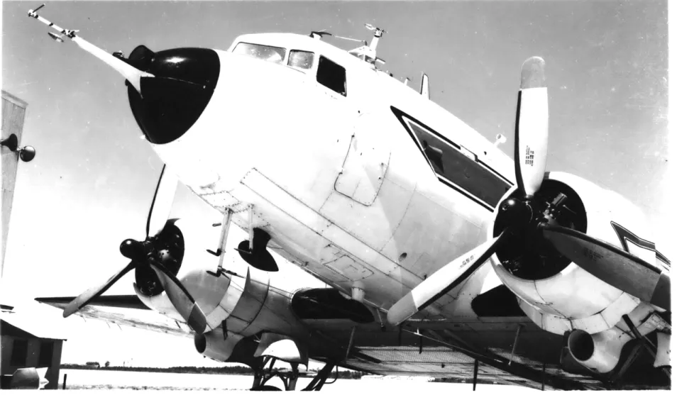
-windshield of the Woods Hole C47 (Figure 4). According to Singleton

and Smith (1960) this position was poor. They sampled clouds with

coated glass slides from two aircraft. In one aircraft the slides were exposed in a position just aft of the windshield on the cabin roof, whereas in the other they were exposed nearer the nose. Samples

taken by both aircraft, flying one behind the other, in the same cloud indicated twice as much water on the roof-mounted slide as found on the nose-mounted slide. To compare nose and cabin exposures of the hot wire instruments a duplicate pair of instruments were mounted on a boom projecting 3 feet from the nose of the C47 (Figure 4).

During a field trip towards the end of May, 1962, the two exposures were compared by operating the two sets of instruments simultaneously. Comparison of simultaneous deflections obtained by the two sets of instruments, after allowance for differences in gal-vanometer sensitivity, led to average deflection ratios (cabin to nose) of 1.64 for the cloud and 1.48 for the precipitation instrument. The difference in response can perhaps be accounted for either by trans-port of water from the aircraft surface to instrument level by eddies

separating from the windshield or by concentration of the drops due to inertia effects. Data from the cabin installation obtained before May, 1962, were corrected with the above factors.

9

-3. Procedure for wind tunnel calibration of liquid water instruments.

The two instruments were quite simple to build, but their calibration was difficult. Inasmuch as no well-established pro-cedures for liquid water content instrument calibration exist, the writer was forced to develop them. Experimentation with a small tunnel of circular cross section 3k" in diameter built by the writer at Woods Hole gave him the necessary experience, which is briefly summarized as follows:

A single spray gun produced a strong liquid water concentra-tion near the center, a characteristic of nozzles using compressed air to atomize the spray. Attempts to smooth out the water dis-tribution by a mixing chamber in front of the bell mouth resulted in unpredictable and unmeasurable losses to the tunnel walls. The expedient of metering the water flow and injecting the water spray

so that none was lost to the tunnel walls was finally adopted.

There was still the problem of having a reasonably flat spray distribution across the tunnel cross section. Ideally the distribu-tion should have a rectangular or top-hat profile, but obviously this ideal can only be roughly approximated. A fairly flat but irregular distribution was finally achieved with a circular array of

commer-cially available nozzles, which required compressed air to atomize the spray. These were mounted just in front of the tunnel bell mouth. The air pressure applied to the nozzles was used to control the drop

size.

Since the responses of both instruments were dependent on drop

-- 10

-size, a shadowgraph technique of photographing the drops in the

tunnel was developed to estimate the drop size distribution. Earlier use of the above technique by McCullough and Perkins (1951) for photo-graphing cloud drops from aircraft had been complicated by the rela-tively long light pulse duration of spark sources then available. Very high-speed spark sources have recently become commercially avail-able so that the technical problem of shadowgraphing drops moving at aircraft speeds is greatly simplified. A simple box camera was built, and a commercial high-speed spark source was modified somewhat to

shadowgraph droplets in the tunnel.

The final calibration of the instruments was done at a tunnel belonging to the Air Force Cambridge Research Laboratory at Hanscom Field. It had a square cross section of 6x6 inches. This cross

section - larger than the author's three-inch tunnel - was

con-sidered better with respect to tunnel wall interference and spray plume size. The circular array of nozzles was placed just outside the bell mouth, centered at the tunnel axis and pointing slightly inward. The

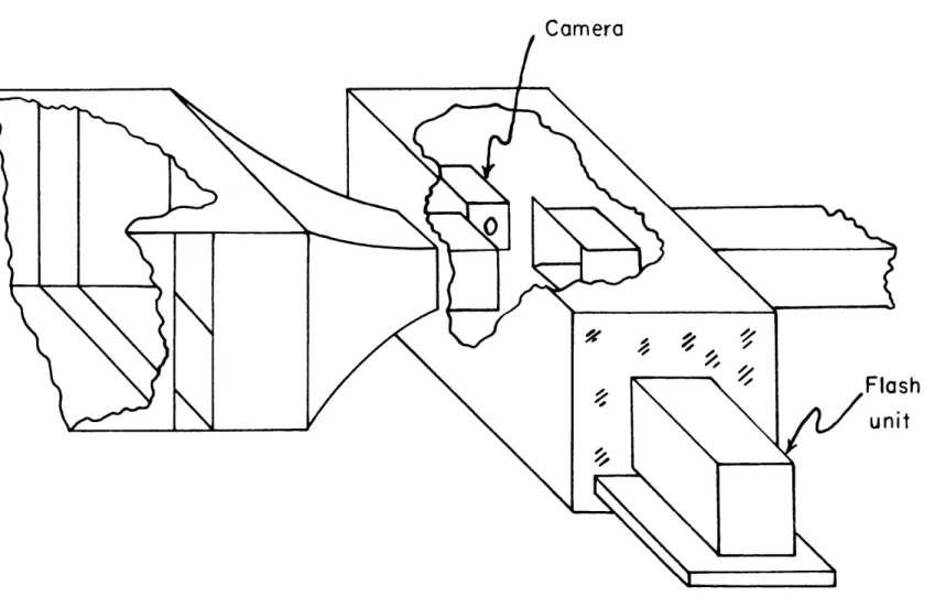
arrangement of the instruments in the tunnel is shown in Figure 5 and the shadowgraph equipment is shown in Figure 6.

The technique of calibration consisted of exposing the instru-ments to systematically varied combinations of water flow rate and air pressure. Shadowgraph pictures (Figure 7) were taken of the spray at various flow rates and air pressures, corresponding to the exposure

- 11

-instruments were not exposed simultaneously. The exposures had to be separated, because the test section was too small to accomo-date both the instruments and the shadowgraph apparatus.

The spray density varied with position in the tunnel cross section but was confined to the inner 5x5 square inch cross section. The cloud instrument readings were therefore taken at each of 25 points in a square array as illustrated in Figure 8. The average liquid water content in gm/m3 then was computed on the basis of the water flow rate, the grid cross section area (25 square inches), and the air speed.

The precipitation instrument was exposed only at the tunnel center because of its larger size. The liquid water concentration in the cross-sectional area covered by the precipitation instrument head was assumed equal to the total liquid water multiplied by the ratio of the average cloud instrument reading taken at 5 grid points grouped about the tunnel center to the average reading at all 25 points.

The storage batteries which supplied the electric current to the instruments were connected in parallel with a DC power supply.

The power supply output could be adjusted so as to maintain a particular voltage across the instruments independent of the current drain.

When the instruments were exposed to the spray, the fluctuations in spray density caused slight voltage fluctuations of less than 0.1 volt. Systematic errors due to voltage drops at high current drains were thereby eliminated.

- 12

-4. Volume median drop diameter and liquid water content as established from shadowgraph pictures.

A total of about 400 photographs were taken to obtain adequate samples of the drop population at each combination of water-flow rate and air pressure. A total of 48 different combinations of

flow rate and air pressure were used so that on the average about 8 pictures were taken for each spray condition. Three different camera lenses were used to vary the magnification (3.5, 5.1, and 10.1 times) according to dominant drop size. The problem of sizing and counting the drop images was so considerable that the author was motivated to find a convenient technique for doing the job.

This technique was centered around a commercially available image-splitting microscope eyepiece. Since only a rather low magni-fication was needed to look at the films, the image splitter was mounted on one end of an optical bench lined up with the film at the other end. A negative lens mounted between them formed a

Galilean-type telescope with the image-splitter eyepiece. The field of view and magnification were regulated by moving the negative lens and

film. The best compromise between field of view and magnification was obtained by viewing the film a quadrant at a time. A rectangular

grid was superimposed so that the eye would not get lost while counting drops.

Instead of measuring every drop to establish the drop size distribution, a less laborious,but somewhat less exact method was

I_-- 13

-adopted. The set of pictures for a given spray condition was

in-spected to determine the maximum drop size. The image-splitter micrometer was used to measure this maximum drop diameter and set at half the maximum size. The double drop images in the field of view could then be counted in two groups, greater than or equal to and less than half the maximum drop diameter, by noting whether or

not the images overlapped.

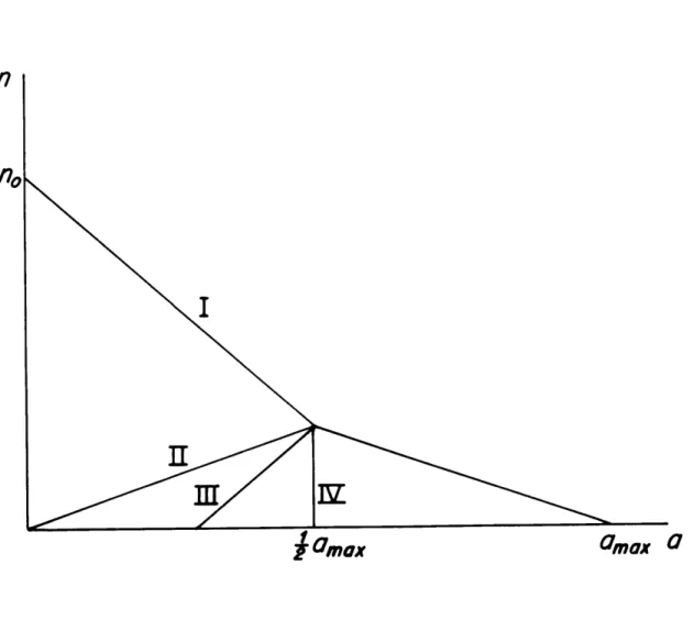
The volume median drop size was computed on the basis of a simple model of the drop size distribution (see Figure 9). Let N₂ and N1 represent the numbers of drops larger than or equal to and

less than half the maximum drop diameter, respectively. In the assumed model distribution, the frequency distribution function n is given in terms of the drop radius a. amax is the maximum drop radius, for which n is zero. The actual distribution function, which was

probably a skewed bell-shaped curve, is represented by a bent line consisting of two straight-line segments as shown in Figure 9. The equations for the straight lines are

and

YJ 1 y (2)

Multiplication of equations (1) and (2) by Yl padaIU and integration from 0 to amax leads to the equation for total liquid water content

- 14

-/

(.oI

0

/

3t.JLv

(3)

where /0 is the density of water, , that of air, V is the volume photographed, and R is the liquid water mixing ratio. The volume median radius is denoted by am and is such that half the total liquid water content is contained on either side of am. Evaluation of the integrals of 1pa3nd/ afrom 0 to am and from am to amax, which equal lead to the fol-lowing relation between N1/N₂ and am/amax

and

N1/N2 was evaluated for various assumed values of am/amax, the

results of which are graphed in Figure 10. Four different straight lines are given in Figure 9 for a amax, where cases I, II, and III represent the model distributions for N1 , = , and N₂, respectively, and case IV represents NI = 0. Equations (4) and (5)

N₁

take care of cases I and II with N- ranging from 1 to oo am

and amax ranging from .7 to .308, respectively. For N₁ = 0, am

is .725. It is not necessary to compute case III, since the amax

N1 N1

points corresponding to -- = 1 and - 0 are so close together.

N2 _N

- 15

-The droplet count data derived from the shadowgraphs may be used to evaluate liquid water content with the aid of equation (3). To do this the volume V must be found by multiplying the depth of focus by the area photographed.

To evaluate the depth of focus a drawing of several parallel lines of graded thickness were photographed and transferred, reduced in size, to a photographic plate. This plate inclined at an angle of 450 to the focal plane plate, was shadowgraphed with its center in the center of the drop camera's field of view so that the lines on the plate cut diagonally across the focal depth. The focal depth of each lens was evaluated from the measured lengths of the sharp parts of the line images. Then the volume of sharp focus was com-puted for each lens to be .77 + .08, .25 + .03, and .17 + .02 cm3 for the 127, 90 and 50 mm lenses, respectively. The cloud instru-ment, because of its one-second response time, averaged over a volume of approximately (1.9 + .4)x103cm3.

The results of computations with equation (3) are summarized in Figure 11, where the liquid water contents computed are plotted against values of the average liquid water derived from the flow meter readings. The latter were corrected for non-uniform distribu-tion of liquid water across the secdistribu-tion by using the cloud instrument responses (as illustrated in Figure 8) to estimate the liquid water present in the volume photographed. There appears to be a systematic dependence of variance on the lens used, which may be due to the combined effect of a bias toward counting the large drops in an effectively

- 16

-larger volume and the tendency to lose the small drops by smearing out of the image because of the drop motion. The liquid water contents derived from the photographs are well-correlated with the values derived from the water flow rates, but the scatter from the line of equality is about 6 and .06 times the flow rate values. The largest part of the variance is probably due to sampling errors resulting from small-scale fluctuations in space and time of the liquid water concentration.

5. Graphical analysis of data to obtain calibrations.

The maximum and volume median diameters (the latter read from Figure 10) were plotted against water flow rate for each value of air pressure. Empirical equations were fitted to the data in such a way that extreme values were generally enveloped by the resultant straight lines for each nozzle air pressure. The results are summarized in Figures 12 and 13. The empirical equations fitted the data reasonably well except for the lowest pressure of 5 lb/sq.in. The anomalous behavior of the data at 5 lb/sq.in. probably was caused by settling out of the larger drops on the bottom bell mouth wall, which was observed to be badly wetted by the spray. At higher air pressures

the wetting of the wall was negligible.

Then Figures 12 and 13 were used to obtain the maximum and

volume median drop diameters contained in Table 1. The data in Table 1 were grouped in 4 sizes and averaged as indicated by the zig-zag lines. This grouping made the wind tunnel data more manageable in the

- 17

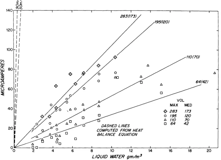
-cal construction of -calibrations. The average galvanometer current for each average liquid water content (determined from the flow rate) and drop-size group were evaluated and plotted (Figures 14 and 15)

to give calibration graphs for the cloud and precipitation

instru-ments. Inasmuch as there was no systematic non-linear behavior apparent within the accuracy of the data, straight lines through the origin were drawn for each drop-size group. These lines are of the form

= 'I (6)

where A is the current (in microamps), 4w- is the liquid water (gm per cubic meter) and

3

is a function of'drop-size, different for each of the two instruments. As shown on Figures 15 and 16 S decreases with drop size for the cloud instrument and increases .. for the precipitation instrument. From these lines the volume median drop diameter as a function of cloud to precipitation instrument current ratio was found and is given in Figure 16. With either of the calibrations and Figure 16, volume median drop diameter and cloud liquid water may be found from the two instrument readings. First the volume median drop diameter is evaluated from the ratio of the instrument responses. Then the liquid water content is found from either one of the calibrations by the line on the graph corresponding to the volume median diameter.

Empirical and theoretical instrument response efficiencies are shown in Figure 17. The former are defined by the ratio of the drop-size function *5 in equation (6) to its maximum value.

- 18

-I

Theoretical collection efficiency curves are also plotted for the

cloud instrument and a prolate ellipsoid close in size to the pre-cipitation instrument. These curves are based on the computations

by Brun and Mergler (1953) and Dorsch, Brun and Gregg (1954). The

theoretical collection efficiency of the cloud instrument is shown only for drop diameters less than 30 microns, because drops larger than 30 microns tend as their size increases to be less efficient in cooling the wire because of incomplete evaporation. For example, drops 500P or more in diameter are larger than the wire and may be

sliced through with very little cooling effect per unit mass of water. On the other hand, the theoretical collection efficiency of the

prolate ellipsoid is remarkably close to the response curve of the precipitation instrument, since the slicing effect has been eliminated

by the ceramic backing.

6. Solution of the boundary value problem of the cloud instrument

in dry air.

The solution of the steady-state boundary value problem of a wire heated by an electric current is given by Carslaw and Jaeger

(1959). The wire temperature gradient is assumed to be only along the wire because of its thinness. The differential equation of the

heated wire is

w"- iC t dO

(7)

- 19

-primes represent derivatives with respect to X , the distance along the wire. The constants are

.239q 2 rw

w'K

and

where

IL

is the current in amperes, iwo the specific resistivity of the wire in ohm cm at air temperature, W the wire cross section area in cm2, o( the temperature coefficient of resistance in OC-'

h

the turbulent heat transfer coefficient in cal cm'2sec- OC-l,

K

the conductivity of the wire in cal sec-1 OC-1cm-l, and Q-,

the wire radius in cm.

'A

is positive in the computations of interest. The solution of equation (7) which satisfies the boundary

conditions 3=O, X = 0 o' L

is

C

where L is the wire length.

The equation for the potential gradient along the wire is

a d sol tL (9)

and its solution

- 20

-Computations based on equation (8) and values of h derived from empirical data given by McAdams (1942) are summarized in Figure 18. Table 2 contains values of h as a function of y and air speed. For approximate computations both

h

and a< were assumed constant. When

y

approached a value of 6000C, the constant a< was taken as zero, and an appropriate value of the resistivity ,w

substituted for tw, in equations (7) to (10). The numerical values of the parameters contained in equations (7) to (10) are

summarized in Table 3.

Figure 19 gives a comparison of the computed curves of current as a function of voltage with measured values. This comparison makes the wire temperature profiles given in Figure 18 more credible. Note that the wire temperature gradients in Figure 18 are mostly confined to regions on the ends, 0.6 cm in length.

Therefore, in the case of the dry wire, the assumption by Neel of a uniform temperature was quite reasonable. In the case of the wet wire, however, as evident from the redness observed in a small region near the center of the wire, the assumption of uniform temperature is not justified. Nevertheless, for purposes of comparison with the

empitical tunnel calibrations, computations based on Neel's heat balance equation have been carried out for both instruments.

7. Results of heat balance computations.

The equation for liquid water content as a function of current, voltage, and wire temperature is given by Neel:

--- 21

-.23qlE

hAsY

(11)

/O

VA rH

V ,H

where

I

is the current in amperes, E the voltage,

V

the air

speed in cm/sec, Ap the projected area of the instrument on a plane normal to the air flow in cm2,

H

the enthalpy of water at air temperature in cal/gm, and A. the surface area of the wire

in cm2. Equation (11) is based on the assumption that all the water that impinges on the instrument evaporates. From wind-tunnel

measurements of

I

and

E

for zero liquid water and appropriate

values of the constants, the values of

h

were computed by the writer to be .027 and .034 cal(cm2 OC sec) - at air speeds of 50 and 90 m/sec, respectively, which agree with Table 2 well within

the 20% accuracy specified by McAdams for his empirical curve on p. 221. The constants for both instruments are given in Table 4.

The liquid water contents corresponding to various values of instrument current and the operating voltages (1.65 volts for the cloud and 28 volts for the precipitation instrument) were computed.

From the resistances

E/I

the values of

j

were established by

reference to a resistance-temperature curve. Since the dependence

of 6 on temperature is rather weak, the dry air values already

computed were used.

The results of the above computations are superimposed on the calibrations given in Figures 14 and 15. The evidence indicates very definitely that all the water impinging on the instruments is not

- 22

-levaporated, since the observed readings are less than the heat balance computations predict. This is especially true for the precipitation instrument. The computed heat balance curves are quite linear, which agrees with the behavior of the tunnel data within their accuracy; but they are strongly dependent on air speed. However, an examina-tion of the tunnel data (not shown) did not confirm such a dependence. Therefore the evaporation efficiency of the instruments must vary in such a way as to nullify the air speed dependence. Such an effect is physically quite plausible inasmuch as the water residence time on

the instruments varies inversely as the air speed.

8. A slight digression.

The development of a red hot spot in the middle of the cloud instrument wire when exposed to liquid water has already been mentioned. Similarly the precipitation instrument has also been observed to develop irregularly placed red hot spots mostly towards the rear of the cone when exposed to very large liquid water contents (the extremes used

in the calibration). The hot spots have already been related to the tendency for water drops to ride on a cushion of steam over a hot enough surface. An experiment has been performed with a heated plate which indicates that the transition temperature from boiling with intimate contact to compact spherical shape without contact of a water drop on a hot plate is about 250 to 3000C.

The way in which the wire can be heated to red heat (about 9000C) at its center and still average cooler than the dry wire is

--9-LlllllsYI^--

- 23

-illustrated in Figure 20. The wire near the center, which is above 2750C, is not cooled by evaporation. As the liquid water

is increased from zero the wire center begins to gradually glow

dull red. Then as the water flow increases the center glows brighter and is more concentrated. At the extreme water flow used, the wire

sometimes was cooled so much that the red spot was quenched. The quenching of the red spot was first noticed when some calibration readings ran off scale. Sometimes during a measurement the reading appeared on scale at first but then fluctuations forced

the galvanometer off scale. Apparently at extreme liquid water contents the wire was in a metastable state which could be triggered by the liquid water density fluctuations normally occurring in the

tunnel. After quenching the wire could be returned to the high temperature regime only by drastically reducing the liquid water.

The wire at high liquid water contents was found inadvertently to constitute a simple physical system which is a climatological analogue. The two states of the wire may be looked upon as analogous to an ice age and a warm age. The finite amplitude fluctuations of liquid water content which trigger the system from one state to the other are analogous to hypothetical fluctuations which possibly trigger the earth's atmosphere from one climatological state to the other.

- 24

-9. Accuracy and response times of the instruments.

In the calibration curves of Figures 14 and 15, the errors are practically confined to fluctuations of liquid water content in space and time. The error due to fluctuation of tunnel air

speed is at most + luamp. Therefore all calibration curves must

go through the origin. Some of the error may be the result of neglect-ing the possible non-linearity and dependence on air speed of the

instruments' performance, but as already mentioned these factors were not apparent in the data. Therefore the error analysis was based on the standard deviations of the individual points from the lines as drawn. The average standard deviations are 18% and 30% for the cloud and precipitation instruments, respectively. The corresponding probable errors are 12% and 20%.

On the basis of the above probable errors, the probable error of the ratio of cloud to precipitation instrument response and hence the probable error of volume median diameter can be determined. The probable error of the ratio is approximately the sum of the errors of

the two instruments, which is 32%. By taking extremes of the ratio

based on its estimated error, an estimate of the probable error of volume median drop diameter was established to be 29%.

The response times of the two instruments have been made amply evident both from wind tunnel work and aircraft use. The cloud

instru-ment response time was found to be 1 sec (the time required to reach

63% of its full-scale value in response to a sharp change in liquid ~_II~ I

- 25

-water) and is entirely a function of wire diameter. The response time of the precipitation instrument is more complicated in nature, since its response is conditioned by the ceramic cone as well as the wire size, and was evaluated to be 3 sec. This response time may appear short for a large mass such as the ceramic cone, which

is quite apparent in the warm-up time of the instrument (considerably larger than 3 sec); but actually the wire and the ceramic surface immediately under it are most influential in establishing the response time to changes in liquid water content.

- 26

-References

Brun, R.J. and H.W.Mergler, 1953: Impingement of water droplets on

a cylinder in an incompressible flow field and evaluation of rotating multicylinder method for measurement of droplet-size distribution, volume-median droplet droplet-size, and liquid-water content in clouds. NACA TN 2904, 71 pp.

Carslaw, H.S. and J.C.Jaeger, 1959: Conduction of heat in solids.

Oxford University Press, London, 509 pp.

Dorsch, R.G., R.J.Brun, and J.L.Gregg, 1954: Impingement of water

droplets on an ellipsoid with fineness ratio 5 in axisymmetric flow. NACA TN 3099, 50 pp.

McAdams, W.H., 1942: Heat Transmission. McGraw-Hill, New York, 459 pp.

McCullough, S. and P.J.Perkins, 1951: Flight camera for photographing cloud droplets in natural suspension in the atmosphere.

NACA RM E50KO/a.

Neel, C.B., 1955: A heated-wire liquid-water-content instrument and results of initial flight tests in icing conditions.

NACA RM A54123, 33 pp.

Neel, C.B. and C.P.Steinmetz, 1952: The calculated and measured

per-formance characteristics of a heated-wire liquid-water-content meter for measuring icing severity. NACA TN 2615, 59 pp.

Singleton, F. and D.J.Smith, 1960: Some observations of drop-size

distributions in low layer clouds. Quart.J.Roy.Meteor.Soc.

86, 454-467.

Wilson, E.B.Jr., 1952: An introduction to scientific research. McGraw-Hill, New York, 375 pp.

- 27

-Table 1

Maximum and volume median drop sizes for various spray conditions. (Broken lines represent grouping boundaries).

Pressure b/sq.in. Flow cc/min. 117 174 230 287 414 545 5 10 15 20 30 Max 230 Med 120 Max 245 Med 138 Max 260 Med 151 Max 277 Med 164 Max 310 Med 192 Max 348 Med 220 Group 1 204 100 220 122 230 136 245 150 310 218 (Max 283 Avg IMed 173 160 135 104 80 68 54 174 145 110 97 82 66 185 155 120 108 92 74 195 165 130 120 102 82 220 185 145 147 126 102 250 210 165 174 150 120 Group 2 (Max 195 120 40 60 80 85 65 50 44 34 28 95 70 55 56 43 36 100 75 60 62 48 40 105 80 65 70 54 46 123 95 75 86 68 58 140 108 88 102 82 70. Group 3 Max 110 Avg Med 70 Group 4 Max 64 Avge Med 42

- 28

-Table 2

h in cal/cm2 oC sec as a function of airspeed and wire temperature.

y/air speed 00C 200 400 600 800 1000 48 m/sec .025 .027 .029 .031 .033 .034 90 m/sec .035 .037 .041 .043 .046 .049 Table 3

Values of constants used in equations (7) to (10).

h = .027 (air speed 48 m/sec) h = .037 (air speed 90)

cal/cm2 oC sec K = .067 cal/sec cm OC 0( = 7.0 x 10-3 r .. = 2.06 x 10- 5 ohm cm L = 4.1 cm a.= .0255 cm W = 2.06 x 10 - 3 cm2 r. = 5.3 x 10-5 ohm cm(S(-O) Table 4

Constants used in equation (11) H = 580 cal/gm

Cloud instrument

As = .659 cm 2

Ap = .209 cm2

h = .027 (air speed 50 m/sec)

V = 5.0 x 103 and 9.0 x 103 cm/sec Precipitation instrument 34.4 cm2 20.2 cm2 .011 cal/cm2 oC sec oI It II " 7 " ) .016 - Ill.

"

_{= .034 ( "11}

i

g

Figure 1. From left to right are shown the 28 volt precipitation instrument

Ammeter

o0-

25

omps.

Voltmeter

o-

30

volts

28

volts

Ammeter

0-

25

amps

Figure 3. Precipitation instrument bridge circuit.

Figure 4. Duplicate nose and cabin installations of liquid water content instruments on Woods Hole C47 aircraft.

MOUNT MOVABLE

IN TWO DIMENSIONS ACROSS

TUNNEL

HOT WIRE

Camera

Figure 6. Shadowgraph equipment mounted to photograph spray drops in tunnel.

Flash

Figure 7. A shadowgraph of spray drops at center of tunnel cross section. (Original magnification 3.5X, enlarged approximately 2X).

Air speed 123 knots

Water flow 108 cc/min

Avg.

liquid water content 1.76 gm/m

3

Air pressure 12 psi

Avg. deflection 5.2mamps.

Max. drop diameter 240,

2

3

4

K

il17. 7 1 17 I 7 7 I

Air pressure 80 psi

Avg.

_{deflection 9.8 amps.}

Max. drop diameter

35,q

0 1 2 5 2 I 6 10 10 2 6 12 12 14 5 13 16 15 16 7 I 2 2 5 3 I 2 3 4 5

Tunnel

wall

Water

flow 414 cc/min

Avg. liquid

water

content 6.75

gm/m

3

Air pressure 12 psi

Avg. deflection 14.6 pomps.

Max.drop

diameter 450A

0 0 0 0 I 2 4 2 3 -1 10 32 24 21 8 10 30 30 36 8 -3 -I - 7 4 2 3 4

Air pressure 80

psi

Avg. deflection 22.9

omps.

Max.drop diameter 160,u

0 4 4 9 2 4 21 30 24 I 13 38 44 44 10 26 44 43 43 18 4 10 6 10 6 I 2 3 4 5

Figure 8. Examples of cloud instrument data obtained at the Hanscom Field spray tunnel. The numbers are bridge current readings in microamps at grid points in the tunnel test section for four different

combinations of water flow and air pressure. 5 4 3 2 I O i I I i 2 4 6 6 2 7 18 15 15 6 0 6 5 6 4 -I -I -I -I -I I

I

II

II

j

Gmox

am

x 0

Figure 9. Model drop size distributions. Cases I, II, and III represent

N1> , =, and

<N

2, respectively. Case IV is N1 = 0.

no

IV

---

~---

~

10

20

30

40

50

60

70

80

90

Af/N

Figure 10. am/aa _x as a function of N₁/N₂.

33L

39 -Io 10 /

1

S0.5-1 C 0- 0 1 O X1o 05, _o _ 127 mm LENS S0 90 mm LENS -A 50 mm LENS 01 005 .001 1 ₁₀ 20 ₃₀

WEIGHTED

AVERAGE LIQUID WATER CONTEN

T

FROM

INPUT

FLOW

Figure 11. _{Comparison of weighted average liquid water content with values} computed from shadowgraph drop counts.

500

0 5psi

_5psi

S

~o10

015

400

- A 20

030

A 40

-t--- 5psi

k 60

_10psi

K300

-

80

...

_{15 psi}

k 200 - ps

-40psi

100- 60psi

10080psi

gb 8

12 12.5 16

20 sbl2 12.5

16

20

0 1 . 1 1 1 I l _i

0

100

200

300

400

500

600

WATER FLOW cc/min.

Fig. 12. Maximum drop diameter of tunnel spray from shadowgraph pictures as a function of water flow input and nozzle air pressure. Data fitted subjectively with equation

S .79W + 655 _{- 33}

2ama_{x -33}

where W is water flow rate in cc/min and P is air pressure in lb/sq.in., except for pressure of 51b/sq.in.

0 2 4 6 8 10 2 14 16 18 20

LIQUID WATER gm/m3

Figure 14. Calibration of cloud instrument over air

176 knots.

LIQUID WATER g/m 3

Figure 15. Calibration of precipitation instrument over air speed range from 95 to 176 knots.

-N

2.0

8

₀

•

1N0 - _ - ----

--10 50 100 500 1000

VOLUME MEDIAN DROP D/AME TER IN M/CROWS

Figure 16. Ratio of cloud to precipitation instrument bridge current as function of volume median drop diameter.

of

4O

0-

_ _ __ _ _ _ _ _ _

=z1

0

0

00

10

VOUEMDA

RPDIMTRI

IRN

Fiur 1. ato fcludtoprciitt oisrmtbidecrnta

0.8

CLOUD INSTRUMENT

02/

0

1 _5 10 50 100 500 1000

VOLUME ME4

/AN

ROP DINSAMETER

Figure 17. Instrument response efficiency as a function of volume median drop diameter.

" //

1

2

X cm

Figure 18. Theoretical temperature profiles of cloud instrument hot wire in dry air.

400

300

0

200

100

0

800

600

o400

200

OL

0

18 FOR Ga=O 16- o 10 AND r =53 A/R SPEED o 90 M/SEC o 14 -14 4 0o AIR SPEED 48 M/SEC 12 8

6

I I I I I 0 1.0 2.0 3.0

VOL TAGE

Figure 19. Comparison of computed and observed current-voltage relationship for dry cloud instrument.

X /N cm

Figure 20. Hypothetical temperature profile of wet cloud instrument hot wire as compared with corresponding dry wire.

- 49

-PART II

Dynamics of Cumulus Convection

1. Historical introduction.

Theoretical analysis of cumulus convection essentially

started with the "parcel" concept, which is still very much with us in meteorological thermodynamic charts and in many textbooks on

meteorology. More recent developments in cumulus convection have their origin in the work of Stommel (1947, 1951) and Houghton and Cramer (1951) on entrainment in cumulus clouds. The impetus for Stommel's

work came from aircraft observations of trade-wind cumulus by McCasland

and Woodcock during the 1946 Wyman Expedition to the Caribbean

-summarized in a monograph by Bunker, Haurwitz, Malkus and Stommel (1949). In Stommel's work and some of the later work, the cumulus cloud was modeled as a steady-state jet. In contrast, Scorer and Ludlam

(1953), while accepting the entrainment notion, proposed a "bubble" model for convective elements. This was based on impressions gained

from conversations with glider pilots. Scorer (1957) combined tank experiments and dimensional analysis to arrive at a rational development of the "bubble" or "thermal" model in a neutral environment. Both the steady-state jet and "bubble" models are essentially modified parcel theories, which allow for mixing of the parcel with environmental fluid.

Concurrently with and following Scorer's tank experiments, others performed more detailed experiments. In particular Woodward (1959) and Saunders (1962) used neutrally buoyant particles to demonstrate the

- 50

-like Hill's spherical vortex. Turner (1957, 1963) explored the behavior of buoyant vortex rings and in later experiments introduced the equivalent of latent heat release.

An additional variation on the experiment theme was introduced by Malkus and Witt (1959) in their numerical convection experiments, which was followed by similar and more carefully-done experiments by Ogura (1962, 1963) and Lilly (1962, 1964). All the numerical experi-ments had certain features in commnon, namely, (1) use of the equations of motion, continuity, and thermodynamics, (2) an assumed eddy coeffi-cient of viscosity, and (3) assumptions concerning the initial con-ditions. In general the numerical experiments do not support the

existence of bubble-like elements in a conditionally unstable atmosphere, but neither do they support the steady-state jet model. Ogura's

experiment in particular appears to lean more towards an expanding jet with a mushroom-like structure.

An alternate form of numerical analysis has been based on the assumption of some sort of steady-state jet or "bubble" model

circula-tion. For the steady-state jet model, computations have been made on the basis of continuity, thermodynamic, and buoyancy conditions averaged over the jet cross section. The prototype computation has been that of Houghton and Cramer followed by Haltiner (1959), and Squires and Turner (1962). In the case of the bubble model, a simple form such as a sphere has been assumed for an isolated element rising under the

influence of buoyancy resulting from the effect of condensation and some assumed law of entrainment. Examples of such computations are

- 51

-those by Ludlam (1958), Levine (1959), and Mason and Emig (1961). The above numerical analyses may be designated as parametric entrain-ment models.

In general all the theoretical work is based on the same basic equations of motion, continuity, and thermodynamics; but the complex

interactions involved make the isolation of unique boundary value problems impossible. Therefore each school of thought has tended to develop approximate techniques and notations with only a superficial regard for each others' work. An attempt will be made in the following sections to bring some sort of unity into this work.

Possibly the tank experiments with the various forms of buoyant blobs and jets have been most helpful in giving physical insight into the forms of turbulent motion assumed by transient buoyant fluid impulses in a neutral or stable environment, but the problem of extrapolating laboratory experiments to extremely irregular cumulus convection is not at all a simple one.

The numerical experiments by Ogura (1962, 1963) appear to have been most effective so far in yielding some insight into the form that atmospheric convection elements tend to assume in neutral, stable, and unstable environments. Yet even in Ogura's numerical experiments the conclusiveness of the results is limited by the assumption of a constant eddy viscosity coefficient and the limited grid network dictated by the limitations of machine capacity. A feature of Ogura's work (1962), which makes his later results credible is his success in partially

reproducing the detailed behavior of buoyant elements in tank experiments.. . -- 11I^--II II1_I ~LI _~I -- I I--- _ ._1 -.--II ~^-~)---- ---~I_ __ II I_^__

- 52

-#2. Comparative analysis of tank experiments in terms of the author's bubble model.

Instead of treating the various parametric entrainment models in chronological order of introduction, the simplest mathematical treatment is taken first. The analysis and notation advanced by

Scorer (1957) has been adopted by others largely due to its simplicity and empirical success. By dimensional analysis Scorer deduced the equation

W2 C2gBr (1)

for the vertical velocity W of. a thermal where C2 is essentially a Froude number, g the acceleration of gravity, and r the radius of

largest horizontal cross section. B is the average buoyancy defined as the ratio of average density excess to the environment density.

In tank experiments the outline of the model thermal was usually followed by the dye contained in it. Therefore, although the buoyancy decreased with time, the product of buoyancy and volume BV was con-served so that BV = BoVo, where Bo and V0 are the initial buoyancy

and volume, respectively.

By setting W dZ where W is now considered to be the vertical dt

velocity of the center of mass of the thermal and Z its vertical coordinate, Scorer derived the equation

t = kZ2 (2)

by integration of equation (1). The constant k is given by __ _~_I~ _~ _ ___~ _~__I I~_

- 53

-k = m /2nC(gBoVo) (3)

where m and n are constants by virtue of the assumption of similarity. The constants m and n are constants of proportionality with the

equations n -r and m - V r

Obviously if m, n, and C are constants, then k(BoVo) is a constant

and the constant

mk

2nk(BoVo)

Thus the combination of Scorer's dimensional analysis and assumption of similarity defines the thermal's behavior entirely in terms of a

simple constant parameter n.

Scorer's analysis may be very simply shown to be the equivalent of the writer's 1959 analysis in which he assumed rates of mass entrainment

and detrainment, K. -_Pe and Kd

W

_r , respectively. From the conservation of mass constraint on a spherical thermal and these assumed mixing laws the writer derived the equation

dr

_{- =}

k e-kd

_e

_W.

₍₅₎

Iot 3

Integration of this equation yields the linear equation

r

e

-

(6)

- 54

-where ke and kd are coefficients of entrainment and detrainment, res-pectively. For the tank experiments in a neutral non-turbulent environ-ment, the detrainment parameter is probably zero, and we can then relate

ke to Scorer's n

ke 1

-9

3 n

considering r >> ro

(For a turbulent or stable environment the introduction of kd may be appropriate, however.) Then an equation for the conservation of momentum was written essentially as

01 ,+o<

M3 M

B

-

./%I

W

r (7)

dt"

where M is the mass of the thermal element and

Q(

is the apparent mass coefficient due to acceleration of the surrounding fluid. (Relative acceleration of the internal fluid is neglected.) The viscous drag on

the thermal has been assumed entirely due to turbulent mass exchange between the thermal and static environment. Then since

M =(-(8)

Ct

equation (7) reduces to

1W

=

-

,

?

o

W

(9)

In the case of the tank thermals the equation for conservation of buoyancy may be written as

-MB

-1

(10)

dt

IC1

- 55

-which by equation (8) reduces to

--

_=-

WE

Then.since _

equations (9)

and (11) may be written as

equations (9) and (11) may be written as

LW

--x a

(11)

(12)

-B

r

r

1+-<

r

and

c

/_

e"

In the case of a neutral environment (kd = 0) the solution of equation (13) is by substitution from equation (6)

(13)

(14)

where

₃

h F

5 1+3 t.

Substitution of equations (14) and (6) in equation (12) makes possible its integration so that

(,[1- Call

Now to compare equation (15) with Scorer's equation (1), we set Wo = 0 and neglect the f-term, which is justified if -~ ± 1.

3

ve;

.Substitution from equation (14) for Bo in equation (15) results finally in

W

=

33

r

(16)

2(

+,)

ke

(15)

1~-_~_111~ 11..

.I--^..I .^..

3 13o

WZ _{w'= 2}

- 56

-This is of the same form as Scorer's equation (1).

For a sphere, c< is (Menzel, 1960, pp.2 2 8 and 229), so

that the coefficient C2 of Scorer's equation (1) by comparison with

equation (16) is A~e = /3 . According to Scorer's (1957) experi-ments, 11 is-approximately 4, which gives us the values fg = .75 and C = .11.33 = 1.15. This agrees well with Scorer's experimental evalua-tion, C n'1.2. Therefore the tank experiments are consistent with the assumption of oc = and of a spherical shape. (A similar but not as detailed analysis was performed by Saunders (1962) in con-nection with his analysis of experiments on the penetration of a stable interface.)

Equations (6) and (15) may also be applied to the non-buoyant puff in the experiments described by Grigg and Stewart (1963) and Richards (1965). The buoyancy equation (14), of course, is dropped and equation (15) reduces to

W = Wo (15')

3. Internal circulation of a thermal.

The writer has derived considerable physical insight into the nature of the circulation developed in tank thermals from looking at many of the unpublished experiment photographs taken by Dr. P. Saunders and from some simple experiments of his own with potassium permanganate solutions in a neutral environment. All of the above experiments had gross features in connon. The initial density distribution was rapidly

- 57

-reformed into a bowl-like structure. In Dr. Saunders' streak photographs, the associated circulation appeared to be organized into a spherical vortex-like circulation with the dense bowl-shaped fluid concentrated at the leading surface of the thermal, as drawn by Scorer (1957). The streak photographs also indicated that the level of internal small-scale turbulent motion was at least an order of magnitude smaller than the vortex motion and the vertical trans-lation of the thermal. In the later stage of development a ring of relatively dense material appeared to be concentrated at the ring vortex axis. Furthermore the vortex circulation appeared to be very rapidly organized just after release of the buoyant material and remained constant or increased slowly thereafter.

In the numerical experiments performed by Malkus and Witt (1959), Ogura (1961, 1962), and Lilly (1961, 1962), an eddy viscosity was introduced arbitrarily which was assumed constant except by the last author. Obviously the introduction of mixing parameters in the "bubble" models discussed in Section 2 must imply some sort of eddy viscosity. An approximate analysis can be performed to establish a relation of the mixing parameters ke and kd to an eddy viscosity. This may make possible a less arbitrary choice of eddy viscosity in future numerical experiments.

In tank experiments with a neutral environment the isolated thermal or puff is essentially a turbulent mass of fluid moving and spreading into a non-turbulent environment. Turner (1963) has provided us with a study of buoyant thermals moving into neutral turbulent

- 58

--surroundings. This corresponds to the case of kd > 0. In both cases there is an average internal gradient of velocity and buoyancy, but in a still neutral environment there is no average gradient out-side the thermal or puff. In a turbulent environment an average externhl gradient of velocity and buoyancy is induced.

The average eddy fluxes of momentum and buoyancy out of a thermal or puff are related approximately to the average internal shear and buoyancy gradients by

% = -_ e- (17)

and

Fe e r (18)

respectively, where ,Ake is the internal eddy viscosity coefficient and ke the internal eddy diffusion coefficient. Since in a coordinate

system moving with the thermal the average air velocity of the sur-rounding air past it is -W, the eddy flux of momentum into the thermal

of mass

I

p

may be written as

MW

W

'be

rwA

e - the r o (19)

where ke represents the rate of entrainment. Similarly we obtain

Al

B w

*f

W.

(20)

estp

w

9 iv

- 59

-By elimination of Le and /- from equations (17) and (19)

and equations (18) and (20)

,e

=

e-

e

rW

(21)

which is the internal eddy transfer coefficient. Similarly the external eddy fluxes are

cL-A r (17')

-

"d

V

(18')

Ld"-

dPW

(19').

and

Fd P ;3 W(20')

where f represents some fraction less than one. fW and fB represent .the average external velocity and buoyancy established by the external

turbulence. The external eddy transfer coefficient is then

K

. (21')

The eddy transfer coefficients are also related to the Reynolds number of the flow defined as

S-/opw (22)

where /( is the molecular coefficient of viscosity. By elimination of W from equations (21) and (21') with equation (22) we obtain

'"e

=

/ Ae#Re

and