HAL Id: hal-03120300
https://hal.archives-ouvertes.fr/hal-03120300
Submitted on 26 Jan 2021
HAL is a multi-disciplinary open access
archive for the deposit and dissemination of
sci-entific research documents, whether they are
pub-lished or not. The documents may come from
teaching and research institutions in France or
abroad, or from public or private research centers.
L’archive ouverte pluridisciplinaire HAL, est
destinée au dépôt et à la diffusion de documents
scientifiques de niveau recherche, publiés ou non,
émanant des établissements d’enseignement et de
recherche français ou étrangers, des laboratoires
publics ou privés.
Distributed under a Creative Commons Attribution - NonCommercial - NoDerivatives| 4.0
International License
Martin Cooper, Stanislav Zivny
To cite this version:
Martin Cooper, Stanislav Zivny. Hybrid Tractable Classes of Constraint Problems. Krokhin,
An-drei; Zivny, Stanislav. The Constraint Satisfaction Problem: Complexity and Approximability, 7
(Chapter 4), Schloss Dagstuhl Leibniz-Zentrum fur Informatik, pp.113–135, 2017, 978-3-95977-003-3.
�10.4230/DFU.Vol7.15301.113�. �hal-03120300�
Martin C. Cooper
1and Stanislav Živný
21 IRIT, University of Toulouse III, Toulouse, France
2 Dept. of Computer Science, University of Oxford, Oxford, UK
Abstract
We present a survey of complexity results for hybrid constraint satisfaction problems (CSPs) and valued constraint satisfaction problems (VCSPs). These are classes of (V)CSPs defined by restrictions that are not exclusively language-based or structure-based.
1998 ACM Subject Classification F.4.1 Mathematical Logic, G.2.1 Combinatorics, G.2.2 Graph Theory, F.1.3 Complexity Measures and Classes, G.1.6 Optimization
Keywords and phrases Constraint satisfaction problems, Optimisation, Tractability
Digital Object Identifier 10.4230/DFU.Vol7.15301.113
1
Introduction
A fundamental challenge in computer science is to map out the frontier of the complexity class P, the class of decision problems that can be solved in polynomial time. The constraint satisfaction problem (CSP) is a generic combinatorial problem which includes in a natural way many important NP-complete problems such as SAT or graph-colouring. The valued constraint satisfaction problem (VCSP) can be seen as an even richer language than the CSP since it provides a general framework in which to express both constraint satisfaction problems and constrained optimisation problems. The identification of tractable classes of generic problems, such as the (V)CSP, has led not only to a deeper understanding of tractability, but also to wider application areas of well-known algorithms. Indeed, recent research has shown that very few algorithmic techniques suffice to solve all tractable language-based classes of (V)CSPs [1, 35, 40].
Many real-world problems can be modelled as classical and well-studied NP-complete problems, such as SAT, CSP or VCSP. This has the advantage that generic solvers exist which are efficient on many instances, but has the disadvantage of not taking into account specificities of the particular problem which could perhaps guarantee the existence of a polynomial-time algorithm. Obvious specificities include the type of constraints or cost functions that can occur or the structure of the hypergraph of constraint scopes. Much research effort has been devoted to identifying tractable language-based classes [2, 5] or tractable structural classes [32], with many notable successes. However, it is natural to ask whether interesting classes of instances can be defined in other ways.
∗ The authors were supported by EPSRC grant EP/L021226/1. Stanislav Živný was supported by a
Royal Society University Research Fellowship. This work was partly done while the second author was visiting the Simons Institute for the Theory of Computing at UC Berkeley. This project has received funding from the European Research Council (ERC) under the European Union’s Horizon 2020 research and innovation programme (grant agreement No 714532). The paper reflects only the authors’ views and not the views of the ERC or the European Commission. The European Union is not liable for any use that may be made of the information contained therein.
© Martin C. Cooper and Stanislav Živný; licensed under Creative Commons License BY
One way of defining classes of instances is by simultaneously placing restrictions both on the language of possible constraints (or cost functions) and on the structure of the hypergraph of constraint (cost function) scopes. Such classes are known as hybrid classes, and by extension all classes which are not exclusively language-based nor structure-based are also known as hybrid [24]. This larger meaning is the one we apply in this chapter.
As an example of a hybrid tractable class, consider a company which wishes to give bonuses to its employees (chosen from a finite set of possible amounts). Each employee has a grade, with higher grades corresponding to more important posts. Some, but not all, employees have an immediate boss to whom they report. In this case, the employee and the immediate boss must receive bonuses such that the sum of the bonuses of the employee and the boss is bounded above and below by a specified amount. On the other hand, if an employee has no immediate boss, then the rule is that they must not receive a bigger bonus than anyone at a higher grade. We will see, in Example 1, that this bonus-assignment problem falls in a hybrid tractable class.
As another example, consider the same company which now wants to assign staff to a project, minimising total salary costs while respecting constraints concerning the minimum number of personnel from each section, the maximum total number of staff on the project, as well as the availability of each member of staff. Again, we will see, in Example 4, that this problem falls into a hybrid tractable class
An important way to classify work on hybrid tractability is how classes of instances are defined. We consider the following ways of defining a class of instances of (V)CSPs:
independent restrictions on both the language of constraints (or cost functions) and on the structure of the instance.
excluding generic sub-instances (known as forbidden patterns).
properties that are required to hold after a preprocessing operation, such as establishing a certain level of consistency, has been performed.
graph properties of the (weighted) microstructure of the instance.
instances which are so strongly constrained that this implies a polynomial bound on search-tree size (or, on the contrary, so weakly constrained that there is always a solution). Historically, different hybrid classes have been identified by attempting to generalise language or structural restrictions, or to determine a large class of instances solved by a particular algorithmic technique, or to translate known results from another field, usually graph theory, to (V)CSPs. The field of hybrid tractability has not yet reached maturity and is notably lacking a general theory which would allow us to express all the above types of restrictions, together with language and structural restrictions, in a common language. Such a unified language would no doubt lead to a greater understanding and new applications.
2
Independent Language and Structure Restrictions
A constraint satisfaction problem (CSP) instance I is given by a triple éX, D, Cê, where
X = {X1, . . . , Xn} is a finite set of variables, D is a finite set of values, and C is a finite
set of constraints. Each constraint c ∈ C is a pair év, Rê, where v, the constraint scope, is a list of k variables from X and R ⊆ Dk, the constraint relation, is a k-ary relation on D.
We call k the arity of the constraint. We note that different constraints within the same instance can have different arity. The question is whether there is an assignment of values to the variables that satisfies all the constraints. More formally, to decide whether there is an assignment s : X → D such that for every c ∈ C with c = (v, R) and v = (Xi1, . . . , Xik), we have és(Xi1), . . . , s(Xik)ê ∈ R.
In language-based classes of CSPs, one restricts the set of constraint relations R on D that can appear in any instance. A finite set of relations on a fixed finite set D is called a constraint language and we denote by CSP(Γ) the class of CSP instances in which all constraint relations belong to Γ.
In structure-based classes of CSPs, one restricts the type of interactions of the constraint scopes s (by restricting the hypergraph of the constraint scopes s on X) that can appear in any instance.
We remark that an equivalent definition of CSPs is the following: given two relational structures A and B, is there a homomorphism from A to B? Language-based CSPs correspond to fixing B to a single relational structure (corresponding to a constraint language) whereas structure-based CSPs correspond to requiring A ∈ A for some (infinite) class A of relational structures [34].
In this section we will discuss known results on the complexity of CSPs that impose independent restrictions on the structure of the instance and on the constraint language.
2.1
Planarity
A constraint language is called Boolean if the domain D is equal to {0, 1}.
The incidence graph of a CSP instance I = éX, D, Cê has X ∪ C as its vertex set and (Xi, c) is an edge, for Xi ∈ X and c ∈ C, if Xi∈ v where c = (v, R).
For a Boolean constraint language Γ, we denote by CSPp(Γ) the set of CSP instances
from CSP(Γ) with planar incidence graphs and with the condition that, for each constraint in the instance, the variables in the scope of the constraint appear in the clockwise order (in some fixed planar embedding).
The complexity of Boolean planar language-restricted CSPs has recently been established. First, it was shown that, apart from Boolean constraint languages Γ where CSP(Γ) is tractable (and thus also CSPp(Γ) is tractable), CSPp(Γ) is intractable unless Γ is an even
∆-matroid [26]. Secondly, the tractability of CSPp(Γ) for even ∆-matroids was shown [38].
In order to define even ∆-matroids we need some further notation.
We use ⊕ for the exclusive or. For a tuple t over {0, 1}, we denote by t the tuple obtained from t by flipping all values; i.e., t = t ⊕ (1, . . . , 1). We say that a relation R is self-complementary if for every t ∈ R we have t ∈ R. For a self-complementary R, we denote by dR the relation {(t1⊕ t2, t2⊕ t3, . . . , tk⊕ t1) | (t1, . . . , tk) ∈ R}. We say that Γ is
self-complementary if every R ∈ Γ is self-complementary. We define dΓ = {dR | R ∈ Γ}. A set M ⊆ {0, 1}k is a ∆-matroid if for all ét1, . . . , t
kê, ét′1, . . . , t′kê ∈ M and every 1 ≤ i ≤ k
with ti Ó= t′i there is 1 ≤ j ≤ k with tjÓ= t′j such that t with ti and tj flipped also belongs to
M . (We also allow the case of i = j, in which case the new tuple that is required to belong
to M is obtained from t by flipping the ith position.) A ∆-matroid M is called even if all tuples in M have the same parity of the number of 1s. (Note that in this case i and j cannot be the same in the definition of ∆-matroids as this would change the parity of 1s.) Finally, a Boolean constraint language is called an even ∆-matroid if Γ is self-complementary and each relation in dΓ is an even ∆-matroid.
We now give an example of a constraint language that can be used to model the perfect matching problem in graphs as a planar CSP [26]. Let Mk⊆ {0, 1}kbe the relation containing
the k-tuples in which precisely one coordinate is set to one (and all others are set to zero). It is easy to check that Mk is an even ∆-matroid for every k. Let Γpm be the constraint
language on {0, 1} with dΓ = ∪k≥1Mk. It can be checked that Γ is self-complementary
and by definition dΓ is an even ∆-matroid. Hence Γpmis an even ∆-matroid. For a graph G = (V, E), we construct an instance IG = éE, {0, 1}, Cê of Boolean CSP(Γpm) with a
constraint éée1, . . . , ekê, Mkê ∈ C for every degree-k vertex of G incident to edges e1, . . . , ek.
It is clear that perfect matchings in G are in 1-to-1 correspondence with satisfying assignments to IG.
2.2
Bounded Occurrence
Another natural restriction is that of bounded occurrence of variables in the constraints. We denote by CSPk(Γ) the class of instances of CSP(Γ) in which every variable appears
in at most k constraints. Feder showed that for Boolean constraint languages that contain constants, CSP3(Γ) is as hard as CSP(Γ) [27]. Here a constant is a unary singleton relation.
On the Boolean domain D = {0, 1}, there are only two constants c0= {(0)} and c1= {(1)}.
Boolean CSPs in which every variable appears exactly in two constraints are called edge CSPs in [38] but have been long known as Holant problems in the counting community. We denote by CSPe(Γ) the set of CSP instances from CSP(Γ) in which every variable appears in
exactly two constraints. (The case of a variable appearing in at most two constraints, CSP2(Γ),
can be reduced to this case [27]). Feder showed that if Γ is a Boolean constraint language including constants such that CSP(Γ) is intractable then CSPe(Γ) is intractable unless Γ is a
∆-matroid. Tractability has been shown for several special classes of ∆-matroids [27, 21] and most recently for even ∆-matroids [38] (where the reader can find more references). For instance, CSPe(Γpm) captures precisely the perfect matching problem in graphs.
2.3
Lifted Languages
Two recent papers [39, 52] study certain hybrid classes of CSPs in which the algebraic machinery developed for the computational complexity of constraint languages is (partially) applicable. In particular, it has been shown that the complexity of the class of CSP(Γ) instances in which the structure (hypergraph of constraint scopes) is closed under inverse homomorphisms can be shifted to the analysis of the complexity of a CSP(Γ′) instance,
where Γ′ is a new, “lifted” language [39, 52]. A class of structures H is closed under inverse
homomorphisms if whenever there is a homomorphism from R′ to R ∈ H then R′ ∈ H.
Examples of such structures include classes of acyclic or k-colourable graphs. Non-examples include classes of planar or perfect graphs.
3
Forbidden Patterns
The notion of forbidden pattern is based on the idea that local properties of an instance may guarantee tractability and that a natural local property is the exclusion of those sub-instances which are obstructions to polynomial-time solution algorithms. Classifying graphs by excluding substructures is classical in graph theory and a CSP instance can be represented by a labelled graph, known as its microstructure, so this approach has the advantage that it sometimes allows us to use known results from graph theory.
For the moment, the study of forbidden patterns has been mostly limited to binary CSPs with no structure on the variables or domain values except possibly a total order. In this section, we begin with some formal definitions before presenting certain tractable classes defined by forbidden patterns. We then go on to consider extensions to non-binary CSPs and explore classes defined by excluding patterns as topological minors.
3.1
Definitions
A binary CSP instance requires the assignment of values from some specified finite domain D to a finite set X of variables {X1, . . . , Xn}. Each variable Xi has its own domain of possible
values D(Xi) ⊆ D. Without loss of generality, in this section we assume that each pair of
variables, Xi, Xj ∈ X is constrained by a constraint relation Rij. A constraint is non-trivial
if it is not the Cartesian product of the domains of the two variables. A solution to a binary CSP instance is an assignment s of values to variables, such that, for each constraint Rij,
és(Xi), s(Xj)ê ∈ Rij.
The constraint graph of an instance I is GI = éVI, EIê, where VI = X is the set of
variables of I and EI is the set of pairs {Xi, Xj} for which Rij is non-trivial. The instance I
is arc consistent if ∀i Ó= j ∈ {1, . . . , n}, ∀a ∈ D(Xi), ∃b ∈ D(Xj) such that éa, bê ∈ Rij. The
instance I is directional arc consistent if ∀i < j ∈ {1, . . . , n}, ∀a ∈ D(Xi), ∃b ∈ D(Xj) such
that éa, bê ∈ Rij.
One possible presentation of a binary CSP instance is as a labelled graph whose vertices are the set of possible variable-value assignments. This (labelled) graph is known as the (coloured) microstructure [37, 10, 50, 6, 43]. An n-variable binary CSP instance I in this microstructure presentation is an n-partite graph éA1, . . . , An, E+ê, where the ith part Ai
corresponds to the set of possible assignments éXi, aê to variable Xi and there is an edge in
E+ between éX
i, aê ∈ Ai and éXj, bê ∈ Aj if and only if (a, b) ∈ Rij. We refer to individual
variable-value assignments, such as éXi, aê (i.e., the vertices of this n-partite graph) as points.
If v is some variable of the instance we use the notation Av to represent the set of possible
assignments to v. (Sets Av are sometimes called potatoes.) Thus Ai and AXi are synonyms. An instance I can also be presented as a negative microstructure which is the n-partite labelled graph éA1, . . . , An, E−ê, where there is an edge in E− between points p ∈ Ai and
q ∈ Aj (for i Ó= j) if and only if there is no edge between p and q in E+.
We refer to edges in E+ as positive edges and edges in E− as negative edges. We now
generalise the notion of microstructure and negative microstructure to obtain patterns: a pattern is a labelled n-partite graph which has a set of positive edges, E+, and a set of
negative edges, E−.
A binary CSP instance can be seen as a special kind of pattern where the parts correspond to the variables of the instance and there is exactly one positive or negative edge between each pair of possible assignments to each pair of distinct variables. Positive edges connect assignments that are allowed by the constraint on the corresponding pair of variables, and negative edges connect assignments that are disallowed by this constraint.
A pattern P = éA1, . . . , An, E+, E−ê is a partially specified instance: there may be pairs
of points p ∈ Ai, q ∈ Aj (with i Ó= j) such that there is neither a positive edge nor a negative
edge between p and q. A point is said to be isolated if it does not belong to any edges in
E+ or E−. We do not specifically disallow the possibility that two points in a pattern are
joined by both positive and negative edges: such patterns cannot occur as a subpattern in an instance but can occur as a topological minor (c.f. Section 3.6).
In order that pattern exclusion be natural we define a pattern P as occurring in an-other pattern Q if, after arbitrary renaming and then possible merging of points, we get a substructure of Q.
A pattern P′ = éA′
1, . . . , A′n, E′+, E′−ê is a homomorphic image of a pattern P =
éA1, . . . , An, E+, E−ê if there exists a surjective mapping f :tni=1Ai → tni=1A′isuch that
∀p, q ∈tnk=1Ak, p and q belong to the same part Ai if and only if f(p) and f(q) belong
to the same part A′
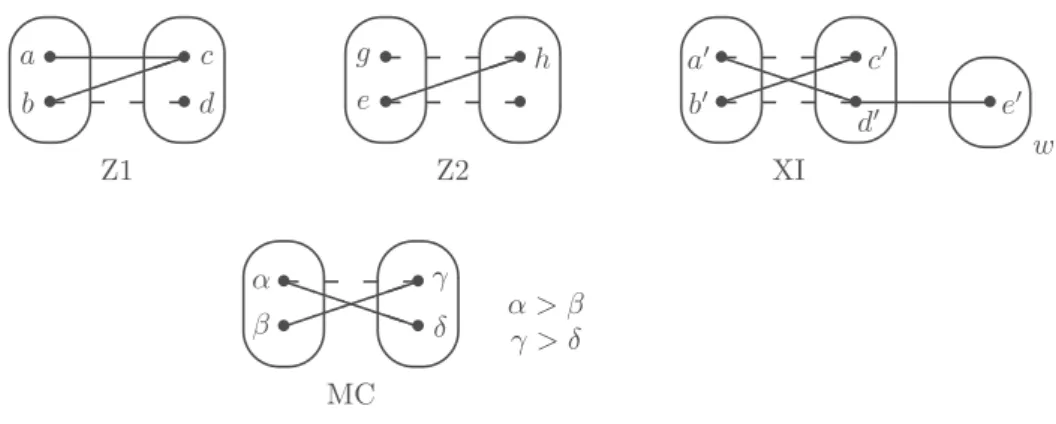
• • • ✏✏✏✏✏ • Z1 ✗ ✖ ✔ ✕ ✗ ✖ ✔ ✕ a b c d • • • ✏✏✏✏✏ • Z2 ✗ ✖ ✔ ✕ ✗ ✖ ✔ ✕ e g h • • • ✏✏✏✏✏ •PPPPP • XI ✗ ✖ ✔ ✕ ✗ ✖ ✔ ✕ ✗ ✖ ✔ ✕ a′ b′ c′ d′ e′ w • • • ✏✏✏✏✏ •PPPPP MC ✗ ✖ ✔ ✕ ✗ ✖ ✔ ✕ α β γ δ α > βγ > δ
Figure 1 Four patterns.
∀i, j ∈ {1, . . . , n} with i Ó= j, ∀p ∈ Ai, ∀q ∈ Aj: {p, q} ∈ E+ ⇒ {f (p), f (q)} ∈ E′+ and
{p, q} ∈ E− ⇒ {f (p), f (q)} ∈ E′−.
Note that forming a homomorphic image of a pattern allows the parts to be renamed, and points p, q within the same part to be merged (provided there is no third point r such that {p, r} and {q, r} are different types of edges).
We will say that a pattern P occurs as a sub-pattern of a pattern Q if Q can be transformed into a homomorphic image of P by a sequence of the following substructure operations:
removal of (positive or negative) edges, removal of isolated points, and
removal of empty parts.
A binary CSP instance is a pattern in which a part Aicorresponds to the set of assignments
to a variable; hence elimination of a part corresponds to the elimination of a variable. Consider the three patterns Z1, Z2 and XI shown in Figure 1. Points are represented by bullets, and points representing assignments to the same variable v are grouped together within an oval representing Av. Solid lines represent positive edges (i.e., compatibility of
the corresponding pair of points) and dashed lines negative (i.e., incompatibility) edges. For example, the pattern Z1 consists of 4 points a, b ∈ Av0, c, d ∈ Av1, two positive edges
E+= {ac, bd} and one negative edge E−= {bd}. Z1 occurs in Z2 since Z2 can be transformed
into a homomorphic image of Z1 by removal of edge gh and point g (under a homomorphism that maps a and b to the same point e in Z2). The pattern Z2 occurs in XI (as a subpattern) since XI can be transformed into a homomorphic image of Z2 by removal of the edges a′d′
and d′e′ followed by the removal of the (then) isolated point e′ together with the (then)
empty part w. By transitivity of the occurrence relation, Z1 also occurs in XI.
We also consider patterns with structure in the sense of relations between the points in a pattern. In this case the homomorphism f in the definition of homomorphic image, above, must preserve the structure of the pattern. This structure may be, for example, an order on the parts (i.e., variables) or an order on points within a part (i.e., domain values). Patterns (such as Z1, Z2 and XI in Figure 1) without any such structure are known as flat patterns [6]. The pattern MC in Figure 1 has the structure consisting of the partial order: α > β, γ > δ. Since XI is a flat pattern, MC does not occur in XI since this partial order clearly cannot be preserved by a homomorphism from MC to XI. On the other hand, Z1 occurs in MC (via a homomorphism which maps both a and b to α, c to δ and d to γ) since Z1 has no structure to be preserved.
A class of binary CSP instances can be defined by forbidding a pattern P . We use the notation CSPSP(P ) to represent the set of binary CSP instances in which the pattern P does
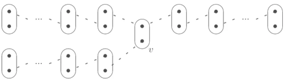
✎ ✍ ☞ ✌ • • ✎ ✍ ☞ ✌ • • ✎ ✍ ☞ ✌ • • ✎ ✍ ☞ ✌ • • ✎ ✍ ☞ ✌ • • ✎ ✍ ☞ ✌ • • ✎ ✍ ☞ ✌ • • ✎ ✍ ☞ ✌ • • ✎ ✍ ☞ ✌ • • ✎ ✍ ☞ ✌ • • ... ... ... v
Figure 2 The negative pattern Pivot(k), where the number of edges in each of the three branches
leaving the central variable v is k.
not occur as a subpattern. We say that a pattern P is tractable if there is a polynomial-time algorithm to solve CSPSP(P ) and intractable if CSPSP(P ) is NP-hard. The pattern MC is tractable since CSPSP(MC) is the class of binary max-closed instances [36]. On the other hand, we know that Z2 is intractable since it does not satisfy a necessary condition for tractability described in Section 3.2. If P occurs as a subpattern of Q, then CSPSP(P ) ⊆ CSPSP(Q) and hence P is tractable if Q is tractable [6]. Thus we can immediately deduce that Z1 is tractable (since it occurs in MC) and that XI is intractable (since Z2 occurs in XI).
An important point is that applying any reduction operation which eliminates domain elements, such as arc consistency, SAC (Singleton Arc Consistency) or neighbourhood substitution [24], cannot introduce a pattern in an instance. On the other hand, reduction operations, such as 3-consistency, which modify constraints may introduce patterns.
A pattern P (such as pattern Z1 in Figure 1) is mergeable if there exists some pattern Q (such as the pattern Z1 without the edge ac or the point a) such that Q is a homomorphic image of P but P is not a homomorphic image of Q; otherwise, P is unmergeable. A point p (such as e′ in pattern XI in Figure 1) is called dangling if p belongs to at most one positive
edge {p, q} and no negative edges (and p belongs to no other relation, such as a partial order, in the case of patterns with structure). The corresponding dangling reduction consists in removing both the edge {p, q} and the point p (together with the part to which p belonged if this part becomes empty after removal of p). Dangling points provide no information in arc-consistent instances, in the sense that P occurs in an instance I if and only if the pattern
P′ occurs in I where P′ is the result of applying a dangling reduction to P . Thus, using the
fact that establishing arc consistency cannot introduce patterns, we have that P is tractable if and only if P′ is tractable.
An unmergeable pattern with no dangling points is called irreducible. In Figure 1, pattern Z1 is mergeable, whereas patterns Z2 and XI are unmergeable. The point e′ in pattern XI is
dangling (as is the point a in the pattern Z1) but not β and δ in pattern MC (because of the partial order relation on these points). Thus of the four patterns in Figure 1, only Z2 and MC are irreducible.
3.2
Characterising Tractable Patterns
The theoretical tools necessary to provide a complete characterisation of tractable patterns have yet to be discovered. Indeed, characterising tractable patterns would appear to be, in general, even more difficult than characterising tractable constraint languages or tractable constraint-hypergraph structures. Nevertheless, certain characterisation results have been proved. One important result concerns the negative edges in a tractable unmergeable pattern. It has been shown that the “skeleton” of a tractable unmergeable pattern, consisting of just
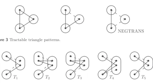
• ◗ ◗ ◗ • ✑✑ ✑• ✓ ✒ ✏ ✑ ✓ ✒ ✏ ✑✓ ✒ ✏ ✑ • • ✑✑ ✑• ✓ ✒ ✏ ✑ ✓ ✒ ✏ ✑✓ ✒ ✏ ✑ • • • NEGTRANS ✓ ✒ ✏ ✑ ✓ ✒ ✏ ✑✓ ✒ ✏ ✑ Figure 3 Tractable triangle patterns.
• • • ✑✑ ✑ • ◗ ◗ ◗ T1 ✓ ✒ ✏ ✑ ✓ ✒ ✏ ✑✓ ✒ ✏ ✑ • • • ✑✑ ✑ • PPP • T2 ✓ ✒ ✏ ✑ ✓ ✒ ✏ ✑ ✓ ✒ ✏ ✑ • • • • PPP • T3 ✓ ✒ ✏ ✑ ✓ ✒ ✏ ✑ ✓ ✒ ✏ ✑ • • • ✑✑ ✑ • ◗ ◗ ◗ • T4 ✓ ✒ ✏ ✑ ✓ ✒ ✏ ✑✓ ✒ ✏ ✑ • • • • ◗ ◗ ◗ T5 ✓ ✒ ✏ ✑ ✓ ✒ ✏ ✑✓ ✒ ✏ ✑ Figure 4 The five tractable irreducible flat patterns on 3 variables and 2 constraints.
the negative edges, must occur as a subpattern of (possibly multiple copies of) the pattern Pivot(k), shown in Figure 2, for some constant k [6]. Unfortunately, very little is known about the positive edges that can be added to such skeletons of negative edges.
Given that a general characterisation seems, for the moment, out of reach, certain special cases have been studied, such as triangle patterns and 2-constraint patterns [19, 15]. Figure 3 shows the three tractable flat patterns on a triangle of 3 points and 3 edges [19]. Although the first two patterns define fairly trivial classes, the third one, called NEGTRANS, is interesting since CSPSP(NEGTRANS) includes non-trivial instances composed of arbitrary unary constraints and non-overlapping All-Different constraints [48, 55]. The class of binary CSP instances satisfying this negative-transitivity property has been generalised to a large tractable class of optimisation problems involving cost functions of arbitrary arity which we will discuss in Section 7 [19]. Figure 4 shows the five tractable irreducible flat patterns on 3 variables and 2 constraints [15]. CSPSP(T4) is interesting since it includes all binary CSP
instances with zero-one-all constraint relations [13] (which can be seen as a generalisation of 2SAT to non-Boolean domains).
Given the relatively modest successes in defining new and useful tractable classes by forbidding flat patterns, it is natural to consider possible extensions of patterns by studying structured patterns, non-binary patterns and other forms of occurrence than subpattern occurrence. These three extensions are the subject of the remainder of this section.
3.3
Partially-Ordered Patterns
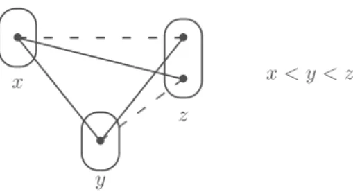
The pattern BTP shown in Figure 5 is known as a broken triangle (since the positive edges can be said to form a triangle which is broken at variable z). Forbidding this pattern on all triples of variables x < y < z defines a tractable class CSPSP(BTP) [16]. This class includes all binary CSP instances whose constraint graph is a tree T since, ordering the variables according to a pre-order of T , each variable z is constrained by at most one variable y < z, its parent in T , and hence the broken-triangle pattern cannot occur. If a variable ordering exists such that the broken-triangle pattern does not occur, then this order can be found in polynomial time: it suffices to establish arc consistency and then successively eliminate variables v which are not the right-hand variable z of a broken triangle (since we know that such a variable v can be the last variable in the ordering among the remaining variables).
✎ ✍ ☞ ✌ • ✎ ✍ ☞ ✌ • ✎ ✍ ☞ ✌ • • ❳❳❳❳ ❳❳❳❳ ❭ ❭ ❭ ❭ ❭✜✜ ✜✜ ✜ x y z x < y < z
Figure 5 A binary CSP instance satisfies the broken triangle property if this pattern (known as
a broken triangle or BTP) does not occur in the instance.
CSPSP(BTP) is solved by arc consistency since the BTP is exactly the obstruction which prevents an arc-consistent instance being backtrack-free. Indeed, even if the variable order is unknown, MAC (Maintaining Arc Consistency) solves CSPSP(BTP) [16]. Thus, most CSP solvers will automatically solve in polynomial time all instances in CSPSP(BTP).
◮Example 1. Consider a company which wishes to give bonuses to its n employees. Each
employee i ∈ {1, . . . , n} has a grade gradei, with higher grades corresponding to more
important posts. Some, but not all, employees have an immediate boss to whom they report. The company wants to assign bonuses so that each employee’s bonus is a multiple of 50 euros between 5% and 20% of their salary. If an employee i has an immediate boss bi, then the
sum of the bonuses of i and bimust be no less than 10% and no more than 30% of the salary
of bi. On the other hand, if an employee i has no immediate boss then the rule is that they
must not receive a bigger bonus than anyone at a higher grade.
Let the variable xi be the bonus assigned to employee i. We assume that employees are
numbered so that (gradei> gradej) ⇒ (i < j). Thus, for example, employee number 1 is
the CEO of the company. The domain of xi is the multiples of 50 between 5% and 20% of
the salary sali of employee i. If employee i has a boss bi, then there is a binary constraint
0.1salbi ≤ xi+ xbi ≤ 0.3salbi. Indeed, this is the only constraint between xiand the variables
xj (j < i). If employee i has no boss, then there are binary constraints xi ≤ xj for each
j ∈ {1, . . . , i − 1} such that gradej > gradei. In either case, it is easy to verify that xi
cannot be the rightmost variable in the broken triangle pattern shown in Figure 5. Thus, this problem falls in CSPSP(BTP) and is solved by arc consistency. The constraint graph is of unbounded tree-width: for example, if no-one has a boss but everyone is at a different grade, then the constraint graph is the complete graph. Furthermore, the language of constraints is NP-hard. Thus, this bonus-assignment problem defines a truly hybrid tractable class.
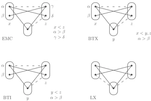
We have seen that broken-triangle free instances are solved by arc consistency. Arc consistency is also a decision procedure for CSPSP(EMC) where EMC (Extended Max-Closed) is the pattern shown in the top left of Figure 6. EMC is particularly interesting because CSPSP(EMC) is a strict generalisation of binary max-closed CSPs [36] (since the pattern MC shown in Figure 1 is a subpattern of EMC).
◮Example 2. Consider a binary CSP instance I with integer domains and in which all
binary constraints are of the following form:
aXi+ bXj ≥ c
where a, b, c are non-zero constants. We say that Xioccurs positively (respectively, negatively)
✎ ✍ ☞ ✌ • • ✎ ✍ ☞ ✌ • ✎ ✍ ☞ ✌ • • ❳❳❳❳ ❳❳❳❳ ✘✘✘✘✘✘ ✘✘ ❭ ❭ ❭ ❭ ❭✜✜ ✜✜ ✜ x z x < z α > β γ > δ α β γ δ EMC ✎ ✍ ☞ ✌ • • ✎ ✍ ☞ ✌ • ✎ ✍ ☞ ✌ • • ❳❳❳❳ ❳❳❳❳ ✘✘✘✘✘✘ ✘✘ ❭ ❭ ❭ ❭ ❭✜✜ ✜✜ ✜ y x z x < y, z α > β α β BTX ✎ ✍ ☞ ✌ • • ✎ ✍ ☞ ✌ • ✎ ✍ ☞ ✌ • • ❳❳❳❳ ❳❳❳❳ ✘✘✘✘✘✘ ✘✘ ❭ ❭ ❭ ❭ ❭✜✜ ✜✜ ✜ y z y < z α > β α β BTI ✎ ✍ ☞ ✌ • • ✎ ✍ ☞ ✌ • ✎ ✍ ☞ ✌ • • ❳❳❳❳ ❳❳❳❳ ✘✘✘✘✘✘ ✘✘ ❭ ❭ ❭ ❭ ❭✜✜ ✜✜ ✜ LX
Figure 6 Partially-ordered patterns that are solved by arc consistency.
Xi, Xj occurs positively [36]. Suppose that in I, for all constraints on a pair of variables
Xi< Xj in which both variables occur negatively, the variable Xj only occurs negatively in
other constraints. Then I ∈ CSPSP(EMC), and hence is solved by arc consistency.
In fact, if we consider only unmergeable patterns to which we then add a partial order to the variables and/or the domains, then there are just five patterns P such that arc consistency is a decision procedure for CSPSP(P ): BTP and the patterns EMC, BTX, BTI and LX shown in Figure 6 [20]. Given a fixed total order of the domain, there is a polynomial-time algorithm to find a total variable ordering such that any one of these patterns does not occur in an instance (or to determine that no such ordering exists). However, if the domain and variable orders are both unknown, then EMC, BTX and BTI become NP-complete to detect [20].
3.4
Non-Binary CSPs
Most work on forbidden-pattern tractability has been restricted to binary CSPs. Indeed, notions such as microstructure and forbidden pattern do not (yet) have a widely-accepted generalisation to non-binary constraints. Nonetheless, the notion of arbitrary-arity patterns can be said to be already present in language classes defined by a polymorphism [11]. A polymorphism can be viewed as a forbidden pattern in each constraint relation R of the instance. The forbidden pattern corresponding to a polymorphism f : Dr → D consists
of a set of r positive tuples and one negative tuple. The positive tuples t1, . . . , tr ∈ R
are consistent assignments to the same variables and the negative tuple f(t1, . . . , tr) /∈ R
is the assignment to the same variables resulting from the pointwise application of f to the t1, . . . , tr. By forbidding the pattern (t1, . . . , tr∈ R, f (t1, . . . , tr) /∈ R), we impose the
well-known polymorphism condition t1, . . . , tr∈ R =⇒ f (t1, . . . , tr) ∈ R [11].
As we have seen in Section 3.3, in the binary CSP, the broken-triangle property defines a tractable class CSPSP(BTP). Although the definition of tractable classes by forbidden
✎ ✍ ☞ ✌ • ✎ ✍ ☞ ✌ • ✎ ✍ ☞ ✌ • • ❤❤❤❤❤❤ ❆ ❆ ❆ ❆✜✜ z ✜✜ ✜ a b t<z X Y u<z
Figure 7 Illustration of a directional general-arity broken triangle.
patterns in general-arity CSPs is an area which remains largely unexplored, a generalisation of the broken-triangle class CSPSP(BTP) to general-arity CSPs has recently been given [14].
Purely for notational convenience we assume that a CSP instance I is given in the form of a set of negative (incompatible) tuples NoGoods(I), where a tuple is a set of variable-value assignments, and that the predicate Good(I, t) is true iff the tuple t does not contain any pair of distinct assignments to the same variable and ∄t′⊆ t such that t′ ∈ NoGoods(I). We
write Good as a predicate whereas Nogoods(I) is a set to emphasize the asymmetry between the notions of positive and negative tuples. This asymmetry is not evident in the case of binary CSPs nor in the case of polymorphisms.
We suppose that a total ordering < of the variables of a CSP instance I is given. We write
t<x to represent the subset of the tuple t consisting of assignments to variables occurring
before x in the order <, and V ars(t) to denote the set of all variables assigned by t. ◮Definition 3. A directional general-arity broken triangle (DGABTP) on assignments a, b to variable z in a CSP instance I is a pair of tuples t, u (containing no assignments to variable
z) satisfying the following conditions:
1. t<z and u<z are non-empty,
2. Good(I, t<z∪ u<z) ∧ Good(I, t<z∪ {éz, aê}) ∧ Good(I, u<z∪ {éz, bê}),
3. t ∪ {éz, bê} ∈ NoGoods(I) ∧ u ∪ {éz, aê} ∈ NoGoods(I),
4. ∃t′ s.t. V ars(t′) = V ars(t) ∧ (t′)<z= t<z ∧ t′∪ {éz, aê} /∈ NoGoods(I),
5. ∃u′ s.t. V ars(u′) = V ars(u) ∧ (u′)<z= u<z ∧ u′∪ {éz, bê} /∈ NoGoods(I). I satisfies the directional general-arity broken-triangle property (DGABTP) according to the variable ordering < if no directional general-arity broken triangle occurs on any pair of values
a, b for any variable z.
Points (1), (2) and (3) of Definition 3 are illustrated by Figure 7. This figure is similar to Figure 5 except that X,Y are sets of variables and t<z,u<z are tuples. Note that the sets
X = V ars(u<z) and Y = V ars(t<z) may overlap. Solid lines now represent partial solutions
(i.e., consistent assignments to subsets of variables). The two dashed lines represent nogoods (i.e., tuples not in the constraint relation on its variables) u ∪ {éz, aê} and t ∪ {éz, bê} which possibly involve assignments to variables w > z. In the case of binary CSPs, a directional general-arity broken triangle is equivalent to a broken triangle as shown in Figure 5 (since nogoods, being binary, involve no other variables w > z and the sets X, Y are necessarily singletons). Points (4) and (5) of Definition 3 are technical conditions (which always hold if a weak form of directional consistency holds) ensuring that the DGABTP can be tested in polynomial time for a given order whether constraints are given as tables of satisfying assignments or as nogoods.
Any instance I satisfying the DGABTP can be solved in polynomial time by repeatedly applying the following two operations: (i) merge two values in the last remaining variable
(according to the order <); (ii) eliminate this variable when its domain becomes a singleton.
Merging values a, b ∈ D(z) in a general-arity CSP instance I consists of replacing a, b in D(z)
by a new value c which is compatible with all variable-value assignments compatible with at least one of the assignments éz, aê or éz, bê, thus producing an instance I′ with the new set
of nogoods defined as follows:
NoGoods(I′) = {t ∈ NoGoods(I) | éz, aê, éz, bê /∈ t} ∪ {t ∪ {éz, cê} | t ∪ {éz, aê} ∈ NoGoods(I) ∧
∃t′∈ NoGoods(I) s.t. t′ ⊆ t ∪ {éz, bê}} ∪ {t ∪ {éz, cê} | t ∪ {éz, bê} ∈ NoGoods(I) ∧ ∃t′∈ NoGoods(I) s.t. t′ ⊆ t ∪ {éz, aê}} .
In general, merging a pair of values in an instance I may produce an instance I′ which is
satisfiable even though I was not, but forbidding directional general-arity broken triangles prevents this from happening. Eliminating a variable z whose domain is a singleton {a} consists in making the assignment éz, aê and eliminating éz, aê from all nogoods.
Unfortunately, when the variable order is not given, testing the existence of a variable ordering for which a CSP instance satisfies the DGABTP is NP-complete in the general-arity case [14]. This can be contrasted with the binary case in which this test is polytime.
Note that the set of general-arity CSP instances whose dual instance satisfies the BTP, denoted by DBTP, also defines a tractable class which can be recognised in polynomial time even if the ordering of the variables in the dual instance is unknown [44]. This DBTP class is incomparable with DGABTP (which is equivalent to BTP in binary CSP) since DBTP is known to be incomparable with the BTP class already in the special case of binary CSP [44]. A general-arity broken triangle can be said to be centred on a pair of values in the domain of a variable whereas a broken triangle in the dual instance is centred on a pair of tuples in a constraint relation. One consequence of this is that eliminating tuples from constraint relations cannot introduce broken triangles in the dual instance, whereas the DGABTP is only invariant under elimination of domain values. On the other hand, the DGABTP is invariant under adding a complete constraint (i.e., whose relation is the direct product of the domains of the variables in its scope) whereas this operation can introduce broken triangles in the dual instance. Another important difference is that DGABTP depends on an order on the variables whereas DBTP depends on an order on the constraints.
The generalisation of forbidden patterns to non-binary constraints is a largely unexplored area of research, but the generalisation of BTP to DGABTP has highlighted the asymmetry between positive and negative tuples when constraints are non-binary.
3.5
Quantified Patterns
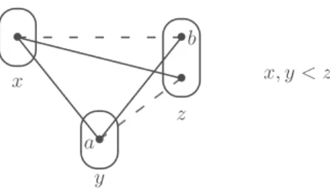
The notion of forbidding patterns has also been extended to rules based on applying a sequence of quantifiers to the variables and values in a pattern. This has led to the discovery of novel variable-elimination or value-elimination techniques [7, 12]. As an example, consider the broken triangle pattern shown in Figure 5. It is known that we can eliminate variables which are not the right-hand variable of a broken triangle: the resulting instance is satisfiable if and only if the original instance was satisfiable [16]. This variable-elimination rule can be strictly generalised to the following rule illustrated in Figure 8: a variable z can be eliminated from an instance I without changing the satisfiability of I if for all other variables
y, ∀a ∈ D(y), ∃b ∈ D(z) with ab a positive edge in I such that no broken triangle exists
✎ ✍ ☞ ✌ • ✎ ✍ ☞ ✌ • ✎ ✍ ☞ ✌ • • ❳❳❳❳ ❳❳❳❳ ❭ ❭ ❭ ❭ ❭✜✜ ✜✜ ✜ x y z x, y < z a b
Figure 8 In the ∀∃BTP class, for all pairs of variables y < z, ∀a ∈ D(y), ∃b ∈ D(z) such that for
all variables x < z, the broken triangle pattern shown does not occur.
such that all variables can be eliminated according to this rule strictly generalises the tractable class CSPSP(BTP), since the BTP imposes the same condition but for all b ∈ D(Xk).
Let I be a binary arc-consistent CSP instance in the ∀∃BTP class and let s be a solution to the instance obtained by eliminating the last variable z from I. We will give a sketch proof that s can be extended to a solution for I. (We refer the reader to [12] for full details.) By assumption, ∀y ∈ X \ {z}, ∀a ∈ D(y), ∃by
a ∈ D(z) with abya a positive edge such that
∀x ∈ X \ {y, z}, ∀c ∈ D(x) with ac a positive edge and by
ac a negative edge, ∀d ∈ D(z) with
cd a positive edge, ad is also a positive edge. For v ∈ X \ {z}, let Im(v) := {d ∈ D(z) | s(v)d
a positive edge}, where s(v) is the value assigned to variable v by s. If x, y ∈ X \ {z} are such that s(x)by
s(y)is a negative edge, then the ∀∃BTP property implies that Im(x) (
Im(y) [12]. Now choose some y ∈ X \ {z} such that Im(y) is minimal for inclusion among the sets Im(v) (v ∈ X \ {z}). Then the assignment éz, by
s(y)ê is compatible with all the
assignments s(x) (x ∈ X \ {y, z}), otherwise we would have Im(x) ( Im(y) (contradicting the minimality of Im(y)). Therefore, s can be extended to a solution to I, by making the assignment s(z) = bs(y).
3.6
Topological Minor Patterns
We now present a new operation on patterns which allows us to define the notion of a topological minor of a pattern (and hence of a binary CSP instance). This new operation is analogous to the operation of eliminating subdivisions (vertices of degree 2) that is used to define a topological minor of a graph [25]. However, since patterns contain two kinds of edges, the definition is slightly more complicated.
This new operation, path reduction, will sometimes lead to the introduction of edges in
E+∩ E− in a coloured microstructure éA1, . . . , A
n, E+, E−ê. This is why we do not impose
the restriction that E+ and E− be disjoint in a pattern.
In a pattern P = éA1, . . . , An, E+, E−ê, we say that two parts Ai, Ajare directly connected
if there is at least one (positive or negative) edge {p, q} ∈ E+∪ E− with p ∈ A
i and q ∈ Aj.
If Ai, Aj are not directly connected and Ak is directly connected only to Ai and Aj, then
the following operation can be performed, which is known as path reduction:
1. ∀p ∈ Ai, ∀q ∈ Aj: if ∃r ∈ Ak such that {p, r}, {r, q} ∈ E+, then introduce a new positive
edge {p, q},
2. ∀p ∈ Ai, ∀q ∈ Aj: if ∃r, s ∈ Ak such that {p, r}, {s, q} ∈ E−, then introduce a new
negative edge {p, q},
3. remove the part Ak and all edges containing points in Ak.
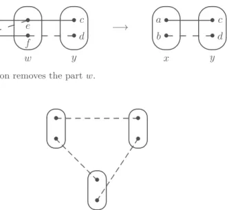
This operation is illustrated in Figure 9. Positive and negative edges are treated differently in this definition; this is because for p ∈ Ai and q ∈ Aj to be part of a solution to the
• • • • • • ✗ ✖ ✔ ✕ ✗ ✖ ✔ ✕ ✗ ✖ ✔ ✕ w x y a b e f c d −→ • • • • ✗ ✖ ✔ ✕ ✗ ✖ ✔ ✕ x y a b c d
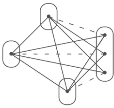
Figure 9 Path reduction removes the part w. ✎ ✍ ☞ ✌ • • ✎ ✍ ☞ ✌ • • ✎ ✍ ☞ ✌ • •
Figure 10 A pattern which defines the class of acyclic binary CSP instances when forbidden as a
topological minor.
sub-instance on variables Xi, Xj, Xk, the points p and q must both be compatible with some
common point r ∈ Ak, whereas p and q may be incompatible if they are each incompatible
with some point in Ak, not necessarily the same point. In Figure 9, after the path reduction
operation which eliminates w, we have a positive edge ac (thanks to the edges ae and ec), but no positive edge bc. We also have a negative edge bd (thanks to the edges be and fd). As in the case of non-binary patterns (c.f. Section 3.4), it is essential to introduce an asymmetry between positive and negative edges in order to obtain a useful notion.
A pattern P occurs as a topological minor of a pattern Q if Q can be transformed into a homomorphic image of P by a sequence of substructure operations (listed above in Section 3.1) and path reductions.
We use the notation CSPTM(P ) to represent the set of binary CSP instances in which the pattern P does not occur as a topological minor. For each pattern P there are therefore two distinct notions of tractability: a pattern P is sub-pattern tractable if there is a polynomial-time algorithm to solve CSPSP(P ); a pattern P is topological-minor tractable if there is a polynomial-time algorithm to solve CSPTM(P ). A pattern which is sub-pattern tractable is topological-minor tractable since any pattern that occurs as a sub-pattern will also occur as a topological minor.
One important tractable class of binary CSP instances is the class of instances whose constraint graph is acyclic [28]. However, this class cannot be defined by a finite set of forbidden sub-patterns [9]. On the other hand, it is straightforward to characterise the class of acyclic instances by forbidding a single pattern as a topological minor. Forbidding the pattern shown in Figure 10 as a topological minor exactly defines the class of binary CSP instances whose constraint graph is acyclic. Indeed, this idea can easily be extended to any of the tractable classes of binary CSP instances defined by imposing any fixed bound on the treewidth of the constraint graph [29] using the graph minor theorem [49]. However, it remains to be seen whether the notion of patterns occurring as topological minors can be used to define a practically useful and genuinely novel tractable class.
4
Classes Requiring a Level of Consistency
Some hybrid tractable classes have been defined which guarantee global consistency if some local property holds after establishing a certain level of local consistency. One example is that the constraints can be decomposed into the join of arity-r constraints after establishing strong d(r − 1) + 1 consistency, where d is the maximum domain size [23]. Of course, in general, establishing this level of consistency introduces constraints of order d(r − 1), so the assumption that constraints are of arity r is very strong. This class has been generalised to the class of arity-r CSP instances which are strongly ((m + 1)(r − 1) + 1)-consistent, where given an r-ary constraint and an instantiation of r − 1 of the variables that participate in the constraint, the parameter m (called the tightness) is an upper bound on the number of instantiations of the rth variable that satisfy the constraint in the case that this is not the whole domain [54].
Naanaa [46] has proposed a generalisation of m-tightness. Let E be a finite set and let {Ei}i∈I be a finite family of subsets of E. The family {Ei}i∈I is said to be independent if
and only if for all J ( I, Ü i∈I Ei ( Ü j∈J Ej.
In particular, observe that {Ei}i∈I cannot be independent if ∃j Ó= j′∈ I such that Ej ⊆ Ej′,
since in this case and with J = I \ {j′} we would have
Ü i∈I Ei = Ü j∈J Ej.
Let I be a CSP instance whose variables are totally ordered by <. Let éσ, Rê be an r-ary constraint whose scope σ contains a variable x and let t be a tuple that instantiates the r − 1 remaining variables of σ. Denote by Rx(t) the set of values in D(x) that can extend t to form
a tuple in the relation R. The directional extension of tuple t to variable x w.r.t. R and < is defined to be Rx(t) if x is the last (w.r.t. the order <) variable in σ, and D(x) otherwise. A
family of extensions of tuples t ∈ T is said to be consistent if and only if the tuple formed by the join ⊲⊳t∈T t of the corresponding tuples is consistent. With respect to the ordering <,
the directional rank of x in I is the size of the largest independent and consistent family of directional extensions to x, and the directional rank κ of I is the maximum directional rank over all its variables. If I is a CSP instance with constraints of arity no greater than r which has directional rank no greater than κ and is directional strong (κ(r − 1) + 1)-consistent, then I is globally consistent [46]. In general, establishing this level of consistency introduces constraints of arity κ(r − 1) which is no greater than r only if κ = 1 or (κ = 2 ∧ r = 2).
There is an interesting link between directional rank and forbidden patterns. Directional rank 1 is equivalent to the broken triangle property (i.e., forbidding as a subpattern the pattern shown in Figure 5) and directional rank κ > 1 subsumes an extension of the broken triangle property known as (κ + 1)-BTP [17]. A binary CSP instance satisfies k-BTP if for all variables z and for all sets S of k variables occurring before z in the variable ordering, ∃x, y ∈ S such that there are no broken triangles on variables x, y, z. We can see that 2-BTP corresponds exactly to the broken triangle property. If a binary CSP instance satisfies 3-BTP after establishment of directional strong 3-consistency, then it has directional rank κ = 2 and is directional strong (κ(r − 1) + 1)-consistent (since r = 2), and hence is globally consistent [46]. Directional rank 2 strictly subsumes 3-BTP since it is equivalent to forbidding (as a subpattern) the pattern shown in Figure 11. This is a natural generalisation
✎ ✍ ☞ ✌ • ✎ ✍ ☞ ✌ • ✎ ✍ ☞ ✌ • • • • ✎ ✍ ☞ ✌ ✥✥✥✥✥✥ ✥✥✥✥ ❵❵❵❵❵ ❵❵❵❵❵ ◗ ◗ ◗ ◗ ◗ ◗ ◗ ◗ ◗ ◗ ◗ ◗ ❅ ❅ ❅ ❅ ❅ ❅ ❈ ❈ ❈ ❈ ❈ ❈ ❈ ❈✡✡ ✡✡ ✡✡✡
Figure 11 A binary CSP instance has directional rank 2 if this pattern does not occur in the
instance.
of the broken-triangle pattern shown in Figure 5, but, unfortunately, we also require strong directional 3-consistency to obtain a tractable class and establishing this level of consistency may introduce the pattern.
5
Microstructure-Based Classes
We recall the definition of microstructure. We have seen that a binary CSP instance on variables X1, . . . , Xn can be represented by the domain D(Xi) of each variable Xi and a
binary relation Rijfor each pair of variables Xi, Xj(i Ó= j) consisting of all possible consistent
assignments to this pair of variables. If I is a binary CSP instance, then its microstructure is a graph éA, Eê where A = {(Xi, a) | a ∈ D(Xi)} is the set of possible variable-value
assignments and E = {{(Xi, a), (Xj, b)} | (a, b) ∈ Rij} [37]. The microstructure relies on
both the structure and the relations of the instance I and so is a natural place to look for hybrid tractable classes. In this section we study properties of the graph éA, Eê in which A is not partitioned into parts corresponding to variables (as was the case in patterns, studied in Section 3). Ignoring variable information has the obvious disadvantage that we lose possibly valuable information, but has the advantage that deep theorems from graph theory can be directly applied.
The complement of a graph G = éV, Eê is the graph with vertices V and whose edges are the non-edges of G. The microstructure complement is the complement of the microstructure. Solutions to I are in one-to-one correspondence with the n-cliques of the microstructure of I and with the size-n independent sets of the microstructure complement of I.
The chromatic number of a graph is the smallest number of colours required to colour its vertices so that no two adjacent vertices have the same colour. A graph G is perfect if for every induced subgraph H of G, the chromatic number of H is equal to the size of the largest clique contained in H. Since a maximum clique in a perfect graph can be found in polynomial time [33], the class of binary CSP instances with a perfect microstructure is tractable as a direct consequence, as observed in [50]. Perfect graphs can also be recognized in polynomial time [3].
For a class of graphs C, a graph G is C-free if no induced subgraph of G is isomorphic to any graph in C. The cycle of order k is the graph with vertices v1, . . . , vk and edges {vk, v1}
and {vi, vi+1} for i = 1, . . . , k − 1. A hole is a cycle of length k ≥ 5. An antihole is the
complement of a hole. An alternative definition of perfect graphs is that a graph is perfect if and only if it is (odd-hole,odd-antihole)-free [4]. Chordal graphs are examples of perfect graphs. Interesting examples of binary CSP instances whose microstructure is perfect are
instances with unary constraints together with a global AllDifferent constraint [50], instances which are arc consistent and max-closed after independent (and possibly unknown) permutations of each domain [31].
6
Weakly or Strongly Constrained Instances
One way to define a tractable class is to only allow a small number of weak constraints, in order to guarantee that the instance is always satisfiable. For example, if each variable is in the scope of at most t constraints and in each constraint relation the proportion of tuples that are disallowed is strictly less than 1/e(r(t − 1) + 1), where e is the base of natural logarithms and r the arity of the constraint, then the instance is necessarily satisfiable [47].
Another way to define a tractable class is to consider only instances which are sufficiently strongly constrained so that there is necessarily only a small number of partial solutions examined during search (and hence a small number of solutions). A simple example of a condition that guarantees a polynomial number of solutions is functionality. A constraint éσ, Rê is functional on variable Xi∈ σ if the relation R contains no two assignments differing
only at variable Xi. A CSP instance is functional with root set of size k if there exists
a variable ordering X1 < . . . < Xn such that, for all i ∈ {k + 1, . . . , n}, there is some
constraint éσ, Rê with Xi ∈ σ ⊆ {X1, . . . , Xi} that is functional on Xi. (Note that this
implies tractability.) In the case of binary CSP instances, a minimum root set can be found in polynomial time [22]. Unfortunately, determining the size of a minimum root set is NP-hard for ternary CSP instances [8].
Another condition that guarantees a backtracking search tree of polynomial size (assuming domain size bounded by a constant) is the k-Turan property [8] which we now define. Indeed, this property is very strong since it guarantees a polynomial-size search tree for all variable orderings. We say that a subset of variables S represents another set T if S ⊆ T . An (n, k)-Turan system is a pair éX, Bê where B is a collection of subsets of the n-element set
X such that every k-element subset of X is represented by some set in B. For example, let
C4Turan be the class of binary CSP instances over a set of variables X, each with a Boolean
domain, in which each constraint is equivalent to a 3SAT clause and for each quadruple of distinct variables Xi, Xj, Xk, Xℓ there is at least one ternary constraint whose scope is a
subset of these variables. In this example, every 4-element subset of the set of n variables X is represented by the scope of some ternary constraint, and hence éX, Sê, where S is the set of constraint scopes, is an (n, 4)-Turan system. An n-variable CSP instance over domain D and variables X is k-Turan if éX, Bê forms an (n, k)-Turan system where B is the set of the scopes of the constraints éσ, Rê for which
∀a, b ∈ D, {a, b}|σ|* R .
This condition says that at least one tuple is disallowed by the constraint over each Boolean subdomain {a, b} of D. In the class C4Turan, all constraints satisfy this condition and hence
C4Turan is tractable since all instances in this class satisfy the 4-Turan property. Generalising
this example, the class of k-SAT instances where every k′-tuple of variables, where k′≥ k, is
restricted by a clause is k′-Turan and hence tractable.
It is an open question whether the k-Turan property can be relaxed in a way that guarantees a polynomial-size search tree for just one variable ordering, rather than all variable orderings, while imposing a weaker condition than functionality.
7
Valued CSPs
CSPs are inherently decision problems. In this section we discuss hybrid classes of valued CSPs, which is a generalisation of CSPs to problem that capture both decision and optimisation problems (and their combinations).
We denote by Q = Q ∪ {∞} the set of extended rationals. A valued constraint satisfaction
problem (VCSP) instance I is given by a triple éX, D, Cê, where X = {X1, . . . , Xn} is a finite
set of variables, D is a finite set of values, and C : Dn→Q is an objective function expressed
as a sum of valued constraints, i.e., C(X1, . . . , Xn) =
i=1γi(vi), where γi : Dki →Q is
a cost function of arity ki and vi ∈ Xki is the scope of the valued constraint γi(vi). The
question is to find an assignment of values to the variables that minimises the objective function C.
The class of VCSP instances with {0, ∞}-valued cost functions corresponds to the class of CSP instances. VCSP instances with {0, 1}-valued cost functions are known as Min-CSPs. VCSP instances with Q-valued cost functions are known as finite-valued CSPs [53].
Similarly to the case of CSPs, language-restricted VCSPs parameterised by the set of allowed cost functions in the instance have been studied [42]. In this section we will mention known results on the complexity of hybrid classes of VCSPs.
The idea of lifted languages briefly discussed in Section 2.3 has also been applied to certain VCSPs [39, 52].
7.1
JWP and Generalisations
The study of hybrid classes of VCSPs was initiated in [18], where an interesting hybrid class called the joint winner property (JWP) was discovered. A class of binary VCSPs satisfies the JWP if for any three variable-value assignments (to three distinct variables), the multiset of pairwise costs imposed by the binary valued constraints does not have a unique minimum. If there is no valued constraint with the scope, say, v = éXi, Xjê, then we view it as a 0-valued
constraint γ(v), where γ : D2→Q is the constant-0 binary cost function. Note that the
unary valued constraints in a VCSP that satisfies the JWP can be arbitrary. JWP generalises the tractable pattern NEGTRANS discussed in Section 3.2, as the NEGTRANS pattern precisely forbids the combination of one 0 cost and two ∞ costs.
Following the discovery of JWP, Cooper and Živný classified classes of binary CSPs, Min-CSPs, finite-valued CSPs, and VCSPs parametrised by the allowed types of costs in triples of variable-value assignments (called triangles) [19]. In all studied cases, JWP was essentially the only interesting tractable case. Moreover, [19] generalised JWP to the tractable class of VCSPs with the cross-free convex (CFC) property.
A function g : {0, . . . , s} → Q is called convex on the interval [l, u] if g is Q-valued on the interval [l, u] and the derivative of g is nondecreasing on [l, u], that is, g(m + 2) − g(m + 1) ≥
g(m + 1) − g(m) for all m = l, . . . , u − 2.
Sets A1, . . . , Ar⊆ A are called cross-free if for all 1 ≤ i, j ≤ r, either Ai⊆ Aj, or Ai⊇ Aj,
or Ai∩ Aj= ∅, or Ai∪ Aj= A [51].
We interpret a solution s : X → D to a VCSP instance I = éX, D, Cê as its set of variable-value assignments {éXi, s(Xi)ê | i = 1, . . . , n}. If Aiis a set of variable-value assignments of
a VCSP instance I and s a solution to I, then we use the notation |s ∩ Ai| to represent the
number of variable-value assignments in the solution s that lie in Ai.
Finally we have everything we need to define the CFC property. Let I be a VCSP instance. Let A1, . . . , Ar be cross-free sets of variable-value assignments of I. Let si be the number
property if the objective function of I is g(s) = g1(|s ∩ A1|) + . . . + gr(|s ∩ Ar|), where each
gi : [0, si] → Q (i = 1, . . . , r) is convex on an interval [li, ui] ⊆ [0, si] and gi(z) = ∞ for
z ∈ [0, li− 1] ∪ [ui+ 1, si].
We remark that the functions gi above are not the cost functions associated with the
valued constraints. Note that similarly to JWP, the addition of any unary cost function cannot destroy the cross-free convexity property because for each variable-value assignment éXi, aê we can add the singleton Ai= {éXi, aê}, which is necessarily either disjoint from or
a subset of any other set Aj (and furthermore the corresponding function gi: {0, 1} →Q is
trivially convex).
A special case of the CFC property are global cardinality constraints [48, 56] on cross-free sets.
◮Example 4. To give a concrete example, consider a company which needs to assign staff to a project, minimising total salary cost while respecting constraints concerning the minimum number of personnel from each section, the maximum total number of staff on the project, as well as the availability of each member of staff. We can code this as a VCSP with a boolean variable Xifor each member of staff with Xiassigned the value true if the person in
question is assigned to the project. The availability of each member of staff, as well as his/her salary, can be coded as a unary cost function. Assuming each member of staff belongs to a single section of the company, the remaining constraints are global cardinality constraints on cross-free sets.
The employees, numbered from 1 to n, are partitioned into sections Sj (j = 1, . . . , t).
Let Aj = {éXi, trueê | i ∈ Sj} (j = 1, . . . , t), A0 = ttj=1Aj, and At+i = {éXi, trueê}
(i = 1, . . . , n). The sets Ai (i = 0, . . . , t + n) are cross-free. Let g≤m : {0, . . . , n} →Q be
the function given by g≤m(x) = 0 if x ≤ m and g≤m(x) = ∞ if x > m, with g≥m defined
similarly. For i = 1, . . . , n, let hi: {0, 1} →Q be the function given by hi(0) = 0 and hi(1)
equal to the salary of employee i if he/she is available to work on the project, ∞ if not. Suppose that the project requires at least ni employees from section i, for each i = 1, . . . , t,
making a total of at most N staff members. Then the objective function is
g≤N(|s ∩ A0|) + t Ø j=1 g≥ni(|s ∩ Aj|) + n Ø i=1 hi(|s ∩ At+i|) .
The functions g≤N and g≥ni are convex (indeed constant) on the interval on which they are finite, and each hi is trivially convex on the interval [0, 1].
It has recently been shown1 that the class of convex cross-free VCSPs is a special case of
M♯-convex functions studied in [45] and that JWP precisely captures binary M♯-completable
functions.
7.2
Planarity
Similarly to the planar CSPs discussed in Section 2.1, one can define planar VCSPs. Fulla and Živný gave necessary conditions on the tractability of planar VCSPs [30]. In particular, they showed that if Γ is a Boolean valued constraint language such that VCSP(Γ) is intractable then VCSPp(Γ) is intractable unless Γ is self-complementary in the valued sense; i.e., for every
γ ∈ Γ and every tuple t, γ(t) = γ(t). This is a generalisation of the self-complementarity