Measures in Mamba

HAL Id: hal-00879624

https://hal.archives-ouvertes.fr/hal-00879624

HAL is a multi-disciplinary open access archive for the deposit and dissemination of sci-entific research documents, whether they are pub-lished or not. The documents may come from teaching and research institutions in France or abroad, or from public or private research centers.

L’archive ouverte pluridisciplinaire HAL, est destinée au dépôt et à la diffusion de documents scientifiques de niveau recherche, publiés ou non, émanant des établissements d’enseignement et de recherche français ou étrangers, des laboratoires publics ou privés.

Measures in Mamba

Serge Beucher

To cite this version:

Measures in Mamba

Serge Beucher

CMM/ARMINES

http://www.mamba-image.org

This short note aims at explaining how some measures are implemented in the Mamba software library (module measure.py). For a more detailed introduction to these measures and, more generally, to stereology, refer to [2].

1. General information

• All the measures are performed on binary images (remind that the only built-in measure

which applies on 1-bit, greyscale or 32-bit images is computeVolume).

• All the dimensional measures, that is measures related to a length (1-dimensional) or an area (2-dimensional) use a scale factor. This scale factor is explained below. These measures return real values.

• Non dimensional measures return integer values.

• These measures can be performed on both grids (hexagonal or square). We tried to maintain a strong similarity between the results of the measures performed on one grid or the other (it is the case for instance for the area) but similarity does not mean identity! It is perfectly normal that a perimeter measured with an hexagonal grid be not equal to the same measure performed on a square grid. It is also normal that non dimensional measures (number of components for instance) be different.

2. Scale factor

The scale factor s is a vector (a tuple in Mamba) indicating the horizontal and verical scale factors of the image to be measured (Figure 1):

scale_factor = (sh, sv)

sh indicates the distance between two adjacent pixels of an horizontal line of the image. This value

is supposed to be constant in the whole image (which, in practice, may not be the case, due to image distortions for instance).

sv is the distance between two successive horizontal lines of the image (here again, it is assumed to

be constant).

These two values are real numbers and they are set to 1.0 by default. You can obviously change these values if you know (after a calibration for example) which real values these parameters correspond to.

Figure1: Scale factor on square and hexagonal grids

Note that, on hexagonal grid, setting the scale factor to the default value means that you are not using an isotropic hexagonal grid (where all the triangles would be equilateral).

3. Area

The area is simply computed by multiplying the number of pixels in the binary image (provided by computeVolume) with the area of the influence box surrounding each pixel (Figure 2):

area = sh . sv . number_of_pixels

Figure 2: Influence box of each pixel in square and hexagonal grids

This area is the same whatever the chosen grid.

4. Diameter (diametral variation)

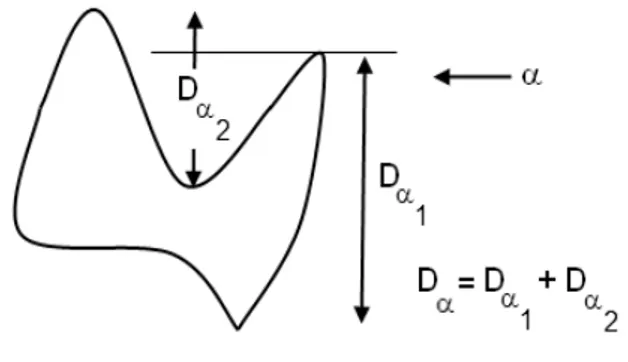
The diameter or diametral variation of a set is calculated in a given direction. It corresponds to half the cumulative length of all the projections in this direction of the boundaries of the set. We consider half this cumulative length because to any transition from the outside to the inside of the set, it corresponds necessarily an inside-outside transition and therefore two identical projections of boundary elements (Figure 3). We have Dα = Dα+π.

On a digital binary image, the diameters are computed for the main directions of the grid (three directions for the hexagonal grid and four for the square one). Each boundary element is determined by a Hit-or-Miss transform with a 01 double structuring element in the appropriate direction (operation actually performed with the diffNeighbor operator). The length l of each

projected boundary element (projection on a perpendicular line) is given by the following formulas, depending on the grid and the direction used (Figure 4):

Figure 3: Diametral variation Dα in direction

α

On the square grid, if i is the direction as it is coded in Mamba, the corresponding length li is given

by:

l₁=s_h

l₂=l₄=s_h×s_v/



l₃=s_v

Figure 4: Diameters projections on square and hexagonal grids

On the hexagonal grid, we have: l₁=l₃=2×s_h×s_v/



The diameter is finally given by:

Di = li . number_of_01_configurations_in_direction _i

5. Perimeter

The perimeter p of a set (which could be coarsely interpreted as the length of its boundary although, in the digital case, this analogy is really erroneous...) is given by applying a digital version of the Cauchy formula:

p= E



 D_=∫₀

D_d 

According to this formula, the perimeter is equal to π multiplied by the mean diameter of the set (averaged over all the directions). This formula is used directly in Mamba, the averaging being performed on three or four directions depending on the grid in use (hexagonal or square):

p=

k

∑

k

D_i

k is the number of directions used (3 with hexagonal grid, four with square grid).

6. Connectivity number

The connectivity number ν (also called Euler-Poincaré constant) is a non dimensional characteristic value of a set which is derived from the fundamental Euler formula for graphs (refer to [1]). For 2-dimensional sets, it can be obtained by the following formulas:

On an hexagonal grid:

=N0 0

1 −N 10 0

where N(.) represents the number of corresponding configurations in the image.

On a square grid (where the pixels belonging to the set are supposed to be 8-connected):

=N1 0

0 0−N 111 0N 1 001

For 2-dimensional sets, this connectivity number is equal to the difference between the number of connected components of the set and its number of holes. This connectivity number may be negative.

The connectivity number is calculated by simply counting the number of configurations used in the above formulas present in the image by means of Hit-or-Miss operators (with a particular care to avoid edge effects).

7. Number of connected components

This measure is simply provided by the image labelling algorithm (see Mamba documentation, [1]).

8. Feret diameters

The Feret diameters of a set (from René Féret, french engineer who studied the resistance of concrete during the 19th century) are the horizontal and vertical diameters of the rectangular bounding box of the set. They correspond to the horizontal and vertical pixel sizes of this box (provided by the extractFrame operator) multiplied respectively by the horizontal and vertical scale factors.

9. Results

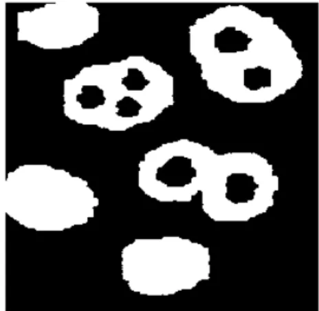
As an illustration, here are the results obtained by applying these various operators to the following binary image (Figure 5), in an hexagonal or square context (the scale factor is set to default):

Figure 5: Test image

Measure Hexagonal grid Square grid

Area 19989.0 19989.0 D1 784.0 726.0 D2 512.0 674.58 D3 772.0 512.0 D4 -- 657.61 Perimeter 2166.86 2018.62 Connectivity number -1 -1 Number of components 6 6

The index values in the diameters measures correspond to the directions in the grid in use. The diameter in direction 2 of the hexagonal grid is obviously equal to the diameter in direction 3 of the

square grid (it is the same direction and the scale factor is the same too).

We remark that the perimeter measurements are not identical for hexagonal and square grids. This is perfectly normal because the two sets which are measured are not identical (especially if we compare their respective boundaries). However, the two values are of the same order.

10. References

[1] Beucher, Nicolas (2010): Mamba Image Library Python Reference - http://mamba-image.org. [2] Serra, Jean (1982): Image Analysis and Mathematical Morphology - Academic Press..

(Publication date: January 21, 2011)

This document is copyrighted under the Creative Commons "Attribution Non-Commercial No