HAL Id: hal-01528537
https://hal.archives-ouvertes.fr/hal-01528537
Submitted on 31 May 2017
HAL is a multi-disciplinary open access
archive for the deposit and dissemination of
sci-entific research documents, whether they are
pub-lished or not. The documents may come from
teaching and research institutions in France or
abroad, or from public or private research centers.
L’archive ouverte pluridisciplinaire HAL, est
destinée au dépôt et à la diffusion de documents
scientifiques de niveau recherche, publiés ou non,
émanant des établissements d’enseignement et de
recherche français ou étrangers, des laboratoires
publics ou privés.
Bi-Layer textures: a Model for Synthesis and
Deformation of Composite Textures
Geoffrey Guingo, Basile Sauvage, Jean-Michel Dischler, Marie-Paule Cani
To cite this version:
Geoffrey Guingo, Basile Sauvage, Jean-Michel Dischler, Marie-Paule Cani. Bi-Layer textures: a Model
for Synthesis and Deformation of Composite Textures. Computer Graphics Forum, Wiley, 2017,
Proceedings of EGSR, 36 (4), pp.111-122. �10.1111/cgf.13229�. �hal-01528537�
Eurographics Symposium on Rendering 2017 P. Sander and M. Zwicker
(Guest Editors)
Volume 36(2017), Number 4
Bi-Layer textures:
a Model for Synthesis and Deformation of Composite Textures
Geoffrey Guingo1,2, Basile Sauvage2, Jean-Michel Dischler2and Marie-Paule Cani1
1Université Grenoble Alpes, CNRS (LJK), and Inria, Grenoble, France 2ICube, Université de Strasbourg, CNRS, France
+
*
*
+
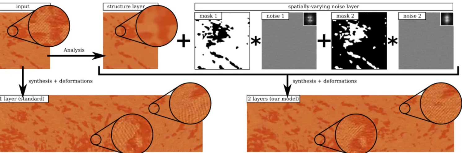
input Analysis synthesis + deformations structure layer1 layer (standard) 2 layers (our model)
synthesis + deformations
noise 1 noise 2
mask 1 mask 2
spatially-varying noise layer
Figure 1: Our noise model decomposes an input exemplar as a structure layer and a noise layer. The noise layer captures a spatially varying
Gaussian noise as a blend of stationary noises. Large outputs are synthesized on-the-fly by synchronized synthesis of the layers. Variety can be achieved at the synthesis stage by deforming the structure layer while preserving fine scale appearance, encoded in the noise layer.
Abstract
We propose a bi-layer representation for textures which is suitable for on-the-fly synthesis of unbounded textures from an input exemplar. The goal is to improve the variety of outputs while preserving plausible small-scale details. The insight is that many natural textures can be decomposed into a series of fine scale Gaussian patterns which have to be faithfully reproduced, and some non-homogeneous, larger scale structure which can be deformed to add variety. Our key contribution is a novel, bi-layer representation for such textures. It includes a model for spatially-varying Gaussian noise, together with a mechanism enabling synchronization with a structure layer. We propose an automatic method to instantiate our bi-layer model from an input exemplar. At the synthesis stage, the two layers are generated independently, synchronized and added, preserving the consistency of details even when the structure layer has been deformed to increase variety. We show on a variety of complex, real textures, that our method reduces repetition artifacts while preserving a coherent appearance.
CCS Concepts
•Computing methodologies → Texturing;
1. Introduction
Textures efficiently enhance objects with fine colored details and have therefore been ubiquitous for a long time in 3D virtual scenes. The recent improvements of graphics hardware and rendering tech-niques support the demand for increasingly detailed visual content.
In this context, by example texture synthesis, which allows the au-tomatic generation of textures from small size exemplars, has be-come a major challenge. It can either be used to support otherwise painstaking manual texture creation (enabling artists to focus man-ual edits where needed the most), or as an alternative to it.
c
2017 The Author(s)
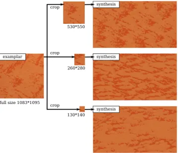
full size 1083*1095 crop 530*550 260*280 130*140 synthesis synthesis synthesis examplar crop crop
Figure 2: What you see is all you get: the smallest the input the
more repetitive the output, even using off-line optimization tech-niques [KNL∗15].
By example texture synthesis makes the fundamental assumption that the exemplar is representative of the underlying natural texture. Unfortunately, this assumption turns out to be wrong in many cases: exemplars are generally too small to cover the entire visual span of a given texture, leading to visual artifacts. As shown in Figure2, even the best optimization techniques cannot provide more variety than the exemplar. This strongly hampers realism. Moreover, op-timization leads to heavy computations and produces textures that are bounded.
Gaussian noise and tile-based methods are two alternative ap-proaches for generating unbounded textures on-the-fly (i.e. at run-time), from a single input exemplar. Whereas noise by example inherently avoids repetition artifacts, it can only handle homoge-neous textures and hardly manages non-Gaussian patterns, which represent the very large majority of textures. In reverse, tile-based methods, such as Wang tiles, are able to reproduce complex, non-Gaussian patterns with spatial variations, but since tiles are pre-generated using traditional synthesis approaches (like Graph-cut or optimization), they typically exhibit the previously mentioned strong repetition artifacts. The intuition is that spatial deformations can help to significantly reduce repetitions. However, if not done properly, fine scale patterns may be ruined, as shown in Figure1
bottom-left and Figure3top. Several works apply deformations in the synthesis process to create more varied contents, but the proper use of deformation has not been deeply tackled so far.
Our goal is to propose a more general, infinite on-the-fly tex-ture synthesis method, able to introduce variety when synthesizing natural textures. Many natural textures are composite, i.e. they ex-hibit different patterns at different locations (see dark and light pat-terns in Figure1). The variety lies in the structure (i.e. the shape, size and orientation of large patterns) while the consistency lies in the homogeneity of fine scale patterns. To achieve this, the insight
deformation (structure + noise)
deformation (structure) + noise
Figure 3: Pattern deformations produce variety provided that fine
grain appearance is preserved: rotation and stretching are shown on the usual 1-layer textures (top) versus our 2-layer model (bot-tom). Our model enables to deform structured patterns while pre-serving fine scale noisy patterns.
is to exploit the complementary nature of noise-based versus tile-based methods. The texture is decomposed into two additive layers: a structure layer captures spatial variations and non-Gaussian pat-terns, and is synthesized using tile-based approaches augmented by deformations (scaling, rotations and stochastic distortion fields); a noise layer captures fine scale Gaussian patterns and is synthesized with procedural methods. This solution implies solving two core is-sues: on the analysis side, quantifying noise and separating it from structure, as illustrated in Figure1top; and on the synthesis side, making the noise vary spatially according to the synthesized struc-ture. A major advantage of this bi-layered model is that deforma-tions of the structure produce variety while fine-scale consistency is maintained, as shown in Figure3bottom.
Our model is encoded using a combination of images (defin-ing the structure), power spectrum densities (defin(defin-ing noises), and masks (synchronizing noises over the structure). The main contri-butions are:
• A new model for spatially varying Gaussian noise: a few stationary noises are blended according to masks that encode non-stationarity (Section 3). To the best of our knowledge, this is the first method to analyze, describe and synthesize Gaussian noise with spatial variations. The key difficulty that we solve here is the spectrum estimation in the presence of spatial variations. We use clustering in the spectral domain and a new technique for computing power spectrum densities (PSD) through auto-correlation while some data is missing.
• A new bi-layered texture model: a noise layer captures fine scale Gaussian patterns, while a structure layer captures non-Gaussian patterns and structures (Section4). The key idea is to synchro-nize the layers through a set of masks enabling preservation of consistency. We can achieve unprecedented synthesis and deformation results compared to single layer models.
• An analysis method to instantiate our bi-layered model from a single input exemplar and very light user input (section5). The two layers, the masks and the spectra of the Gaussian patterns are then automatically computed.
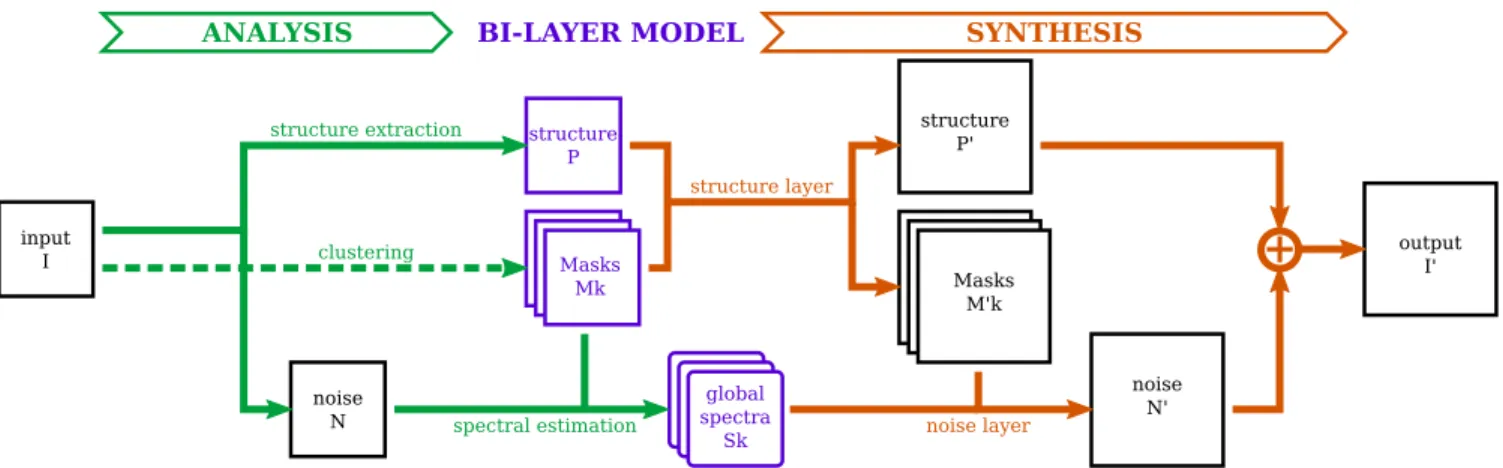
output I' structure P' input I structure P noise N Masks Mk structure extraction global spectra Sk noise N' structure layer noise layer Masks M'k
+
spectral estimation BI-LAYER MODEL ANALYSIS SYNTHESIS clusteringFigure 4: Processing pipeline. Our bi-layer model encodes textures using a structure layer (an image P), a set of Gaussian noises (spectra
Sk) and a set of localization masks (Mk). Analysis (left) consists in instantiating the model from a single input exemplar I: the structure is
extracted using filtering (I= P + N); the masks are computed using clustering; the spectra Skare computed using a new technique based on
auto-correlation. Synthesis (right) computes large composite outputs on-the-fly: a structure layer with masks is synthesized using a tile-based approach; a spatially-varying noise layer is synthesized procedurally from the spectra and the masks; the two layers are added to create the final texture.
For clarity reasons, these contributions are explained in separate sections3to5. They enable by-example texture synthesis, as sum-marized by the pipeline depicted in Figure4. An input exemplar I is analyzed (in green Figure4):
• A structure layer P is extracted by filtering I (Section5). • A noise layer is computed as N = I − P.
• Masks Mkare computed using clustering in the spectral domain (Section3.3). Each mask corresponds to one stationary noise. • Global spectra Sk(one per noise) are computed (Section3.3). Then, from the bi-layer model –encoded by P, Mkand Sk–, an out-put texture I′
= P′
+ N′is synthesized as the sum of two layers (in
orange Figure4):
• The structure layer P′ is synthesized using tile-based methods.
Masks M′
kare synthesized at the same time so as to encode syn-chronization with the noise (Section4).
• The spatially-varying noise layer N′blends stationary noises
(ac-cording to M′
k, see Section3.2) which are computed from their spectra Skby any state-of-the-art algorithm.
2. Related work
Most texture synthesis works address off-line synthe-sis [WLKT09], using for instance global optimization methods as initiated by [KEBK05]. But there is a recent need for "on-demand" generation of arbitrary sub-parts of a texture, as necessary for un-bounded on-the-fly texturing. Our work belongs to these on-the-fly texture synthesis methods. It is also related to texture synthesis with spatial deformation and to noise by example.
2.1. On-the-fly texture synthesis
By example on-the-fly texture synthesis methods can be classified into two approaches: 1) parallel, data-driven algorithms, 2) tiling techniques. On-the-fly data driven algorithms implement parallel
variants of pixel and patch-based synthesis algorithms, and suf-fer from the same limitations as their non-parallel counterparts. While parallel pixel-based approaches [LH05] require a feature map to preserve structure, parallel patch-based techniques [LL12] may produce visual repetition as well as possible seams. In both cases, the computational load is high, since these methods oper-ate on full neighborhoods, as opposed to individual surface points. These neighborhoods must be stored in a cache and are frequently accessed within iterative procedures, which reduces performance.
Tile-based techniques consist in creating puzzles, but (in con-trast with patch-based methods) use a pre-computed set of well-connecting texture tiles to generate an aperiodic tessellation of the plane. They are much faster than the previous parallel approaches and are thus better suited for real-time rendering applications. The pieces can either be generated from an exemplar, such as Wang and corner tiles [CSHD03,LD06] or computed procedurally [Sta97]. Patches with irregular shape have been used in [VSLD13], using an additional indirection to get rid of the explicit storage of large num-bers of pre-computed tiles. The core issue with these approaches is the fact that the same few pieces are repeated over and over again, since only the arrangements are random.
2.2. Texture synthesis with spatial deformation
By example synthesis methods never generate new texture features, so the result lacks visual variation if the supplied exemplar is too small or contains a salient and unique feature. A standard way of reducing feature repetition consists in applying noise-based spa-tial distortions (i.e. a random shift of texture coordinates), as done for near-regular textures in [LLH04] and for tile-based synthesis in [CJMW13]. This principle was introduced by Perlin [LLC∗10]
to add natural randomness to perfectly periodic structures. It was also experimented in [DG95], which argued that distortions should at least preserve some spectral characteristics of patterns such as
anisotropy. Some by example synthesis techniques have used de-formation like the feature matching and dede-formation synthesis ap-proach of [WY04] and the graph-cut texture synthesis [KSE∗03].
In the latter case, deformation is used to give a perspective dis-tortion impression. In all cases, the principle is simple: the defor-mation is applied to the input and added to the pool of potential patches / neighbors to select contents. But all techniques have a strong drawback: spatial distortions may corrupt the visual char-acteristics of "sub-patterns", as for instance a cement pattern on a brick that would be stretched at the same time as the brick.
Our approach builds on tile-based methods. By separating noise patterns from structure, it improves the visual variety and extends the range of acceptable deformations: the structure can be distorted, stretched or rotated while the underlying noise patterns are pre-served (see Figure3).
2.3. Composite texture models
A composite texture model represents a texture as an assembly of simpler sub-textures. It is often defined as a two-layered model, where one layer is a label map indicating where the different sub-textures are located [ZFCVG05]. The label map defines a parti-tion of the plane. Some methods first synthesize a label map, and then fill the result with different sub-textures [RCOL09]. There are however two difficult issues: segmenting an input image into sub-textures and synthesizing sub-textures by taking into account transitions between them. Optimization and off-line synthesis tech-niques can partly resolve the latter issue [WWY14].
At first glance, our approach resembles composite texture syn-thesis. However, it differs on a fundamental aspect: we do not use any label map, but only use additive layers. What we call "struc-ture" in our model is a filtered color pattern image, as opposed to a label map. The filtered image is linearly combined with a weighted sum of stationary noises. This comes up with several advantages. Firstly, extracting "noise" is easier than texture seg-mentation, because a spectral metric can be used instead of texture classification algorithms [LSA∗16]. Secondly, our structure can be
synthesized with any existing on-the-fly tile-based synthesis tech-nique [CSHD03,LD06,VSLD13], provided that we integrate into the procedure the weights of the different noises. Lastly, station-ary noise can be easily synthesized on-the-fly using pseudo-random number generation.
2.4. Noise by example
Noise by example [GLLD12,GDG12] allows the generation of a parametric noise function from an example image. Such noises cor-respond to sub-classes of irregular textures, called Gaussian tex-tures. Procedural noise inherently allows for infinite texturing with-out repetition. However, Gaussian textures are rare (actually, none of the textures found for instance in the textures.com database is Gaussian). The lack of structure can be addressed by fixing some phases in the power spectrum [GSV∗14]. This approach is however
biased since structure might be spread all over the spectrum, so a binary separation of frequencies is most often not adequate.
An efficient noise synthesis technique inspired by Spot-noise [vW91] has recently been proposed in [GLM17], based on
sparse convolution with a so-called “texton”. The authors propose to mix noises by interpolating between textons, which allows for smooth spatial variations. However, no exemplar analysis is pro-vided to separate different noises, and the method is restricted to Gaussian textures.
The random phase component is assumed stationary with all of these techniques. However, noise characteristics are not stationary for most natural textures. A similar problem appeared in [JCW11], where diffusion curves are textured using Gabor noise with spa-tially varying parameters, so as to get a vector representation of bitmap images. Gabor filter banks are applied on disks of 40 pixels diameter around the pixels to evaluate local main frequency com-ponents. But as mentioned by the authors, “this allows recording a single dominant frequency that captures only a rough impression of many textures”. This is sufficient for image vectorization but not for texture synthesis. We show that large spectra are necessary to capture good quality noise patterns. One of our major contributions is to be able to evaluate such spectra using a novel approach based on auto-correlation.
The next section describes our new noise model. Its combination with a structure layer will be discussed in Section4.
= +
N
*
M1 N1
*
M2 N2
Figure 5: Spatially varying Gaussian noise. Each SV-noise (N)
is a blend of stationary noises (Nk) defined by spectra (inset) and
weighed by masks (Mk).
3. Spatially varying Gaussian noise 3.1. Stationary noise
A Gaussian noise is characterized by its power spectrum distribu-tion (PSD), which represents how the power S2is distributed across frequencies f , where S is the magnitude of noise’s spectrum (we will call S "spectrum" in the derivations below for readability).
Phase randomization, that we call Random-Phase Noise (RPN), is a technique to estimate a random realization of a stationary Gaus-sian noise from a given PSD:
RPN(x) =
∑
fS( f ) cos( f x + ϕ( f )) (1) where the phases ϕ( f ) are randomly picked. State-of-the-art mod-els and algorithms are able to analyze a discrete input by comput-ing its PSD and to synthesize on-the-fly a continuous non-repetitive
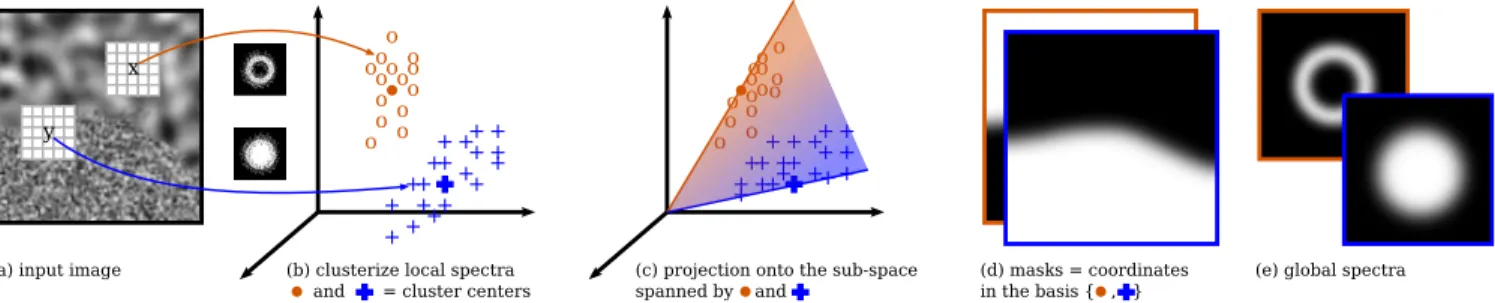
(b) clusterize local spectra and = cluster centers
+ ++ + + + ++ + + + + + + + + + + + + o o o o o o o o o o o oo o
(a) input image x y
(c) projection onto the sub-space spanned by and + ++ + + + ++ + + + + + + ++ + + + + o o o o o o o o o o o oo o + + (d) masks = coordinates in the basis { , }+
(e) global spectra
Figure 6: Noise by example: computation of masks and basis. Local spectra Slocx are computed by Welch’s method on small windows around
pixels x of the input (a). A clustering (b) provides cluster centers Slock which span a subspace onto which the local spectra are projected (c). The coordinates are forced to be positive to get the masks (d). The global spectra Skare computed by our new estimator based on
auto-correlation (e).
infinite output [GLLD12,GSV∗14]. They rely on variants of
Equa-tion (1) so they assume stationarity, i.e. the spectrum S is assumed to be independent from the position x.
3.2. Spatial variations
To make the noise vary spatially, we would like the spectrum S to depend on the position x. We achieve this by defining a spatially-varying(SV)-noise N as: N(x) = K
∑
k=1 Mk(x)Nk(x), (2) where Mkare scalar blending masks, and Nkare stationary noises described by “global” spectra Sk(see Figure5). An advantage of this solution is to separate spatial variations – encoded in Mk(x) – and spectral information – encoded Sk( f ).The intuition is that, thanks to linearity of Equation (1),
N is then characterized around x by the “local” spectrum Sx( f ) = ∑kMk(x)Sk( f ), provided that the phases φ are the same for all k, that is the noise realizations are not independent. Enforc-ing φ this way solves for the optimal transport on the Gaussian dis-tributions, which has been proven to be appropriate to interpolate Gaussian noises [XFPA14].
Based on state-of-the-art methods for stationary noises, SV-noise can be synthesized efficiently: each Nkis synthesized using a ran-dom phase approach (e.g. Equation (1) with S = Sk) or a sparse convolution [GLM17]; then they are blended with weights Mk. On-the-fly synthesis also requires the masks to be synthesized on-the-fly. This can be done using any state-of-the-art method, e.g. noise or tiles. We refer to Section4since synthesizing an SV-noise is a particular case of our two-layers model, where the structure layer is empty. Figure5shows a synthetic example of spatially-varying noise (SV-noise).
3.3. Noise by example
Let us now address the problem of instantiating the noise model of Equation (2) from an input exemplar: given a spatially varying noise exemplar I, we derive a set of masks {Mk} and spectra {Sk} in the following way. We view our model as a decomposition of
(a) Input (b) Tloc= 4 (c) Tloc= 8 (d) Tloc= 32
Figure 7: Computation of masks Mkfrom an SV-noise input (a).
Top row: normalized distanceskSloc
x − Slock k. Bottom row: binary
masks. The larger Tloc the better the discrimination but the less precise the boundaries. A good strategy is to set Tloc as small as possible to get precise masks while still discriminating regions.
the noise in a basis {Sk}, where the masks {Mk} used as weighing factors play the role of spatially-varying coordinates with respect to these noises. The difficulty is that neither the basis nor the coordi-nates are known. We solve the problem using the process illustrated in Figure6, described next.
Mask estimation. First, we estimate the local spectra Slocx of size Tloc using Welch’s method [Wel67] in a small window cen-tered at each pixel x. They describe the local frequency content around x. Then, we run a clustering algorithm on {Sloc
x } to get K representative cluster centers Sloc
k , 1 ≤ k ≤ K. We use a K-means algorithm with a number K of seeds provided by the user. Then, for each pixel, Sloc
x is projected onto the subspace spanned by the ba-sis {Sloc
k }. The coordinates in this basis are the mask values Mk(x), provided that they are positive.
We experimented several alternatives for projecting Sloc x . Or-thogonal projection is not appropriate because it provides many large or negative coordinates. So, we computed a convex barycen-ter of {Sloc
k } that preserves the relative distances kSlocx − Slock k. This is robust but boundaries are blurred, as shown in Figure 7: the larger Tloc the more robust, but the more blur. So Tloc must be c2017 The Author(s)
T = 64 T = 32 T = 16 T = 8 T = 8 T = 16 T = 32 T = 64 inp ut s s y nt he s iz e d noi s e s
Figure 8: Noise synthesis. The larger the spectrum size T the better
the reproduction. In all our examples we used T= 64.
large enough to capture the noise spectrum, although many natu-ral textures exhibit sharp boundaries. Hence, when transitions are sharp we used binary masks. Mk(x) = 1 iff Sxlocbelongs to cluster k.
We could expect Sloc
k to be good estimates for Sk. However, es-timating local spectra requires to use windows smaller than spa-tial variations, typically 4 ≤ Tloc≤ 16 for our examples, as il-lustrated in Figure7. Conversely, spectra for synthesis must have much higher resolution, typically T ≥ 64, as illustrated in Figure8. Common spectrum estimation techniques require large windows of stationary signal. However, they cannot be applied in our case be-cause of the spatial variations. So, we developed a new technique based on auto-correlation.
Spectral estimation with missing data. The PSD of a signal is equal to the Fourier transform of its auto-correlation AC. If I is a stationary signal with finite power, AC can be estimated over a
T× T window Y by
ACY(x) = 1
|Y |y∈Y
∑
I(y)I(y + x) (3)where positions y + x are computed modulo T . In our case I is not stationary over large windows, but approximately piecewise sta-tionary over regions within Y . We propose to estimate AC over the pairs of pixels lying both inside the region of interest:
ACYM(x) = 1
|M ∩Y |yand x+y∈M∩Y
∑
I(y)I(y + x) (4) where M is a binary mask of the region. The FFT of ACMY provides a noisy estimate of the spectral content within the region. To reduce noise while maintaining the resolution, we make use of averaging. That is, we pave I with square windows Y and estimate the PSD as an average over the different windows, weighted by the number of pixels:
S2= 1
∑ |M ∩Y |
∑
Y |M ∩Y | dAC MY ( f ) (5) The estimator (5) is amazingly robust to regions with complex shapes and sparsity |M ∩ Y |/|Y | ≥ 70%. We use it to estimate each Sk with M covering 90% of the cluster k (the 90% closest to Sloc
k ). In practice we used T = 64 in all our examples.
Parameter tuning. We are left with two parameters. The first one is the number K of clusters, which is easy to provide: it equals the number of different random patterns perceptually salient to the user in the input exemplar, generally 2 to 4. The second parameter is the size Tlocof the local spectra. We refer the reader to Section4for a user-friendly technique to set it, based on visual evaluations. 4. Bi-layer textures
For clarity reasons, we present our model for greyscale textures and refer to section6for the management of colors. Our texture model is inspired by real textures, which often exhibit strongly structured patterns locally enhanced with noisy patterns. As shown in Figure1
top, we decompose a texture I as a sum
I(x) = P(x) + N(x) = P(x) + K
∑
k=1
Mk(x)Nk(x), (6) where P is a structure layer and N is a spatially varying noise layer defined as in Section3. Thus a texture is encoded by:
• P: an image representing the structure layer, • Sk: scalar maps representing the spectra of noises Nk, • Mk: scalar maps representing the masks of noises Nk.
The motivation is to take benefits from the different synthesis techniques that can be used for the two layers (see Figure4). To cre-ate a new texture image, a new structure layer P′together with new
masks M′
kare first synthesized from P and {Mk}. State-of-the-art tile-based methods can be used at this stage because they are appro-priate for highly structured textures. The masks are treated as extra channels that correlate with P: they undergo the same operations (cut, copy, paste, blend, deform) as P. In a second stage, an SV-noise layer is synthesized using the procedural methods described in Section3. The key idea here is that the masks serve as synchro-nization maps between structure and noise, by selecting which ran-dom pattern in N is added to which structured pattern in P. Indeed, since the masks are synthesized simultaneously with the structure, they can be used to guide the spatial variations of the noise.
Input
Input
Wang tiling Our method
Input
Content exchange
Figure 9: Synthesis results using Wang tiling [CSHD03], con-tent exchange [VSLD13], and content exchange plus rotations and stretching using our bi-layer model.
Let us now discuss the benefits of this bi-layered model over standard, single-layered textures. To synthesize the structure we could used off-line techniques, for example based on graph-cut [KSE∗03]. However, we aim at on-the-fly-synthesis. Remember
we want to apply deformations. We chose to apply deformations on-the-fly, so as to maximize the variety without extra memory cost. To do so, we modified the mono-scale version of [VSLD13], i.e. without complex color transfers and texture fetches. It consists in Wang tiles, in which patch contents are randomly exchanged. We modified the algorithm by allowing for contents to be rotated (by angle θ ∈ {π/4, π/2, 3π/4, π}) and scaled (0.5 ≤ λ ≤ 1).
In Figure9, we compare the results of our technique with related synthesis techniques. Wang tiling exhibits repetitions and align-ment artifacts, here, due to a low number of borders (2 times 2 resulting in 16 tiles) and to salient perceptual features on some of the tile borders. The tiles were generated with a patch-based al-gorithm. Content exchange reduces alignments, but repetitions are still visible. The addition of spatial deformations, made possible by our bi-layer model, reduces repetition artifacts (Figure9last col-umn). If applied to a single layer (Figure10), the fine-scale Gaus-sian patterns are deformed, strongly altering the appearance. Note also, that our model contributes to hide seams introduced along patch boundaries, in two ways: deformations ease feature align-ment along boundaries; the noise layer covers seams and make them less visible.
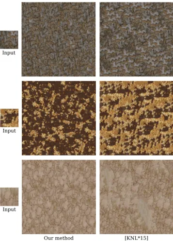
In Figure11, we compare our on-the-fly technique with one of the best current off-line synthesis technique [KNL∗15]. It shows a
slight quality loss, which is due to seams in the structure and ap-proximation of the noise spectra. In return, we provide much more
Input
Input
Single layer Our bi-layer model Input
Figure 10: Comparison single layer versus bi-layer. Structure is
deformed using scaling, rotations and turbulence. See how the fine patterns are distorted with single layer.
variety, speed (on-the-fly versus tens of minutes) and scalability (unbounded textures).
In Figure 12, we compare with noise by example and LRP-noise [GSV∗14] which also separates structure and noise. Our
method has several advantages. First, LRP-noise assumes that the noise is stationary while we manage spatial variations, which dra-matically increases the set of textures it applies to. Second, our structure has much better quality (see section5for details). Third, the structure in [GSV∗14] is periodic up to small distortions:
rota-tions or stretching are not possible. Eventually intricate shader im-plementation is required to reduce the computation overhead due to fixed phases in the structure, while we can rely on any tiling technique.
5. Analysis of input exemplars
In this section, we tackle the problem of instantiating our model from an input exemplar, i.e. computing P, {Mk}, and {Sk} from an input image I. We consider greyscale textures and refer to section6
for the management of colors.
In Section3.3we described a solution to this problem for purely Gaussian, spatially varying noise, i.e. with no structure layer P. We build on this simpler case to solve the full problem (see Figure4): • The structure layer P is extracted from I (see details below). • The noise layer is computed as N = I − P.
• The masks Mkare computed as in Section3.3. Note that the local c2017 The Author(s)
elfTuning 9 [KNL*15] Input Input Input Our method
Figure 11: Comparison with off-line optimization [KNL∗15]. Op-timization reproduces cleaner and sharper features. Our method provides more variety and on-the-fly synthesis.
spectra Sloc
x are estimated on I, which contains not only noise. We could have used N instead, however we would have had to do without useful information contained in I, such as the average intensity (or color).
• The global spectra Skare computed as in Section3.3. Note that the local spectra are computed on N (not I) because they must encode the noise layer only.
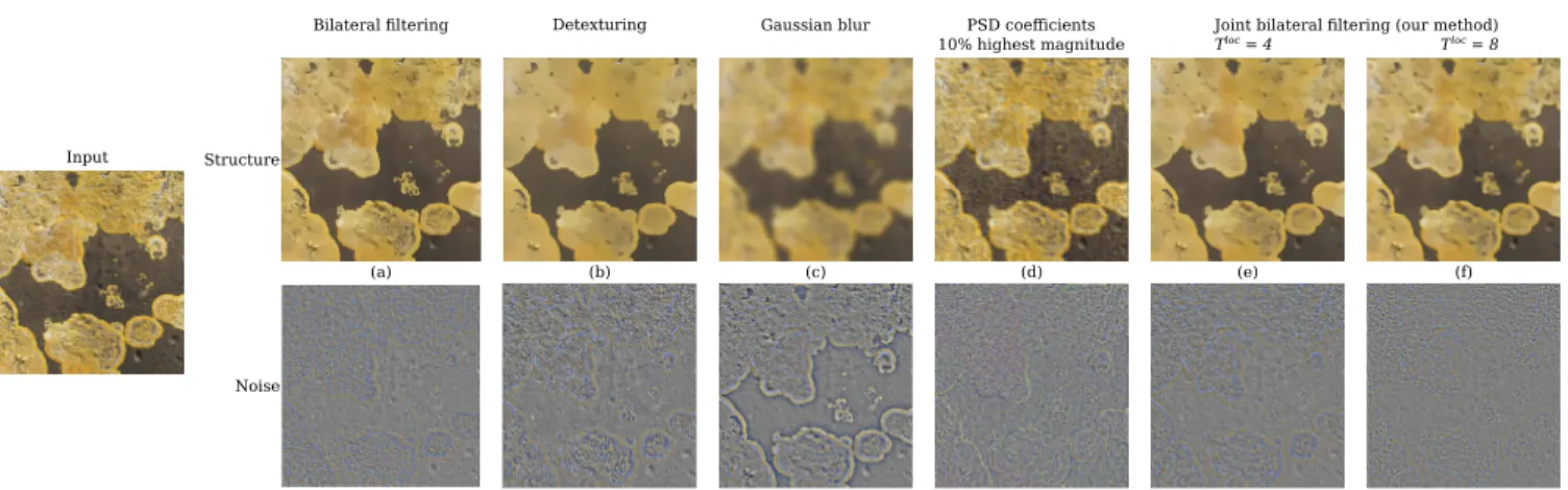
The computation of P from I is somewhat similar to de-texturing and to de-noising, but with important differences preventing us from using some previous solution. We show a comparison in Fig-ure13and other ones are provided in the supplemental material. De-texturing [XYXJ12,CLKL14] aims at removing small scale patterns (e.g. tile pieces in a mosaic) while preserving large ones (e.g. the global image of the mosaic). In our case, a criterion for scale is not relevant: in the mosaic example, we would like the piece borders to be kept in P, because they are highly structured. De-noising aims at removing a random additive error from an image, and so do we. Gaussian smoothing adds too much blur. Bilateral filtering performs well, if each region has its own color. However, we want each region to have its own spectrum. Our solution there-fore consists in joint bilateral filtering [PKTD09] guided by the
lo-(a) Input
(b) RP-noise
(c) LRP-noise Structure
(d) Our method Structure
Figure 12: Comparison to noise by example. The example (a)
con-tains two regions with different noises. Random phase noise (b) can not reproduce the underlying structure. Local random phase noise (c) extracts a blurred structure and can not manage spatial variations in the noise. Our technique (d) extracts a sharper struc-ture and well reproduces spatial variations.
cal spectra Sloc
x . This way, two pixels x and y are averaged, if they have similar local spectral characteristics. That is, if kSloc
x − Sylock is
small. Our method has proven to be versatile, though de-texturing and bi-lateral filtering also perform well on some examples.
We compared our structure extraction method with [GSV∗14],
which defines the structure in the spectral domain as the frequen-cies having the largest magnitude. As noticed by the authors, it mostly selects low frequencies, while high frequencies often con-tribute to sharp features that we want to be preserved in the struc-ture. Figures12and13show that our method based on spatial fil-tering compares favorably.
Bilateral filtering Detexturing Gaussian blur PSD coefficients 10% highest magnitude
Joint bilateral filtering (our method)
Tloc = 4 Tloc = 8
Structure
Noise Input
(a) (b) (c) (d) (e) (f)
Figure 13: Structure extraction. Bilateral filtering and de-texturing perform well in some cases. Gaussian smoothing blurs sharp edges.
Thresholding the PSD fails when high frequencies contribute to the structure. Our joint bilateral filtering driven by local spectra is versatile.
To make the method user-friendly, we only keep a single param-eter under the user control. In all our examples, we fixed the joint bilateral filter parameters as follows: spatial neighborhoods are 16 pixels wide; the standard deviation for the distance between spectra is set to 0.01; the filter is iterated 5 times. The only parameter left is the size Tlocof the local spectra. The larger Tloc, the more in-formation is filtered into N, and possibly the more blurry P will be, leading to possible artifacts in the synthesis. The smaller Tloc, the more information is preserved in P, the more faithful the synthesis, but the less deformations can be introduced. We argue that the good value for Tlocis the one that produces the best synthesis, which is, in the end, a visual criterion. Thus, we ask the user to select the best size for Tlocamong a small set of values (Tloc= 2, 4, 8, 16), based on the visual quality of synthesized examples, see figure14. The user is shown, for each Tloc, the layers P and N, as well as a result with N synthesized over the same P. The best choice is the largest possible Tlocleading to acceptable visual results. Many examples are shown in the supplemental material to this paper.
Input T loc=2 T loc=4 T loc=8 T loc=16
Figure 14: Tuning of the analysis. The user is shown a set of
syn-thesis examples (top) along with the layers P (middle) and N (bot-tom). He selects the largest value Tlocas long as the visual quality is acceptable. Here Tloc= 4 or 8 would probably be appropriate.
6. Extensions
Colored textures. Colors require modifications in our pipeline. The analysis of a colored input is driven by the luminance chan-nel: local spectra are computed on the luminance, then the com-putation of masks and the structure extraction are unchanged. This leads to colored layers P and N. The synthesis of structure from P requires no modification. The critical stage is the synthesis of noise because wrong correlations of the RGB channels may create new colors. We treat each noise Nkseparately, because they tend to have much less color variations than the global image. Random phase shift [GGM11] can not be used because our PSD estimation pro-vides no phase. So each noise is computed in its own color space with channels as independent as possible, resulting from a per-cluster PCA in the RGB space. The channels are then synthesized independently.
Anti-aliasing. Texture anti-aliasing is an issue when rendering 3D scenes. In particular flickering artifacts are caused by undersam-pling of large scenes. Our model is compliant with the available techniques for each layer. Regular tilings, which are suitable for the structure layer, generally support MIP-mapping. Note however that no precise pre-filtering is known for content exchange [VSLD13]. The noise layer can be filtered directly in the spectral domain by fading out high frequencies.
Histogram equalization for non-Gaussian noises. Our model a priori requires the noise layer N to be Gaussian, which is not guar-anteed. One can loosen this constraint by adding a histogram equal-ization, that operates on the noise layer only, cluster, and per-channel. This widens the set of textures that can be faithfully repro-duced, as shown in Figure15. Moreover, this method is compliant with anti-aliasing [HNPN14].
Improving sharp pattern borders. As discussed in Section5, choosing the size of local spectra is a compromise: good discrim-ination of the patterns may require large windows and imply blur-ring of both the masks and the structure borders. In all our results we used binary masks to sharpen the noise transitions (see Sec-tion3.3). However this does not remove blur in the structure.
Input Structure Noise Synthesis with equalization Synthesis without equalization
Figure 15: Histogram equalization is applied to the noise layer. It
improves synthesis results when the noise is not Gaussian.
ure16shows how we can sharpen structure borders by modifying the P + N decomposition. In a small band along the region border
Nis forced to vanish so sharp borders are preserved in P.
7. Results and discussion
Results. The results of our method are presented through Figures9
to16and in the series of high-resolution images attached as sup-plementary documents. We showed in Section3that we improve over noise-based approaches by controlling spatial variations. We showed in Sections4and5that our bi-layered model compares fa-vorably to both purely tile-based and LRP-noise approaches. Our method however comes with a number of limitations.
Limitations. Firstly, our method cannot work if fine scale patterns in the input exemplars are not Gaussian. In Figure17, we show an example where what remains after structure extraction is a struc-tured sub-texture, which cannot be reproduced using a noise model. We could overcome this problem by using our approach in a recur-sive way, i.e. recurrecur-sively extracting structure layers until only noise remains. Secondly, several steps of our processing pipeline could be improved. The computation of masks sometimes lack sharpness, and our projection method prevents control of intensity variations because the masks sum up to 1. Also the structure extraction some-times still blurs borders of some structured patterns (see Figure16
top).
Performance of the synthesis. The synthesis time is exactly the sum of times for both layers, thus it depends on the algorithms cho-sen. We implemented the noise layer by large pre-computed peri-odic tiles: repetition is not visible because of the structure layer. An alternative is to use texton noise [GLM17]. In this context, the bottleneck is the number of texture/memory accesses : 1 for Wang tiles, 2 for patch exchange, 3 + K for our technique (when there are less than 4 noises, all masks fit in a single texture). As a compari-son, [LH05] requires more than 100 accesses for their full padded pyramid.
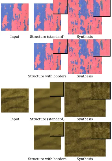
Structure with borders Synthesis
Synthesis Structure with borders
Structure (standard) Synthesis Input
Synthesis Structure (standard)
Input
Figure 16: Top row: sharp borders of the input (left) may be
smoothed in the structure (middle) and degraded during synthe-sis (right). Second row: the quality may be improved by exactly preserving a thick border (right) in the structure. In some cases however alignments may be broken (see the fabric).
Performance of the analysis. Many parameters have impact on the off-line analysis, so we provide ranges for 512 × 512 input ex-emplars. The main stages of computation are:
• The structure extraction needs a pre-computation of local spectra (1 to 6 min depending on Tloc) and the filtering (1 min). • Computing the masks mainly relies on a K-means clustering,
which converges very quickly (less than 20 iterations).
• Estimating the global spectra is the most time consuming, up to 1 hour for 3 channels. It relies on the auto-covariance computa-tion (equacomputa-tion (5)), which depends on the size T , on the sparsity threshold, and on the shape of the masks. Note that this stage is implemented on CPU and could be parallelized.
8. Conclusions
In this paper we presented a new model for spatially varying Gaus-sian noise, expressed as spatial blending of stationary noises. It
Input Structure Noise
Synthesis
Figure 17: Limitation. The fibers within the noise layer are not
Gaussian patterns. Our method fails to synthesize them.
comes with an algorithm for analyzing an input exemplar. Of par-ticular interest is a new spectral estimation technique for noises de-fined over a region with arbitrary shape (missing data). This model is part of a bi-layered model for representing textures as a sum of a structure layer and a noise layer, synchronized through a set of masks.
Our model supports on-the-fly synthesis, based on random-phase or sparse convolution techniques for the noise layer and tiling for the structure layer. We take advantage of both approaches: tiling well reproduces structured patterns, while noise reduces artifacts. The main advantage of our model is to enable spatial deformations of large structured patterns, while fine Gaussian patterns are pre-served. It greatly improves the variety of the synthesized textures.
We provide analysis from an input exemplar. A structure extrac-tion technique is based on joint bilateral filtering. To make this anal-ysis pipeline user-friendly, we carefully reduce user-tuning to two parameters: the number of random patterns (usually 2 to 4); the size of local spectra, for which we provide a visual choice among a few pre-selected values.
Note that while we selected or designed a consistent set of pro-cessing methods throughout the pipeline, several of them could be modified or replaced without changing the other stages. In particu-lar, we believe there is room for improvements in the computation of masks and in the extraction of structure, which are closely re-lated to image processing tools.
Another promising perspective is to decide the appropriate de-formations from the input itself. While stretching and rotations are easy to tune manually, more complex deformations – such as dis-tortions, bending or shearing – remain challenging.
Besides, some applications are worth being investigated as future extensions of our approach: they include texture transfer, which usually faces distortion problems that could be solved using our bi-layered approach; and texture extraction from images and videos, because it requires pattern description and comparison.
Acknowledgements
This work has been partially funded by the project HDWorlds from the Agence Nationale de la Recherche (ANR-16-CE33-0001) and by the advanced grant 291184 EXPRESSIVE from the Euro-pean Research Council (ERC-2011-ADG 20110209). We would like to thank Sylvain Thery for the help provided in the develop-ment, and Sarah Kushner for english proof-reading. Image Cour-tesy: www.mayang.com/textures/
References
[CJMW13] CHEN K., JOHAN H., MUELLER-WITTIG W.: Simple and efficient example-based texture synthesis using tiling and defor-mation. In Proceedings of the ACM SIGGRAPH Symposium on In-teractive 3D Graphics and Games(New York, NY, USA, 2013), I3D ’13, ACM, pp. 145–152. URL:http://doi.acm.org/10.1145/ 2448196.2448219,doi:10.1145/2448196.2448219.3
[CLKL14] CHO H., LEE H., KANG H., LEE S.: Bilateral tex-ture filtering. ACM Trans. Graph. 33, 4 (July 2014), 128:1– 128:8. URL: http://cg.postech.ac.kr/research/btf/, doi:10.1145/2601097.2601188.8
[CSHD03] COHENM. F., SHADEJ., HILLERS., DEUSSENO.: Wang tiles for image and texture generation. ACM Trans. Graph. 22, 3 (July 2003), 287–294. URL: http://doi.acm.org/10.1145/ 882262.882265,doi:10.1145/882262.882265.3,4,7
[DG95] DISCHLER J., GHAZANFARPOUR D.: A geometrical based method for highly complex structured textures generation. Comput. Graph. Forum 14, 4 (1995), 203–216. URL:http://dx.doi.org/ 10.1111/1467-8659.1440203,doi:10.1111/1467-8659. 1440203.3
[GDG12] GILETG., DISCHLERJ.-M., GHAZANFARPOURD.: Multiple kernels noise for improved procedural texturing. Vis. Comput. 28, 6-8 (June 2012), 679–66-89. URL:http://dx.doi.org/10.1007/ s00371-012-0711-2,doi:10.1007/s00371-012-0711-2. 4
[GGM11] GALERNEB., GOUSSEAUY., MORELJ.-M.: Random phase textures: Theory and synthesis. IEEE Transactions on Image Processing 20, 1 (2011), 257 – 267.9
[GLLD12] GALERNEB., LAGAEA., LEFEBVRES., DRETTAKISG.: Gabor noise by example. ACM Trans. Graph. 31, 4 (July 2012), 73:1–73:9. URL:http://doi.acm.org/10.1145/2185520. 2185569,doi:10.1145/2185520.2185569.4,5
[GLM17] GALERNEB., LECLAIRE A., MOISAN L.: Texton noise. Computer Graphics Forum (2017), n/a–n/a. doi:10.1111/cgf. 13073.4,5,10
[GSV∗14] GILET G., SAUVAGE B., VANHOEY K., DISCHLER J.-M., GHAZANFARPOUR D.: Local random-phase noise for proce-dural texturing. Transactions on Graphics 33, 6 (November 2014), 195:1–195:11. (Proceedings of Siggraph Asia’14). doi:10.1145/ 2661229.2661249.4,5,7,8
[HNPN14] HEITZE., NOWROUZEZAHRAID., POULINP., NEYRETF.: Filtering Non-Linear Transfer Functions on Surfaces. IEEE Transac-tions on Visualization and Computer Graphics 20, 7 (July 2014), 996– 1008. URL: https://hal.inria.fr/hal-00876432, doi: 10.1109/TVCG.2013.102.9
[JCW11] JESCHKES., CLINED., WONKAP.: Estimating color and tex-ture parameters for vector graphics. Computer Graphics Forum 30, 2 (Apr. 2011), 523–532. URL:https://www.cg.tuwien.ac.at/ research/publications/2011/jeschke-2011-est/.4
[KEBK05] KWATRAV., ESSAI., BOBICKA., KWATRA N.: Texture optimization for example-based synthesis. ACM Trans. Graph. 24, 3 (July 2005), 795–802. URL: http://doi.acm.org/10.1145/ 1073204.1073263,doi:10.1145/1073204.1073263.3
[KNL∗15] KASPAR A., NEUBERT B., LISCHINSKI D., PAULY M., KOPFJ.: Self tuning texture optimization. Comput. Graph. Forum 34, 2 (2015), 349–359. URL:http://dx.doi.org/10.1111/cgf. 12565,doi:10.1111/cgf.12565.2,7,8
[KSE∗03] KWATRA V., SCHÖDL A., ESSA I., TURK G., BO -BICK A.: Graphcut textures: Image and video synthesis using graph cuts. In ACM SIGGRAPH 2003 Papers (New York, NY, USA, 2003), SIGGRAPH ’03, ACM Siggraph, ACM, pp. 277–286. URL: http://doi.acm.org/10.1145/1201775.882264, doi:10.1145/1201775.882264.4,7
[LD06] LAGAEA., DUTRÉP.: An alternative for wang tiles: Colored edges versus colored corners. ACM Trans. Graph. 25, 4 (Oct. 2006), 1442–1459. URL:http://doi.acm.org/10.1145/1183287. 1183296,doi:10.1145/1183287.1183296.3,4
[LH05] LEFEBVRES., HOPPEH.: Parallel controllable texture synthe-sis. ACM Trans. Graph. 24, 3 (July 2005), 777–786. URL:http:// doi.acm.org/10.1145/1073204.1073261,doi:10.1145/ 1073204.1073261.3,10
[LL12] LASRAMA., LEFEBVRES.: Parallel patch-based texture syn-thesis. In Proceedings of the Fourth ACM SIGGRAPH / Eurograph-ics Conference on High-Performance GraphEurograph-ics(Aire-la-Ville, Switzer-land, SwitzerSwitzer-land, 2012), EGGH-HPG’12, Eurographics Association, pp. 115–124. URL: http://dx.doi.org/10.2312/EGGH/ HPG12/115-124,doi:10.2312/EGGH/HPG12/115-124.3
[LLC∗10] LAGAEA., LEFEBVRE S., COOK R., DEROSE T., DRET -TAKISG., EBERTD., LEWISJ., PERLINK., ZWICKERM.: A sur-vey of procedural noise functions. Computer Graphics Forum 29, 8 (2010), 2579–2600. URL: http://dx.doi.org/10.1111/j. 1467-8659.2010.01827.x, doi:10.1111/j.1467-8659. 2010.01827.x.3
[LLH04] LIUY., LINW.-C., HAYSJ.: Near-regular texture analysis and manipulation. In ACM SIGGRAPH 2004 Papers (New York, NY, USA, 2004), SIGGRAPH ’04, ACM, pp. 368–376. URL:http:// doi.acm.org/10.1145/1186562.1015731,doi:10.1145/ 1186562.1015731.3
[LSA∗16] LOCKERMAN Y. D., SAUVAGE B., ALLÈGRE R., DIS -CHLER J.-M., DORSEYJ., RUSHMEIER H.: Multi-scale label-map extraction for texture synthesis. ACM Trans. Graph. 35, 4 (July 2016), 140:1–140:12. URL:http://doi.acm.org/10.1145/ 2897824.2925964,doi:10.1145/2897824.2925964.4
[PKTD09] PARIS S., KORNPROBST P., TUMBLIN J., DURAND F.: Bilateral filtering: Theory and applications. Foundations and Trends in Computer Graphics and Vision 4, 1 (2009), 1–73.R URL:http://dx.doi.org/10.1561/0600000020,doi:10. 1561/0600000020.8
[RCOL09] ROSENBERGERA., COHEN-ORD., LISCHINSKID.: Lay-ered shape synthesis: Automatic generation of control maps for non-stationary textures. In ACM SIGGRAPH Asia 2009 Papers (New York, NY, USA, 2009), SIGGRAPH Asia ’09, ACM, pp. 107:1– 107:9. URL: http://doi.acm.org/10.1145/1661412. 1618453,doi:10.1145/1661412.1618453.4
[Sta97] STAMJ.: Aperiodic texture mapping. Tech. Rep. ERCIM-01/97-R046, European Research Consortium for Informatics and Mathematics (ECRIM), 1997.3
[VSLD13] VANHOEYK., SAUVAGEB., LARUEF., DISCHLERJ.-M.: On-the-fly multi-scale infinite texturing from example. ACM Trans. Graph. 32, 6 (Nov. 2013), 208:1–208:10. URL:http://doi.acm. org/10.1145/2508363.2508383,doi:10.1145/2508363. 2508383.3,4,7,9
[vW91] VANWIJKJ. J.: Spot noise texture synthesis for data visualiza-tion. SIGGRAPH Comput. Graph. 25, 4 (July 1991), 309–318. URL:
http://doi.acm.org/10.1145/127719.122751,doi:10. 1145/127719.122751.4
[Wel67] WELCHP. D.: The use of fast fourier transform for the esti-mation of power spectra: A method based on time averaging over short,
modified periodograms. IEEE Transactions on Audio and Electroacous-tics 15, 2 (Jun 1967), 70–73.doi:10.1109/TAU.1967.1161901. 5
[WLKT09] WEIL.-Y., LEFEBVRES., KWATRAV., TURK G.: State of the art in example-based texture synthesis. In Eurographics 2009, State of the Art Report, EG-STAR (2009), Eurographics Asso-ciation. URL:http://www-sop.inria.fr/reves/Basilic/ 2009/WLKT09.3
[WWY14] WUR., WANGW., YUY.: Optimized synthesis of art pat-terns and layered textures. IEEE Transactions on Visualization and Com-puter Graphics 20, 3 (March 2014), 436–446.doi:10.1109/TVCG. 2013.113.4
[WY04] WU Q., YU Y.: Feature matching and deformation for texture synthesis. ACM Trans. Graph. 23, 3 (Aug. 2004), 364–367. URL: http://doi.acm.org/10.1145/1015706. 1015730,doi:10.1145/1015706.1015730.4
[XFPA14] XIAG.-S., FERRADANSS., PEYRÉG., AUJOLJ.-F.: Syn-thesizing and mixing stationary gaussian texture models. SIAM Jour-nal on Imaging Sciences 7, 1 (2014), 476–508. URL: https: //hal.archives-ouvertes.fr/hal-00816342, doi:10. 1137/130918010.5
[XYXJ12] XU L., YAN Q., XIA Y., JIA J.: Structure extraction from texture via relative total variation. ACM Trans. Graph. 31, 6 (Nov. 2012), 139:1–139:10. URL:http://www.cse.cuhk.edu. hk/leojia/projects/texturesep/index.html,doi:10. 1145/2366145.2366158.8
[ZFCVG05] ZALESNY A., FERRARI V., CAENEN G., VAN GOOL L.: Composite texture synthesis. Int. J. Comput. Vision 62, 1-2 (Apr. 2005), 161–176. URL: http://dx.doi.org/10.1007/ s11263-005-4640-7,doi:10.1007/s11263-005-4640-7.


![Figure 9: Synthesis results using Wang tiling [CSHD03], con- con-tent exchange [VSLD13], and concon-tent exchange plus rotations and stretching using our bi-layer model.](https://thumb-eu.123doks.com/thumbv2/123doknet/14444939.517588/8.918.474.833.120.523/figure-synthesis-results-tiling-exchange-exchange-rotations-stretching.webp)