Influence Networks compared with Reaction Networks: Semantics, Expressivity and Attractors

HAL Id: hal-01510216

https://hal.inria.fr/hal-01510216v3

Submitted on 14 Feb 2018

HAL is a multi-disciplinary open access

archive for the deposit and dissemination of

sci-entific research documents, whether they are

pub-lished or not. The documents may come from

teaching and research institutions in France or

abroad, or from public or private research centers.

L’archive ouverte pluridisciplinaire HAL, est

destinée au dépôt et à la diffusion de documents

scientifiques de niveau recherche, publiés ou non,

émanant des établissements d’enseignement et de

recherche français ou étrangers, des laboratoires

publics ou privés.

Influence Networks compared with Reaction Networks:

Semantics, Expressivity and Attractors

François Fages, Thierry Martinez, David Rosenblueth, Sylvain Soliman

To cite this version:

François Fages, Thierry Martinez, David Rosenblueth, Sylvain Soliman. Influence Networks compared

with Reaction Networks: Semantics, Expressivity and Attractors. IEEE/ACM Transactions on

Com-putational Biology and Bioinformatics, Institute of Electrical and Electronics Engineers, In press, PP

(99), pp.1-14. �10.1109/TCBB.2018.2805686�. �hal-01510216v3�

Influence Networks compared with Reaction

Networks: Semantics, Expressivity and

Attractors

François Fages, Thierry Martinez, David A. Rosenblueth and Sylvain Soliman

Abstract—Biochemical reaction networks are one of the most widely used formalisms in systems biology to describe the molecular mechanisms of high-level cell processes. However, modellers also reason with influence diagrams to represent the positive and negative influences between molecular species and may find an influence network useful in the process of building a reaction network. In this paper, we introduce a formalism of influence networks with forces, and equip it with a hierarchy of Boolean, Petri net, stochastic and differential semantics, similarly to reaction networks with rates. We show that the expressive power of influence networks is the same as that of reaction networks under the differential semantics, but weaker under the discrete semantics. Furthermore, this leads us to consider a positive Boolean semantics that cannot test the absence of a species and compare it with the (negative) Boolean semantics with test for absence in gene regulatory networks à la Thomas. We study the monotonicity properties of the positive semantics and derive from them an algorithm to compute attractors in both the positive and negative Boolean semantics. We illustrate our results on models of the literature about the p53/Mdm2 DNA damage repair system, the circadian clock, and the influence of MAPK signaling on cell-fate decision in urinary bladder cancer.

Index Terms—Reaction networks, Influence networks, Differential Equations, Stochastic semantics, Petri nets, Boolean semantics, Galois connections, Attractors.

F

1

I

B

widely used formalisms in systems biology to describe the molecular mechanisms of high-level cell processes. This approach is promoted by exchange formats for reaction models such as SBML [1] which provides a syntax without fixing the interpretation of a reaction network by either differential equations, continuous-time Markov chains, Petri nets, or Boolean transition systems [2]. One clear success of this approach has been the creation of large model reposi-tories such as BioModels [3] and its thousands of reaction networks of biological processes which can be analyzed in different formalisms and reused in various contexts.

Modelers can also work, however, with a simpler for-malism of influence networks to merely describe the positive and negative influences between molecular species, without fixing their implementation by biochemical reactions. In par-ticular, Boolean influence networks have been popularized in the 70’s by Glass, Kauffman [4] and Thomas [5], [6] to reason about gene regulatory networks, represented by ordi-nary graphs between genes, given with a Boolean transition table which defines their Boolean transition semantics, be it synchronous or asynchronous. QualSBML is an SBML pack-age dedicated to this kind of network. Necessary conditions for multi-stability (cell differentiation) and oscillations have been given in terms of positive or negative circuits in the

• François Fages and Sylvain Soliman are with Inria, University Paris-Saclay, France

Contact: see http://lifeware.inria.fr/

• Thierry Martinez is with Inria Paris, France

• David A. Rosenblueth is with Universidad Nacional Autónoma de Méx-ico, Mexico

Manuscript received January 19, 2018.

influence graph [7], [8]. Several tools such as GINsim [9], [10], GNA [11] or Griffin [12], use these properties and powerful graph-theoretic and model-checking techniques to automate reasoning about the Boolean state transition graph, compute attractors and verify various reachability and path properties. The representation of Boolean influence networks by Petri nets was described in [13] but leads to complicated encodings. It is also worth mentioning that in-fluence networks with spatial information have been nicely developed in [14] as a formalism particularly suitable for describing natural algorithms in life sciences and social dynamics. Modelers may also find an influence network useful to consider and maintain in the process of building a reaction network, for example to reduce a reaction model while preserving the influence circuits [15]. Another reason is that it is easier to visualize influence graphs rather than reaction hypergraphs for which sophisticated graphical con-ventions such as SBGN [16] have been developed. While it is clear that the influence graph is an abstraction of the reaction hypergraph [2] (and perhaps more surprisingly that the influence network defined by the signs of the Jacobian matrix of the differential semantics of a reaction network is essentially independent of the rate functions [17]), influence networks are mostly used for their graphical representation and their Boolean semantics, but more rarely as a modeling paradigm for Systems Biology with quantitative semantics using differential equations or stochastic processes.

Our contributions in this paper are twofold. First, we in-troduce a formalism of influence networks with forces, and equip it with a hierarchy of Boolean, Petri net, stochastic and differential semantics, similarly to [2] for reaction networks but extended here to semantics with negation, using the

framework of abstract interpretation originally introduced for reasoning about programs [18]. This approach provides an influence model with a hierarchy of possible interpre-tations related by precise abstraction relationships, so that, for instance, if a behavior is impossible in the Boolean se-mantics, it is surely not possible in the stochastic semantics whatever the influence forces are. Then we study the relative expressive power of influence and reaction networks. We show that they have the same expressive power under the differential semantics, but not in the stochastic, Petri net and Boolean interpretations, since influence networks can only express one change at a time, i.e. unitary transition systems. Second, the relationships between the different seman-tics lead us to consider a positive Boolean semanseman-tics, i.e. without negation and no capability of testing the absence of a molecular species, which we compare to the (negative) Boolean semantics, with test for absence, of gene regulatory networks à la Thomas. We study the monotonicity properties of the positive Boolean semantics and derive from them an algorithm to compute attractors in both the positive and negative Boolean semantics. These concepts are illustrated, and the attractor computation algorithm evaluated, on mod-els of the p53/Mdm2 DNA damage repair system [19], [20], [21], of the circadian clock [22], and on a challenging 53 variable model of the influence of MAPK signaling on cell-fate decision in urinary bladder cancer [23], for which tools based on the construction of the transition graph, like GINsim [9], [10], fail to enumerate the attractors.

This article is an extended version of our CMSB con-ference paper [24]1_{. For the sake of reproducibility, all the} examples presented in this paper can be run in BIOCHAM v42with a notebook available online3.

2

P

R

N

2.1 Notations

Unless explicitly noted, we will denote sets and multisets by capital letters (e.g. S, we shall also use calligraphic letters for some sets), tuples of values by vectors (e.g., ~x), and elements of those sets or vectors (e.g. real numbers, functions) by small Roman or Greek letters. For a multiset M : S → N, M (x) denotes the multiplicity of element x in M (usually the stoichiometry). By abuse of notation, ≥ will denote the integer or Boolean pointwise order for vectors, multisets and sets (i.e. set inclusion), and +, − the corresponding operations for adding or removing elements. With these

1. The new material included in this extended version concerns several aspects. The formal semantics have been extended to include semantics with negation for testing the absence of a molecule in the Boolean, multi-level (Petri net) and stochastic semantics. This necessi-tated to make some subtle technical modifications in the definitions of reaction inhibitors and influences sources as multisets instead of sets (Def. 1 and 5). We have added examples along the text, in particular to illustrate the use of inhibitors in reactions and of negative sources in (positive as well as negative) influences. The hierarchy of semantics with negation is detailed both for reaction and influence networks, with new theoretical results provided (Thm. 2, 3). The algorithm for computing attractors (Alg. 2) is fully described including the use of model checking and SAT solving. The evaluation section provides a more complete description of the examples and of our computation results.

2. http://lifeware.inria.fr/biocham4

3. http://lifeware.inria.fr/wiki/software/#TCBB17

unifying notations, set inclusion may thus be noted S ≤ S0 and set difference S − S0.

2.2 Syntax

We recall here definitions from [17], [25] for directed reac-tions with inhibitors4_{. In this paper, we assume a finite set} S = {x1, . . . , xs} of molecular species.

Definition 1. A reaction over S is a quadruple (R, I, P, f ), where R is a multiset of reactants in S, I a multiset of inhibitors in S, P a multiset of products in S, and f : Rs _{→ R is a rate}

function over molecular concentrations or numbers. A reaction network is a finite set of reactions.

It is worth noting that a molecular species in a reac-tion can be both a reactant and a product, i.e. a catalyst, or both a reactant and an inhibitor (e.g. Botts–Morales enzymes [26]). Those mathematical definitions are mainly compatible with SBML, however there are some differences. In SBML, catalysts and inhibitors are not distinguished, both are called reaction modifiers. Furthermore, unlike SBML, we find it useful to consider only directed reactions (reversible reactions being represented here by two reactions) and to enforce the following compatibility conditions between the rate function and the structure of a reaction:

Definition 2 ( [17], [25]). A reaction (R, I, P, f ) over S is well-formed if the following conditions hold:

1) f is a non-negative partially differentiable function, 2) xi∈ R iff ∂f /∂xi(~x) > 0 for some value ~x ∈ Rs+,

3) xi∈ I iff ∂f /∂xi(~x) < 0 for some value ~x ∈ Rs+,

4) xi∈ R implies f (x1, . . . , xs) = 0 whenever xi= 0.

A reaction network is well-formed if all its reactions are well-formed. Those conditions ensure that the reactants contribute positively to the rate of the reaction at least in some region of the concentration space (condition 2), that the inhibitors indeed decrease the reaction rate (condition 3), and that the system remains positive (condition 4) [25].

Example 1. These mathematical definitions, and some more to

come in the following sections, can be concretely illustrated by the simple birth-death process of Lotka–Volterra, viewed here as a model of autocatalytic chemical reactions between a proliferating prey protein A and a predator enzyme B. This leads to the following well-formed non-linear reaction network in BIOCHAM v4 syntax, without reaction inhibitor:

k1*A*B for A+B => 2*B. k2*A for A => 2*A. k3*B for B => _.

Example 2. Reaction inhibitors are often used in modeling. This

is for instance the case in the model of the DNA damage repair system by Ciliberto et al. [27], see Fig. 1, to which we will return in Sec. 5.1. This ODE model contains a term which represents the phosphorylation, inhibited by the p53 protein, of the Mdm2 protein. This term can be represented by the well-formed reaction ({M dm2}, {p53}, {M dm2p}, k · M dm2/(j + p53)), written

4. One technical difference here is that we consider reactions with a multiset of inhibitors instead of a set. The reason comes from the multi-level semantics with negation which was not considered before, and in which the multiplicity of the inhibitors can be interpreted as threshold values above which a reaction does not proceed.

Fig. 1. Reaction network of the p53/Mdm2 DNA damage repair sys-tem [27] with one reaction inhibitor, p53tot, for the phosphorylation of Mdm2.

k*Mdm2/(j+p53) for Mdm2 / p53 => Mdm2p.

2.3 Hierarchy of Semantics

As detailed in [2], a reaction network can be interpreted with different formalisms that are formally related by abstraction relationships in the framework of abstract interpretation [18] and form a hierarchy of semantics. We simply recall here the definitions of the different semantics of a reaction network.

The differential semantics associates an Ordinary Differ-ential Equation (ODE) system with a reaction network R in the usual way:

dxj

dt =

X

(Ri,Ii,Pi,fi)∈R

(Pi(j) − Ri(j)) · fi

It is worth noting that in this interpretation, the inhibitors are supposed to decrease the reaction rate but do not prevent the reaction from proceeding with effects on the products and reactants.

In Ex. 1, the differential semantics gives the classical Lotka–Volterra equations

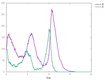
dA/dt = k2 · A − k1 · A · B dB/dt = k1 · A · B − k3 · B and sustained oscillations as shown in Fig. 2.

The stochastic semantics of a reaction network is defined by a transition relation, noted −→S, between discrete states

describing the number of each molecule, i.e. vectors ~x ∈ Ns_.

A transition is enabled if there are enough reactants to fire one reaction. Each reaction is associated with a transition of propensity given by the rate function as follows:

∀(Ri, Ii, Pi, fi), ~x −→fSi ~x0 with propensityfi

if ~x ≥ Riand ~x0= ~x − Ri+ Pi

Transition probabilities between discrete states are ob-tained through normalization of the propensities of all enabled reactions, and the time of next reaction can be computed from the rates à la Gillespie [28]. It is worth noting that in this interpretation, as in the differential semantics, the inhibitors are supposed to decrease the reaction propensity but do not prevent the reaction from occurring. They are

Fig. 2. Sustained oscillations obtained in the differential semantics of Ex. 1 showing very low concentrations ofAperiodically.

Fig. 3. Almost sure extinction of the predator obtained in the stochastic semantics of Ex. 1 due to the periodic decrease to low numbers of molecules.

thus ignored by the stochastic transition enabling conditions similarly to the differential semantics.

In Ex. 1, the stochastic interpretation can exhibit some oscillations similar to the differential interpretation, but almost surely the extinction of the predator, i.e. a qualita-tively different behavior illustrated in Fig. 3, due to the low numbers of molecules which almost surely will go to zero.

The Petri net semantics is defined similarly on discrete states with a transition relation −→D which just ignores

the rate functions and is thus a trivial abstraction of the stochastic semantics by a forgetful functor:

∀(Ri, Ii, Pi, fi), ~x −→D~x0if ~x ≥ Ri, ~x0 = ~x − Ri+ Pi

The Boolean semantics is similar to the Petri net one but on Boolean vectors x of Bs, obtained by the “zero, non-zero” abstraction of integers. With this abstraction, when the number of a molecule is decremented, it can still remain present, or become absent. It is thus necessary to take into account all the possible complete consumption or not of the reactants in order to obtain a correct Boolean abstraction

of the Petri net and stochastic semantics [2]. The Boolean transition system −→Bis thus defined by:

∀(Ri, Ii, Pi, fi), ∀S ≤ Ri, ~x −→B~x0

if ~x ≥ Ri, ~x0 = ~x − S + Pi.

The Boolean trace semantics provides an over-approximation of the qualitative behaviors of the stochastic semantics. As proven in [2], the discrete (i.e. stochasic, Petri net, Boolean) semantics are related by successive Galois connections, which means that, for instance, if a trace is not possible in the Boolean semantics, it is not realizable in the Petri net semantics, whatever the stoichiometric coefficients are, nor in the stochastic semantics, whatever the reaction rates are.

Example 3. Complex Boolean behavioral properties, including

reachability of stable or just steady states (i.e. respectively from which one cannot leave or may not leave) can be expressed in Com-putation Tree Logic (CTL) and automatically verified by model-checking algorithms [29]. In Ex. 1, the enumeration of true CTL formulae of some simple patterns, reveals the possibly steady but not stable persistence of the predator (which can always disappear if the prey becomes extinct), the possible stable persistence of the prey (if the predator becomes extinct), the possible extinction of both the predator and the prey, and the absence of Boolean oscillations: biocham: present({A,B}). biocham: generate_ctl_not. reachable(stable(A)) reachable(stable(not A)) reachable(stable(not B)) reachable(steady(B))

On the other hand, the differential semantics is generally not an abstraction of the stochastic behavior. It has been shown in [30] that if the numbers of all molecules tend to in-finity, the mean stochastic behavior tends to the differential behavior. In Ex. 1, these limit conditions are obviously not satisfied and the mean stochastic behavior is very different from the differential behavior.

2.4 Discrete Semantics with Negation

In the different semantics of the previous section, a reaction inhibitor acts solely on the reaction rate, its presence does not prevent the reaction to proceed. Though not common for reaction networks, contrarily to influence networks studied in the next section, one can also consider discrete (stochastic, Petri net, Boolean) semantics with negation where the set of inhibitors of a reaction is seen as a conjunction of negative conditions for the transition (disjunctions can be represented with several reactions).

In order to express negative conditions on multisets, let us denote by <0 the strict pointwise order between two

multisets restricted to the intersection of their supports. The Boolean with negation transition system −→BN can then be

defined by:

∀(Ri, Ii, Pi, fi)∀S ≤ Ri, ~x −→BN ~x0

if ~x ≥ Ri, ~x <0Ii, ~x0= ~x − S + Pi.

The stochastic and Petri net semantics with negation can be defined similarly just by adding the condition ~x <0 Ii to

the transitions, i.e. the condition of absence of an inhibitor is replaced by an inequality constraint on its number.

It is worth remarking that in the Petri net semantics with negation, the test for absence of species (named inhibitor

arc) makes the formalism Turing complete and reachability undecidable [31]. However, the negative conditions on mul-tisets allow us to implement k-bounded Petri nets, i.e. with a finite state transition graph, simply by adding a reaction inhibitor of the form k · x with some level coefficient bound k to all the reactions that produce x.

2.5 Influence Graph of a Reaction Network

Here we recall two definitions of the influence graph5 asso-ciated with a reaction network, and their equivalence under general assumptions [17], [25]. The first definition is based on the Jacobian matrix J formed of the partial derivatives Jij = ∂ ˙xi/∂xj, where ˙xi is defined by the differential

semantics.

Definition 3. The differential influence graph (DIG) asso-ciated with a reaction network is the graph having for vertices the molecular species, and for edge-set the following two kinds of edges:

{A →+_{B | ∂ ˙x}

B/∂xA> 0 for some value ~x ∈ Rs+}

∪{A →−_{B | ∂ ˙x}

B/∂xA< 0 for some value ~x ∈ Rs+}

Definition 4. Thesyntactical influence graph (SIG) associated with a reaction network M is the graph having for vertices the molecular species, and for edges the following set of positive and negative influences: {A →+_{B | ∃(R} i, Ii, Pi, fi) ∈ M (Ri(A) > 0 and Pi(B) − Ri(B) > 0) or (Ii(A) > 0 and Pi(B) − Ri(B) < 0)} ∪{A →−_{B | ∃(R} i, Ii, Pi, fi) ∈ M (Ri(A) > 0 and Pi(B) − Ri(B) < 0) or (Ii(A) > 0 and Pi(B) − Ri(B) > 0)}

The syntactical graph is trivial to compute, in linear time, by browsing the syntax of the rules.

Example 4. In Ex. 1 both definitions give the same influence

graph:

B

A

Both definitions are equivalent if the syntactical influ-ence graph contains no conflict, i.e. no pair of the form A →+_{B and A →}−_{B between the same molecules:}

Theorem 1( [17], [25]). For any well-formed reaction network (resp. such that the syntactical influence graph contains no con-flict), the differential influence graph is included in (resp. identical to) the syntactical influence graph.

3

I

N

F

In this section, we introduce influence networks with forces and equip them with a hierarchy of differential, stochas-tic, Petri net and Boolean semantics, similarly to reaction networks. We then compare their expressive power with reaction networks, and focus on different variants of their discrete semantics to compare them with Thomas’s setting for gene regulatory networks.

5. By a slight abuse of terminology, we call influence graph a labeled multigraph, since there may be both a positive and a negative influence from one vertex to another one.

3.1 Syntax

The idea to disambiguate the semantics of the different influences incoming on a vertex of the influence graph, is to syntactically distinguish conjunctive from disjunctive con-ditions in an influence network, by writing influences with several sources for representing a conjunction of conditions, while the different influences on a same target express a disjunction of conditions. These syntactical conventions are a particular case of the concept of multiplexes introduced in [32] restricted here to disjunctive normal forms (DNFs).

Definition 5. Given S = {x1, . . . , xs} a set of species, an

influence network I is a set of quintuples (P, I, t, σ, f ) called influences, where

• P is a multiset on S, called positive sources of the

influence,

• I a multiset of negative sources,

• t ∈ S is the target,

• σ ∈ {+, −} is the sign of the influence, accordingly called

either positive or negative influence,

• and f : Rs→ R is a real function called the force of the

influence.

In addition, we distinguish the positive sources from the negative sources in an influence (positive or negative), in order to annotate the fact that in the differential semantics, the source increases or decreases the force of the influence, and in the Boolean semantics with negation whether the source or the negation of the source is a condition for a change in the target.

In the examples below, we use the ASCII syntax of BIOCHAM v4 for influences. Positive (resp. negative) in-fluences are written with an arrow -> (resp. -<) which separates the sources from the target. The positive and negative sources are separated by a /, which can be omitted if there is no negative source.

The concept of well-formed influence networks can be defined similarly to Def. 2 as follows:

Definition 6. An influence (P, I, t, σ, f ) over molecular species

{x1, . . . , xs} is well-formed if the following conditions hold:

1) f (x1, . . . , xs) is a partially differentiable function,

non-negative on Rs +;

2) xi∈ P if and only if σ = + (resp. −) and ∂f /∂xi(~x) >

0 (resp. < 0) for some value ~x ∈ Rs +;

3) xi∈ I if and only if σ = + (resp. −) and ∂f /∂xi(~x) <

0 (resp. > 0) for some value ~x ∈ Rs +;

4) t ∈ P if σ = −.

Example 5. The reaction model of Ex. 1 can also be represented

by the following well-formed influence network: k1*A*B for A,B -< A.

k1*A*B for A,B -> B. k2*A for A->A.

k3*B for B-<B.

composed of four well-formed influences, with positive sources only, ({A, B}, ∅, A, −, k1 · A · B), ({A, B}, ∅, B, +, k1 · A · B), ({A}, ∅, A, +, k2 · A) and ({B}, ∅, B, −, k3 · B). These four influences, two of which contain a conjunction of two sources, are consistent with the six edges of the influence graph depicted in Ex. 4. It is also worth noting that in our setting, one can model

the inhibition of the autocalysis of A by some other variable C, by putting C as negative source in the positive influence rule for A: k2*A/(1+C) for A/C -> A.

i.e. without using a negative influence rule.

3.2 Hierarchy of Semantics

The differential semantics of an influence network I over S, is given by (the solutions of) the following ODE system:

dxk dt = X (Pi,Ii,xk,+,fi)∈I fi− X (Pj,Ij,xk,−,fj)∈I fj

This ODE adds up all the forces of the positive influences on xkand subtracts all forces of negative influences on xkin

the derivative of xk over time. In Ex. 5, one can easily check

that this definition leads to the same equations as for Ex. 1. The negative sources in a well-formed influence decrease the force of the influence but do not disable it. Consequently, we define the stochastic semantics of an influence network with forces, by a transition system, noted −→S, between

discrete states, i.e. vectors ~x of Ns_{, such that an influence}

is enabled if the positive sources are present in sufficient number, no condition on the negative sources, the transition propensity is defined by the force, and the target is updated as follows (by abuse of notation the sign σ is also used in the sequel as increment and decrement operations):

∀(Pi, Ii, ti, σi, fi), ~x −→fSi ~x0with propensityfi

if ~x ≥ Piand ~x0= ~x σiti

As previously for reaction netowkrs, the transition prob-abilities between discrete states are obtained through nor-malization of the propensities of all enabled transitions, and the time of next reaction is computed as in Gillespie’s algo-rithm [28]. The negative sources are supposed to decrease the influence propensity but do not prevent the influence from proceeding.

The Petri net (PN) semantics simply ignores the forces: ∀(Pi, Ii, ti, σi, fi), ~x −→D x~0if ~x ≥ Pi, ~x0 = ~x σi ti It is

worth noting here that since a target has no multiplicity coefficient, a PN or stochastic transition always adds or subtracts one to the level of the target, and cannot define a self-loop in the state transition graph.

The positive Boolean semantics is defined on Boolean vec-tors x of Bs, by the “zero, non-zero” abstraction of integers of the Petri net semantics. Consequently, the Boolean seman-tics associates two transitions with one negative influence: one that inactivates the target, and one that loops with the target active6_:

∀(Pi, Ii, ti, +, fi), ~x −→B ~x0if ~x ≥ Pi, ~x0= ~x + ti

∀(Pi, Ii, ti, −, fi), ~x −→B~x0if ~x ≥ Pi, ~x0 = ~x or ~x0= ~x − ti

This Boolean semantics is positive in the sense that it ignores the negative sources of an influence and contains no nega-tion in the enabling condinega-tion. In Ex. 5, one can check that the Boolean transitions are the same as in Ex. 1, although in general one can expect to get more transitions (Thm. 3.3 and Prop. 1 below).

With these definitions, we obtain as in [2] a hierarchy of semantics related by simple Galois connections between a concrete domain and an abstract domain [18], noted (C, vc)−→

α

←−γ (A, vA), which will be here limited to the

dis-crete semantics domains formalized by set lattices ordered by inclusion.

Theorem 2. For an influence network I, the stochastic

seman-tics, the Petri net semantics and the Boolean semantics are related by Galois connections, ({~x −→fi S ~x0}, ⊆) −→αSD ←−γSD ({~x −→D ~ x0_{}, ⊆)}−→_←−αDB γDB ({~x −→B~x 0_{}, ⊆).}

Proof. Let us first remark that our transition semantics are sets and that in powerset domains, the pointwise extension of any function from the base set of the concrete domain to the abstract domain forms a Galois connection [2]. Thus we just have to define the abstraction functions pointwise to obtain Galois connections with respect to the set inclusion ordering.

The first abstraction of the stochastic semantics by the Petri net semantics is a trivial abstraction by a forgetful functor αSD, namely the erasing of the propensities in the

transitions.

The second abstraction αDB abstracts discrete states

by Boolean states. The domain of Boolean transitions is related to the Petri net transitions semantics domain by the zero/non-zero abstraction from the integers to the Booleans, αN B : N → B, and its pointwise extension from discrete

states to Boolean states.

We can easily check that the Boolean transitions are indeed the abstraction by αN Bof the Petri net transitions. In

particular for a negative influence, the transition ~x0= ~x − ti

in the integer vector domain, is abstracted in the Boolean vector domain by the zero/non zero abstraction with the two transitions ~x0= ~x or ~x0 = ~x − ti.

Corollary 1. If a behavior is not possible in the positive Boolean

semantics of an influence network, it is also not possible in the Petri net and stochastic semantics for any forces.

3.3 Expressive Power

Let us first show that an influence network can always be simulated by a reaction network.

Theorem 3. Any (well-formed) influence network with forces can

be represented by a (well-formed) reaction network, with the same Boolean, Petri net, stochastic and differential semantics.

Proof. Let us represent a positive influence (P, I, t, +, f ) by a catalytic synthesis reaction (P, I, P ] {t}, f ). Similarly, let us represent a negative influence (P, I, t, −, f ), by an active degradation reaction (P ] {t}, I, P, f ). It is straight-forward to verify that the Boolean, Petri net, stochastic as well as differential semantics recalled and defined above are the same. Furthermore, the well-formedness condition is preserved. Indeed, this property only depends on the forces/rate functions and on the reactants/inhibitors, which do not change through that transformation thanks to the condition that in well-formed influence networks, the target of a negative influence must be a positive source t ∈ P .

Interestingly, the converse of this theorem holds for the differential semantics with all generality:

Theorem 4. Under the differential semantics, (well-formed)

in-fluence and reaction networks have the same expressive power. Proof. For each reaction (R, I, P, f ) of a given reaction net-work, let us add the following influences:

(R, I, xi, +, (P (i) − R(i)) · f ) when P (i) − R(i) > 0

(R, I, xi, −, (R(i) − P (i)) · f ) when P (i) − R(i) < 0

The associated ODE system collects all (Pi− Ri) · f

ex-actly as in the differential semantics of the original reaction network. Furthermore, it is easy to check that these influ-ences are formed since the original reaction is well-formed and the force is only a positive integer multiplied by the original rate function.

This theorem shows that as far as the differential se-mantics is concerned, the influence networks have the same expressive power as reaction networks and there is no theoretical reason to develop a reaction model. Con-versely, using [25] one can define some canonical reac-tion network corresponding to an influence network by inferring it from the differential semantics. Note however that for instance starting from the self-negative influence (X, ∅, X, −, kX2_{) one obtains ˙X = −kX}2 _{and therefore}

the reaction ({X}, ∅, ∅, kX2_{) and not ({2X}, ∅, {X}, kX}2_).

Both have the same differential semantics, the second obeys Mass-Action and not the first, and their discrete semantics will differ (e.g., when there is only one X).

The converse of Thm. 3 does not hold for the Boolean, Petri net or stochastic semantics. Indeed, in those se-mantics the (well-formed) reaction of mutual degradation ({A, B}, ∅, ∅, k.A.B) defines a transition from the state (A, B) = (1, 1) to (0, 0) which is obviously not possible in an influence network since only one variable can change in one transition. Note that it is not obvious to associate an influence network, even simply to simulate the reaction network behavior. For instance, the influence network ob-tained from our mutual degradation’s differential semantics would consist of the two influences ({A, B}, ∅, A, −, k.A.B) and ({A, B}, ∅, B, −, k.A.B). However from state (1, 1) it is actually impossible to reach (0, 0). One would need to add self-negative-loops on both A and B, which would lead to a quite crude over-approximation.

Let us call a reaction (R, I, P, f ) unitary if the support of P − R is a singleton with a result equal to either 1 or −1.

Proposition 1. Any (well-formed) network of unitary reactions

can be represented by a (well-formed) influence network with the same Boolean, Petri net, and stochastic semantics.

Proof. Let us associate with each unitary reaction (R, I, P, f ), with P (t) − R(t) = ±1 and P (x) = R(x) for all x 6= t, the influence (R, I, t, σ, f ) where σ is the sign of P (t) − R(t).

The stochastic and Petri net transitions associated with the unitary reaction (R, I, P, f ) apply on discrete states satisfying ~x ≥ R and ~x0 = ~x − R + P = ~xσt, i.e. the same transitions as for the influence (R, I, t, σ, f ).

The Boolean transitions associated with the unitary re-action (R, I, P, f ) apply on discrete states satisfying ~x ≥ R and ~x0= ~x − S + P for all S ≤ R.

If P (t) − R(t) = −1 then either ~x0 = ~x or ~x0= ~x − t. Therefore in both cases, the Boolean transitions associ-ated with the reaction (R, I, P, f ) are the same as those associated with the influence (R, I, t, σ, f ).

3.4 Semantics with Negation

Contrarily to reaction networks, it is usual in Boolean in-fluence networks and regulatory networks à la Thomas, to adopt a strict interpretation of the negative sources of an influence, as tests for absence of those species in the enabling condition. This choice is made at the expense of losing the relationships to the differential semantics, and to the (positive) stochastic and Petri net semantics (Thm. 2) since, for instance, a positive influence like A/2B → C can activate C with B present at level 1 in the Petri net semantics, but not in the Boolean semantics which is thus no longer an abstraction of the Petri net semantics.

Formally, the Boolean with negation semantics of an influ-ence network is defined by the following transition system:

∀(Pi, Ii, ti, σi, fi), ~x −→BN~x0

if ~x ≥ Pi, ~x <0Ii, ~x0= ~x σiti

Then, one can also define stochastic and Petri net seman-tics with negation by adding the condition ~x <0 Ii on the

negative sources to the transition, as done in Sec. 2.4 for the reaction networks, but with a similar loss of connection to the differential semantics.

As already remarked for reaction networks, this strict interpretation of the negative sources makes it possible to express influence networks with bounded multi-level seman-tics, simply by adding a negative source k · x to all the positive influences on x, with some level coefficient bound k. This is adopted in tools such as GINsim [9], [10], but is not possible in the positive semantics of the previous section.

That interpretation of negative sources by negation in-creases the expressive power of influence networks. Let us call a unitary transition system, a transition system that updates at most one variable of ~x in each transition7_{. An} influence network always defines such a unitary transition system under the discrete semantics, since the target t is a single species.

Proposition 2. Any unitary Boolean transition system can be

represented by an influence network under the Boolean semantics with negation.

Proof. It is sufficient to notice that since a unitary Boolean transition s −→BN s0 changes at most one species, say ti,

from s to s0, it can be represented by

• either a positive influence, (P, I, ti, +), if s0(ti) = 1, • or a negative influence, (P, I, ti, −), if s0(ti) = 0,

with P = {x | s(x) = 1} and I = {x | s(x) = 0}.

3.5 Functional Semantics à la Thomas

The Boolean and multi-level semantics defined by René Thomas originally for gene networks [6], is functional, in the sense that the next state ~x0 _{is defined by a}

func-tion φ(~x) of the previous state, not a relation. In this

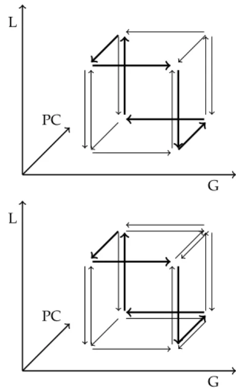
7. It is worth remarking that in a unitary transition system, the state transition graph lives on a hypercube (e.g. Fig. 7 in Sec. 5 below).

setting, the synchronous semantics is deterministic, and the non-deterministic asynchronous semantics is obtained by interleaving, by considering all the possible transitions that change the value of exactly one of the genes at a time. A truly non-deterministic influence network such as {(A, ∅, B, +, f ), (A, ∅, B, −, g)}, for which the transition relation is not a function, cannot be represented. For this reason Thomas’s setting excludes self-loops in the state transition graph and all steady states are stable (i.e. terminal states).

Proposition 3. The set of Boolean transition systems definable

by Thomas’s regulatory networks is the set of unitary Boolean transition systems without self-loops.

Proof. A Thomas’s transition graph is necessarily unitary and without self-loops since each transition changes the Boolean value of exactly (not at most) one variable at a time. The converse follows from Prop. 2 by excluding the possibility of having self-loop transitions which change no variable.

Corollary 2. Any Thomas’s regulatory network N can be

repre-sented by an influence network under the Boolean semantics with negation.

Proof. From Prop. 3 N is unitary, one can therefore apply the encoding of the proof of Prop. 2 to obtain a correspond-ing influence network (note that in practice much smaller influence networks can be obtained by considering the DNF of the activation functions).

The restriction to functional transitions is even more striking in Thomas’s multi-level setting, where the above system can (in the discrete semantics) have transitions from (1, 1) both to (1, 0) and to (1, 2). That would necessitate the corresponding logical parameter for B to be at the same time < 1 and > 1. It is worth noting that despite this subtle restriction in the expressive power, the logical formalism of Thomas is successfully used in a wide variety of models [23], [33], [34], [35] in systems biology.

3.6 Influence Graph of an Influence Network

The differential influence graph of an influence network is defined though the differential semantics, as in Def. 3. We get a similar equivalence result with the following syntacti-cal definition of the influence graph:

Definition 7. Thesyntactical influence graph (SIG) associated with an influence network I is the graph having for vertices the molecular species, and for edges the following set of positive and negative influences: {A →+_{B | ∃(P} i, Ii, B, σi, fi) ∈ I (A ∈ Piand σi= +) or (A ∈ Iiand σi= −)} ∪{A →−_{B | ∃(P} i, Ii, B, σi, fi) ∈ I (A ∈ Piand σi= −) or (A ∈ Iiand σi= +)}

Proposition 4. For a well-formed influence network such that the

syntactical influence graph contains no conflict, the syntactical and differential influence graphs are identical.

˙ xB= X (Pi,Ii,xB,+,fi)∈I fi− X (Pj,Ij,xB,−,fj)∈I fj ∂ ˙xB ∂xA = X (Pi,Ii,xB,+,fi)∈I ∂fi ∂xA − X (Pj,Ij,xB,−,fj)∈I ∂fj ∂xA

Since the SIG does not have any conflict, A →+ B is in the SIG if and only if

∂ ˙xB ∂xA = X (Pi,Ii,xB,+,fi)∈I,A∈Pi,A6∈Ii ∂fi ∂xA − X (Pj,Ij,xB,−,fj)∈I,A6∈Pj,A∈Ij ∂fj ∂xA

and a similar reasoning can be made for A →− B. Now, since the influence network is well-formed, all terms of the left-hand sum are non-negative (A 6∈ Ii) and

strictly positive for some points ~xi.

Similarly, all terms of the right-hand sum are non-positive (A 6∈ Pj) and strictly negative for some ~xj.

We have that A →+_{B in the SIG iff the above sum has at}

least one term, that is equivalent to the existence of some ~x in the state space where one of the terms above is non-null, in which case∂ ˙xB

∂xA

> 0, i.e., A →+_{B is in the DIG.}

Furthermore, one can easily check that in the representa-tion of an influence network by a reacrepresenta-tion network (Thm. 3), the influence graphs associated with them are the same.

4

P

P

S

C

B

A

In this section, we focus on the positive Boolean semantics of influence networks and study its properties. In partic-ular, we show that the Boolean attractors of the positive semantics contain the attractors of the functional semantics with negation à la Thomas and provide an efficient pruning algorithm for computing them. Let us recall that ≤ denotes the pointwise order on {0, 1} coordinates of vectors repre-senting states.

Proposition 5(Monotonicity). The positive Boolean semantics of influence networks is monotonic: let I be an influence network over S = {x1, . . . , xs} and v1, v2 be two Boolean states, i.e.,

vectors of Bs if v1≤ v2then ∀v10, v1−→ v01, ∃v 0 2, v 0 1≤ v 0 2and v2−→ v02 v1 v2 v10 v₂0 ≤ ≤

Proof. One can simply notice that since there are no nega-tions in the enabling condinega-tions, any influence that is en-abled in v1is also enabled in v2.

It is worth noticing that this monotonicity property for transitions is fundamentally different from that of monotone dynamical systems [36] which are deterministic, and there-fore impose the monotonicity property on the unique image of v1 and v2. In our setting, Prop. 5 states that there exists

some v20 ≥ v10, but the existence of negative influences in the

network permits that some other images of v2might not be

greater than v01. Nevertheless, we have

Proposition 6 (Greatest element). Let C be a Terminal Strongly Connected Component (TSCC) of the state transition graph of a positive influence network, then C has a greatest element: ∃v0∈ C, ∀v ∈ C, v ≤ v0

Proof. Let us prove this proposition by contradiction: as-sume that there are two incomparable maximal elements v1and v2in C.

Since C is strongly connected there is a path from v1 to

v2 and along that path a state v3 and its successor in the

path v4such that v3≤ v1and v46≤ v1, as v26≤ v1.

Now, using Prop. 5 we get that v1 −→ v01with v4 ≤ v10

and v10 ∈ C since C is terminal.

However, v10 is either greater or less than v1since it is the

result of applying a single influence.

If v1 < v01 we have a contradiction as we supposed v1

maximal.

If v10 ≤ v1we get v4≤ v1by transitivity and that is also

contradictory.

Corollary 3. To enumerate the attractors, i.e., TSCCs, of a

positive influence network, it is enough to check the strongly connected components (SCCs) of states that have no strictly increasing transition.

Proof. This is an immediate consequence of Prop. 6 as each TSCC can be represented by its greatest element which has no strictly increasing transition.

Notice that stable states are a particular case with no strictly decreasing transition either. Moreover, any strictly decreasing transition should be “reversible” for the SCC to be a TSCC. This allows us to rule out potential TSCC candidates without exploring their whole SCC in Alg. 1 and Alg. 2 (implementation available in BIOCHAM v4).

Note that in Alg. 2 two temporal logic formulae are used: the first one checks that from any state reachable by C, C remains always (AG) reachable (EF (C)), the second one is the previous one about reachability to ensure that no stable state S is reachable (¬EF (S)) from C.

Proposition 7. Let I be an influence network, there is at least

one TSCC of its state transition graph in each TSCC of its positive semantics’ state transition graph.

Proof. The positive semantics only adds transitions by enabling more influences, it can therefore only merge TSCCs.

This result suggests finding complex attractors of non-positive networks, such as logical models à la Thomas [7], [8] that are particular cases of influence networks (see Cor. 2), by enumerating the greatest elements of the TSCCs of their positive Boolean semantics, and then looking for attractors of the original network. This approach provides an over-approximation of the attractors and is complementary to recent works which provide lower-bounds on their num-ber [37].

One might note however that the reversibility constraint on decreasing transitions can easily be stated as a constraint of our Constraint Satisfaction Problem (CSP). Now, check-ing that an SCC is terminal can be done through model

Algorithm 1TSCC maximal elements candidates enumera-tion algorithm

procedureLIST_TSCC_CANDIDATES

Constraints ← {P ∧ ¬I =⇒ t | (P, I, +, t, f ) ∈ I} . Enabled positive influences must not change the state

Candidates ←ENUMERATESOLUTIONS(Constraints)

for C ∈ Candidates do

if Chas no strictly decreasing transition then C is a stable steady state

else if C has a non-reversible strictly decreasing transition then

C is not in a TSCC

else

C’s SCC must be explored to check if it is a TSCC

end if end for end procedure

functionENUMERATESOLUTIONS(Constraints)

Iteratively solve by SAT/CP the Constraint Satisfac-tion Problem (CSP) defined by Constraints

returnThe set of solutions

end function

checking, and verifying if there is a singular TSCC inside a positive TSCC is also a reachability problem. Putting all this together we reach a refined version, Alg. 2 of our original algorithm, Alg. 1 that now guarantees that an SCC it finds is terminal, and also checks for inclusion of stable states. Alg. 2 therefore provides a lower bound on the number of complex attractors, and an over-approximation of those.

5

E

E

The following examples from the literature illustrate the links between reaction and influence networks (mostly Thm. 4), the encoding of Thomas’s networks as influence networks (Cor. 2), and the use of the positive semantics and Alg. 2 to efficiently enumerate the complex attractors of an influence network. In particular in the third example, our algorithm enumerates the attractors in 106s, whereas the algorithms based on the construction of the transition graph, such as implemented in GINsim [9], [10], fail by out of memory.

The CPU times are given in seconds and have been obtained on a Macbook Pro, as all the CPU times given in this paper.

5.1 Influence Model of the p53/Mdm2 DNA Damage Re-pair System [20]

The p53/Mdm2 DNA damage repair system is an inter-esting oscillatory system which has been modeled by dif-ferential equations by Ciliberto et al. in [27]. Fig. 1 shows the reaction network. Note that this model contains explicit transport reactions of Mdm2 between the cytoplasm and the nucleus, and that p53 is an inhibitor of the phosphorylation reaction of Mdm2 in the cytoplasm (Ex. 2). Fig. 4 shows the influence graph of this reaction model, as given by Def. 4).

In [20], a simplified regulatory model à la Thomas was manually derived from the reaction model of [27], and

Algorithm 2Refined TSCC search algorithm

procedureLIST_TSCC_CANDIDATES

Stable ← ENUMERATESTABLE()

Constraints ← {P ∧ ¬I =⇒ t | (P, I, +, t, f ) ∈ I} . Enabled positive influences must not change the state

Constraints ← Constraints ∪ {P ∧ ¬I =⇒ t ∨ W

iPi∧ ¬Ii| (P, I, −, t, f ), (Pi, Ii, +, t, fi) ∈ I, t 6∈ Pi}

. Enabled negative influences must be reversible Candidates ←ENUMERATESOLUTIONS(Constraints)

for C ∈ Candidates do if C ∈ Stable then

C is a stable steady state

else if C 6|= AG(EF (C))(positive semantics) then C is not in a TSCC

else

C is in a positive TSCC

if ∀S ∈ Stable, C |= ¬EF (S) (negative se-mantics) then

there is at least one negative non-trivial TSCC (a complex attractor) in C’s TSCC

end if end if end for end procedure

functionENUMERATESTABLE

Iteratively solve by SAT/CP the CSP corresponding to the absence of state-changing enabled influence

returnThe set of solutions

end function

functionENUMERATESOLUTIONS(Constraints)

Iteratively solve by SAT/CP the CSP defined by Constraints

returnThe set of solutions

end function

analyzed with logical semantics. Fig. 5 shows the influence graph of their model. Here, we first give a formal derivation of this influence graph using the definitions of this paper, and then illustrate the search for TSCCs in the correspond-ing Boolean influence network.

When comparing the influence graphs of the reaction model of [27] (Fig. 4) with the simplified influence model of [20] (Fig. 5), one can remark that the simplified graph can be essentially obtained by

• merging p53 and p53u in P,

• deleting p53uu,

• merging Mdm2pc and Mdm2n in N,

• and renaming Mdm2c in C and DNAdam in D. Such operations correspond to the notion of subgraph epi-morphism (SEPI) and SEPI-reduced models studied in [38]. Fig. 6 shows the influence graph (Def. 4) of the SEPI-reduction of the original reaction model obtained with the operations above. The only differences with Fig. 5 are the absence of the negative self-loops, and of the positive influ-ence from N to C corresponding to the transport of Mdm2 from the nucleus to the cytoplasm, which were neglected in [20].

In addition to the influences represented by this influ-ence graph, the logical model of [20] considers the

tran-p53 p53u DNAdam Mdm2c Mdm2pc Mdm2n p53uu

Fig. 4. Influence graph (Def. 4) of the reaction model of [27] (Fig. 1).

C N

P D

Fig. 5. Simplified influence graph displayed in Fig. 4 of [20], without the activation multi-levels.

sitions to basal states, i.e. attractive states in absence of other influences, for the activation of p53 (_ -> P) and DNA-damage (_ -> D), and the degradation of cytoplas-mic Mdm2 (C -< C). This leads to the following influence networks and computation of attractors, without and with the basal influences.

biocham: P -> C. C -> N. N -< P. P -< N. P -< D. D -< N. biocham: list_tscc_candidates. [C-0,D-0,N-0,P-0] stable [C-0,D-0,N-1,P-0] stable [C-0,D-1,N-0,P-0] stable [C-1,D-0,N-1,P-0] stable [C-1,D-1,N-1,P-0] terminal (positive) P D C N

Fig. 6. Influence graph (Def. 4) of a SEPI reduction [38] of the reaction model of [27].

contains a complex attractor Candidates from constraints: 1 Complex TSCCs computed: 1 Time: 0.026

biocham: _ -> P. _ -> D. C -< C. biocham: list_tscc_candidates.

[C-1,D-1,N-1,P-1] terminal (positive) contains a complex attractor

Candidates from constraints: 1 Complex TSCCs computed: 1 Time: 0.015

Alg. 2 shows that even with a Boolean model, where P acts simultaneously on C in a negative cycle, and N in a positive cycle, there is a single complex attractor, similarly to the results of the complete analysis of [20] using a multi-level model. The algorithm also finds four stable steady states in absence of the basal influences.

Furthermore, the extension of that model with differen-tial and stochastic dynamics studied in [21] could be directly represented by influence forces in this setting.

5.2 Influence Model of the Mammalian Circadian Clock [22]

Another nice example of the use of logical models à la Thomas is the article by Comet et al. [22] studying different variants of small models of the circadian rhythms in mam-mals. They derive a small influence network à la Thomas, from the following 4-variable ODE model, which is itself a simplified version of the 16-variable model from [39]:

dPC dt = Kn Kn_{+ P C}n N v1− k3PCCC+ k4P CC− kd1PC dCC dt = Kn Kn_{+ P C}n N v2− k3PCCC+ k4P CC− kd2CC dP CC dt = k3PCCC− k4P CC− k1P CC+ k2P CN− kd3P CC dP CN dt = k1P CC− k2P CN− kd4P CN

The reaction network corresponding to those ODEs [25] is: kd1*PC for PC => _. kd2*CC for CC => _. kd3*PCC for PCC => _. kd4*PCN for PCN => _. k1*PCC for PCC => PCN. k2*PCN for PCN => PCC. k3*PC*CC for PC + CC => PCC. k4*PCC for PCC => PC + CC. K^n*v1/(K^n + PCN^n) for _ / PCN => PC. K^n*v2/(K^n + PCN^n) for _ / PCN => CC.

As per Thm. 4, one obtains an influence network with the same differential semantics. In the small logical model of [22], the authors further simplify the Per and Cry proteins (P C is their complex, G their genes) and introduce light (L) in order to study light entrainment. The obtained model though very small remains quite useful, since it provides a causal explanation of the robustness of the circadian clock to variations of day length.

A direct import in BIOCHAM v4 of their logical model without delays (cf. Section 5 of [22]) gives the following influence network with negative sources, shown below with the corresponding influence graph:

_ / L -> L. L -< L. _ / G, PC -> G. G, PC -< G. G / PC, L -> PC. PC / G -< PC. PC, L -< PC. L PC G

Fig. 7 shows that the positive semantics of this network is close to the original Boolean semantics with negation à la Thomas of the model. Only a few state transitions become reversible in the positive Boolean semantics, while they are irreversible in the original Boolean semantics with negation à la Thomas of the model.

Furthermore, both the positive and negative Boolean semantics have a single TSCC, namely the whole state transition graph represented by the vector (1, 1, 1) found as sole candidate:

biocham: list_tscc_candidates. [G-1,L-1,PC-1] terminal (positive) contains a complex attractor

Candidates from constraints: 1 Complex TSCCs computed: 1 Time: 0.016

The approximation introduced by the positive Boolean semantics can also be explained by quantitative dynamics considerations. For instance, when G is on, the transcription leading to the PER-CRY complexes is stimulated, how-ever [22] explains that these complexes can only migrate to the nucleus in absence of light. This absence cannot be checked in a positive semantics model, however the consen-sus mechanistic process is rather thought to be a modulation of PER transcription by light (see for instance [39] for the mammalian case). Being purely quantitative, it is not easy to take into account such a regulation in a Boolean model except with the reversible activation of P C when G is on,

G L PC G L PC

Fig. 7. State transition graphs of the model under, the Boolean se-mantics with negation à la Thomas, similar to Fig. 7 of [22] (top), and the positive Boolean semantics, where some state transitions have become reversible (bottom). The bold circuit represents the classical 24h day-night cycle that is obtained as standard cycle when delays are introduced. The other transitions correspond to recovery pathways in a jet lag context for instance.

whether L is on or not. This is what happens in our positive model as can be seen in the bottom panel of Fig. 7, and it is similar to what happens for the light in the original model.

The same reasoning explains the reversible inactivation of G when P C is active. Indeed there is a basal synthesis of G that cannot check, in a positive setting, that P C is inactive in order to activate the genes. Once again, the mech-anistic process is a quantitative inhibition of the CLOCK-BMAL1 complexes by PER-CRY and a conservative Boolean approximation of that process is reflected by the reversible activation of G in presence of P C.

5.3 Influence Model of MAPK Signaling Network in Uri-nary Bladder Cancer [23]

As a more challenging example, we present here the appli-cation of our methods on a logical model of the influence of Mitogen Activated Protein Kinase (MAPK) signaling in urinary bladder cancer, presented in [23]. Starting, once again, from a “comprehensive reaction map” of 232 species, the authors design a reduced logical model in Thomas’s framework. This 53-variable model, also used as benchmark in [37], describes the influence of the MAPK cascade (and of its inputs, like EGFR over-expression and FGFR3 activating mutation) on cell-fate decision in urinary bladder cancer. As can be seen from Fig. 8 even the reduced model is much bigger than previous examples.

Trying to find attractors with GINsim [9], [10] results in a failure by out of memory after about 1h of computation since it relies on the generation of the full state space. Alg. 2 gives the following results, with a total runtime of 43s:

Fig. 8. Influence graph of the regulatory network à la Thomas of MAPK signaling in urinary bladder cancer [23] as displayed by GINsim.

• 12 steady-states are found. These are the most im-portant features of the model for its original publi-cation (cell-fate) and are easy to find whatever the method (Decision Diagrams in GINsim, Answer Set Programming in [37] and SAT or CSP for us).

• there are 21 states without any strictly increasing

outgoing transition found by constraint solving;

• of those, 15 are in terminal SCCs, as proven by a single call to a model checker;

• and of those TSCCs, only 9 contain one of the pre-viously found steady-states, leading to at least 6 complex attractors.

It is worth noting that the potential cyclic attractors enumerated by our algorithm are of specific interest in this example, since a model of cell-fate decision is not supposed to display such oscillatory behavior.

5.4 Related work

The enumeration of complex attractors in logical and multi-level influence networks by building the state transition graph explicitly cannot work for large networks, as illus-trated in the previous example. There has been recent work on using abstractions to guide the search and prune the search space, somewhat similarly to our approach based on the positive semantics abstraction. In [37], [40] the au-thors describe an algorithm based on the notion of “trap spaces” implemented in the tool PyBoolNet. Their iterative algorithm basically computes the set of minimal trap spaces

using answer set programming (ASP), and checks by CTL model checking (using NuSMV) whether each minimal trap space contains exactly one attractor. The verification by model checking can be very long; however, the computation of minimal trap spaces by ASP is very fast and provides a lower bound on the number of attractors. In the previous example, PyBoolNet finds the same bound as us in less than 1s, but then takes 928s (Core 2 Duo T6670 @ 2.2 GHz, 4 GB) to verify all trap spaces. Our computation of attractors in the positive semantics takes 46s but they are exact and can therefore be studied in a mechanistic view of the model.

6

C

In this paper, we hope to have clarified some differences between influence networks and reaction networks, and especially some subtle discrepancies between the precise Boolean semantics that have been considered in the liter-ature for both kinds of qualitative modeling formalisms. As far as the modeling of one biological system is concerned, a modeler can work with one formalism and one tool to investigate his/her questions about the system. Neverthe-less, as soon as different modeling tools are to be used, or the model has to be communicated and reused or cou-pled to another one for another purpose, understanding and mastering these discrepancies in the semantics of the interactions become crucial.

We have introduced a general formalism of influence networks with forces, and possibly inhibitors, and

devel-oped for it a hierarchy of differential, stochastic, multi-level and Boolean semantics, similarly to reaction networks.

We have first shown that reaction networks and in-fluence networks have the same expressive power under the differential semantics. This means that, as far as the differential equations are concerned, the details given in the reactant-product structure of a reaction network are not necessary, and that the same differential equations can be derived from an influence network with forces.

On the other hand, influence networks have an expres-sive power weaker than reaction networks in the discrete semantics, since they can only express unitary transition systems, i.e. with only one update at a time. Furthermore, the differential semantics in which the inhibitors simply decrease the force without preventing the influence from occurring, lead us to consider positive discrete semantics in which the inhibitors are not interpreted by a negation for testing their absence, but are ignored in the enabling conditions of the influences. This convention ensures that all discrete behaviors are approximated when we go up in the abstractions of the hierarchy of semantics, and that if a behavior is not possible in the positive Boolean semantics (which can be checked by model-checking methods for instance) it is not possible in the stochastic semantics for any forces. On the other hand, we have shown that the Boolean semantics with negation lead to a more expressive formalism, in which any unitary Boolean transition system can be encoded, and for which a similar hierarchy of discrete semantics with negation can also be developed, but with no consistent link to the differential semantics.

Furthermore, we have shown that in the positive Boolean semantics, the monotonicity of the transition rela-tion allows us to enumerate complex attractors efficiently by restricting the search to the greatest elements candidates. The Boolean semantics with negation à la Thomas, contains a restriction on the definition of the transition relation by a function, as opposed to a relation, which limits the sources of non-determinism. With the functional restriction, we have proven that each terminal strongly connected component of the transition graph (TSCC) in the positive semantics contains at least one TSCC of the semantics à la Thomas, and thus that our TSCC computation algorithm can be used to prune the search space in this setting also. On examples from the literature, we have shown that this pruning mecha-nism, similarly to the trap-set approximation of [37], allows us to enumerate attractors where algorithms based on the construction of the transition graph fail.

A

We are grateful to Paul Ruet and Denis Thieffry for in-teresting discussions on Thomas’s framework, to Hannes Klarner and Stalin Muñoz for help in using PyBoolNet, and to the reviewers for their comments. This work was partially supported by ANR project Hyclock under contract ANR-14-CE09-0011, and PASPA-DGAPA-UNAM, Conacyt grants 221341 and 261225.

R

[1] M. Hucka et al., “The systems biology markup language (SBML): A medium for representation and exchange of biochemical

network models,” Bioinformatics, vol. 19, no. 4, pp. 524–531, 2003. [Online]. Available: http://sbml.org/

[2] F. Fages and S. Soliman, “Abstract interpretation and types for systems biology,” Theoretical Computer Science, vol. 403, no. 1, pp. 52–70, 2008. [Online]. Available: http://lifeware.inria.fr/~fages/ Papers/FS07tcs.pdf

[3] N. le Novère, B. Bornstein, A. Broicher, M. Courtot, M. Donizelli, H. Dharuri, L. Li, H. Sauro, M. Schilstra, B. Shapiro, J. L. Snoep, and M. Hucka, “BioModels Database: a free, centralized database of curated, published, quantitative kinetic models of biochemical and cellular systems,” Nucleic Acid Research, vol. 1, no. 34, pp. D689–D691, Jan. 2006.

[4] L. Glass and S. A. Kauffman, “The logical analysis of continuous, non-linear biochemical control networks,” Journal of theoretical Biology, vol. 39, no. 1, pp. 103–129, 1973.

[5] R. Thomas, “Boolean formalisation of genetic control circuits,” Journal of Theoretical Biology, vol. 42, pp. 565–583, 1973.

[6] R. Thomas and R. D’Ari, Biological Feedback. CRC Press, 1990. [7] E. Remy, P. Ruet, and D. Thieffry, “Graphic requirements for

multi-stability and attractive cycles in a boolean dynamical framework,” Advances in Applied Mathematics, vol. 41, no. 3, pp. 335–350, 2008. [8] P. Ruet, “Local cycles and dynamical properties of boolean

net-works,” Mathematical Foundations of Computer Science, vol. 26, no. 4, pp. 702–718, 2016.

[9] A. Naldi, D. Berenguier, A. Fauré, F. Lopez, D. Thieffry, and C. Chaouiya, “Logical modelling of regulatory networks with GINsim 2.3,” Biosystems, vol. 97, no. 2, pp. 134–139, 2009. [10] C. Chaouiya, A. Naldi, and D. Thieffry, Logical Modelling of Gene

Regulatory Networks with GINsim., ser. Methods in molecular biol-ogy (Methods and Protocols). New York, NY: Springer-Verlag, 2012, vol. 804, pp. 463–479.

[11] G. Batt, B. Besson, P. Ciron, H. de Jong, E. Dumas, J. Geiselmann, R. Monte, P. Monteiro, M. Page, F. Rechenmann, and D. Ropers, “Genetic Network Analyzer: a tool for the qualitative modeling and simulation of bacterial regulatory networks,” in Bacterial Molecular Networks. Springer, 2012, pp. 439–462.

[12] D. A. Rosenblueth, S. Muñoz, M. Carrillo, and E. Azpeitia, “In-ference of Boolean networks from gene interaction graphs using a SAT solver,” in AlCoB 2014: Proceedings of the 1st International Conference on Algorithms for Computational Biology, ser. Lecture Notes in BioInformatics, vol. 8542. Springer-Verlag, 2014, pp. 235–246.

[13] C. Chaouiya, “Petri net modelling of biological networks,” Brief-ings in Bioinformatics, vol. 8, no. 210, 2007.

[14] B. Chazelle, “Natural algorithms and influence systems,” Commu-nications of the ACM, vol. 55, no. 12, pp. 101–110, Dec. 2012. [15] A. Naldi, R. Remy, D. Thieffry, and C. Chaouiya, “A reduction

method for logical regulatory graphs preserving essential dynam-ical properties,” in CMSB’09: Proceedings of the seventh international conference on Computational Methods in Systems Biology, ser. Lecture Notes in BioInformatics, vol. 5688. Springer-Verlag, 2009, pp. 266–280.

[16] N. le Novere, M. Hucka, H. Mi, S. Moodie, F. Schreiber, A. Sorokin, E. Demir, K. Wegner, M. I. Aladjem, S. M. Wimalaratne, F. T. Bergman, R. Gauges, P. Ghazal, H. Kawaji, L. Li, Y. Matsuoka, A. Villeger, S. E. Boyd, L. Calzone, M. Courtot, U. Dogrusoz, T. C. Freeman, A. Funahashi, S. Ghosh, A. Jouraku, S. Kim, F. Kolpakov, A. Luna, S. Sahle, E. Schmidt, S. Watterson, G. Wu, I. Goryanin, D. B. Kell, C. Sander, H. Sauro, J. L. Snoep, K. Kohn, and H. Kitano, “The systems biology graphical notation,” Nature Biotechnology, vol. 27, no. 8, pp. 735–741, Aug. 2009.

[17] F. Fages and S. Soliman, “From reaction models to influence graphs and back: a theorem,” in Proceedings of Formal Methods in Systems Biology FMSB’08, ser. Lecture Notes in Computer Science, no. 5054. Springer-Verlag, Feb. 2008. [Online]. Available: http://lifeware.inria.fr/~fages/Papers/FS08fmsb.pdf

[18] P. Cousot and R. Cousot, “Abstract interpretation: A unified lattice model for static analysis of programs by construction or approximation of fixpoints,” in POPL’77: Proceedings of the 6th ACM Symposium on Principles of Programming Languages. New York: ACM Press, 1977, pp. 238–252, Los Angeles.

[19] A. Ciliberto, F. Capuani, and J. J. Tyson, “Modeling networks of coupled enzymatic reactions using the total quasi-steady state approximation,” PLOS Computational Biology, vol. 3, no. 3, p. e45, Mar. 2007.

[20] W. Abou-Jaoudé, D. A. Ouattara, and M. Kaufman, “From struc-ture to dynamics: frequency tuning in the p53–Mdm2 network: I.