HAL Id: hal-01503888
https://hal.univ-lorraine.fr/hal-01503888
Submitted on 13 Dec 2019
HAL is a multi-disciplinary open access
archive for the deposit and dissemination of
sci-entific research documents, whether they are
pub-lished or not. The documents may come from
teaching and research institutions in France or
abroad, or from public or private research centers.
L’archive ouverte pluridisciplinaire HAL, est
destinée au dépôt et à la diffusion de documents
scientifiques de niveau recherche, publiés ou non,
émanant des établissements d’enseignement et de
recherche français ou étrangers, des laboratoires
publics ou privés.
Identification of sub-grains and low angle boundaries
beyond the angular resolution of EBSD maps
Lionel Germain, D. Kratsch, M. Salib, Nathalie Gey
To cite this version:
Lionel Germain, D. Kratsch, M. Salib, Nathalie Gey. Identification of sub-grains and low angle
boundaries beyond the angular resolution of EBSD maps. Materials Characterization, Elsevier, 2014,
98, pp.66-72. �10.1016/j.matchar.2014.10.007�. �hal-01503888�
Identi
fication of sub-grains and low angle boundaries beyond the angular
resolution of EBSD maps
L. Germain
a,b,⁎
, D. Kratsch
c, M. Salib
a,b,d, N. Gey
a,ba
Laboratoire d'Etude des Microstructures et de Mécanique des Matériaux (LEM3), UMR 7239, CNRS/Université de Lorraine, F-57045 Metz, France
bLaboratory of Excellence on Design of Alloy Metals for low-mAss Structures (‘LabEx DAMAS’), Université de Lorraine, France c
Laboratoire d'Informatique Théorique et Appliquée (LITA), EA3079, Université de Lorraine, 57045 Metz Cedex 1, France
d
Institut Jean Lamour (IJL), SI2M Dept., CNRS UMR 7198, Université de Lorraine, Parc de Saurupt, CS 50840, F-54011 Nancy Cedex, France
a b s t r a c t
a r t i c l e i n f o
Keywords: EBSD Sub-grain low-angle boundaries ALGrIdGrain Boundary Completion Dijkstra algorithm
A new method called ALGrId (Anti-Leak GRain IDentification) is proposed for the detection of sub-grains beyond the relative angular resolution of Electron Backscatter Diffraction maps. It does not use any additional informa-tion such as Kikuchi Pattern Quality map nor need datafiltering. It uses a modified Dijkstra algorithm which seeks the continuous set of boundaries having the highest average disorientation angle.
1. Introduction
The identification of sub-grains and low angle boundaries in EBSD (Electron Backscatter Diffraction) mapsfinds many applications in ma-terial sciences, for example, the detection of sub-grains in recovered or geometrically recrystallized materials[1], or the discrimination of close-ly oriented domains formed by variant selection after a phase transfor-mation[2]. However, the detection of such boundaries in EBSD maps is limited by the relative angular resolution of the technique[3]. In this work, we propose a new method to detect sub-grains and low angle boundaries beyond the angular resolution of EBSD maps.
The relative angular resolution of an EBSD map is a function of mul-tiple SEM and EBSD system parameters. A high angular resolution (~0.01°) may be obtained using HR-EBSD (High Resolution-EBSD)[4]. With a conventional system and in optimal conditions, a disorientation angle can be measured with a precision lower than half a degree[5]. However, there is a tradeoff between angular resolution and the acqui-sition rate. If no particular care has been taken, the angular resolution is more reasonably of one degree[6,7].
Thefirst section of this manuscript demonstrates that sub-grain de-tection using classical grain identification algorithms becomes unreliable
at low disorientation angles, especially when approaching the domain of orientation noise. Four methods have been published in the open litera-ture on the detection of either low-angle boundaries or sub-grains on conventionally acquired EBSD maps. First, Humphreys et al. proposed to smooth the orientation noise using a modified Kuwahara filter[8]. Barou used the Kikuchi Pattern Quality (KPQ) map and the Band Slope1
as extra information to detect sub-grains[1,9]. McMahon et al. proposed using a clustering method[10]. Finally, Channel5 users may detect grains using the Grain Boundary Completion tool (GBC)[11]. However, all these methods except GBC use additional data or modify the initial data by filtering. The new method proposed in this paper was inspired by the GBC but works differently. It can be used to reconstruct sub-grains from raw orientation data (nofiltering, no use of additional information such as KPQ).
Thefirst part of this paper recalls the problems of grain detection at low disorientation angles. After, we describe our new method, called ALGrId (Anti-Leak GRain IDentification). Then, a validation test demon-strates that ALGrId detects sub-grains beyond the angular resolution. Fi-nally, an application example illustrates the efficiency of the method to detect sub-grains in a deformedβ titanium alloy.
⁎ Corresponding author at: Laboratoire d'Etude des Microstructures et de Mécanique des Matériaux (LEM3), UMR 7239, CNRS/Université de Lorraine, F-57045 Metz, France.
E-mail address:[email protected](L. Germain).
1
The KPQ is also named Band Contrast. The Band Slope is an indicator solely available in Oxford instruments systems. It is an indicator of sharpness of band edges in Kikuchi patterns.
2. Problems with the detection of sub-grains in EBSD maps There is a duality in the identification of sub-grains and low-angle boundaries that separate them. Grains can be identified from EBSD data as soon as they are delimited by a boundary having a disorientation angle above the relative angular resolution of the EBSD map[3]. Recom-mendations and good practices in this domain can be found in[12]. A “floodfill” algorithm is classically used to reconstruct grains in commer-cial software[13]. It requires a critical disorientation angle,ω0, set by
the user. A grain is then defined as a cluster of connected pixels with neighboring pixel disorientation angles lower thanω0. The grain
bound-aries are the interfaces between those clusters and always have a disori-entation angle greater thanω0. If the identification is correct, there is an
agreement between grains and clusters.
Sub-grain boundaries may have a disorientation angle lower than the angular resolution of EBSD measurements and therefore, sub-grain identification using a floodfill algorithm generates artifacts: isolated pixels surrounded by boundaries withω0are misidentified as grains
and separated sub-grains may be misidentified as a single grain. This is illustrated inFig. 1. Pure titanium (T40) was scanned for EBSD acqui-sition in a Zeiss Supra 40 FEG SEM equipped with a Bruker E-Flash EBSD camera. Patterns were acquired with a speed of ~100 Hz and a step size of 0.5μm was used. Classical cleaning was performed before analysis.2
This small map was extracted from a larger map containing more than 2500 grains. The central grain contains a low angle boundary with dis-orientation angles varying from 1.4° to 3.2°. This boundary appears as clearly on the KPQ map as the 17°-boundary indicated inFig. 1b. This confirms the sensitivity of the KPQ to low angle disorientation bound-aries as reported in[9]. This sensitivity is used in the last section of this manuscript to validate the sub-grain detection on the application example. The grain in the top corner contains more “orientation noise” than other grains. As observed in[14], the angular resolution de-pends on the orientation of the grains. This example shows a typical case were no value ofω0allows the discrimination of the two
sub-grains without misidentifying some isolated pixels as sub-sub-grains (point-ed by arrows inFig. 1b). In the larger map out of which this data was taken, about 10% of the grains were“noisy” (i.e. in which small clusters were misidentified with ω0= 2°) and 1% of grains contained a low
angle boundary with a misorientation angle greater than 2°.
Such an example is regularly encountered on EBSD maps and there-fore we developed ALGrId to solve the problem.
3. The Anti-Leak Grain Identification (ALGrId)
We have developed a new method in order to identify sub-grains separated by boundaries with a disorientation angle lower than the rel-ative angular resolution of the map. Specific vocabulary is required to understand the method (Fig. 2). In this work we need to make a distinc-tion between a frontier (the separadistinc-tion between two pixels) and a boundary (a continuous set of frontiers). Each frontier is characterized by the disorientation between its two adjacent pixels. After grain iden-tification, all grains are surrounded by boundaries with frontiers having a disorientation angle greater thanω0. These boundaries are called
closed boundaries because they enclose the grains. Not all frontiers with a disorientation angle greater thanω0belong to closed boundaries.
In contrast, these are called open frontiers.
Our method aims to“close” the open frontiers. In other words, to find a boundary that connects an open frontier to a closed boundary (Fig. 2c). Potentially, many boundaries match this criterion. Among these, we define the optimum choice as having the maximum average disorientation angle (i.e. the sum of the disorientation angles of all fron-tiers contained in the boundary divided by the number of fronfron-tiers). However, it is impractical to iterate over all boundaries in order to find this optimum as this would run in a time proportional to an expo-nential of the number of pixels in the map. To solve the problem, we have implemented a modified Dijkstra algorithm[15].
The Dijkstra algorithm originallyfinds a path of minimum total weight in a weighted graph but it is here adapted tofind our optimum boundary. A weighted graph is a representation of data in which nodes (or vertices) are connected with edges (or links). Each edge E has a weight, w(E)∈ ℝ. For more information on the graph theory and on the Dijkstra algorithm, one may read[16]. The Dijkstra algorithm finds a path (continuous set of edges) that goes from a node, N0, to all
other nodes Niand that has the minimum total weight (sum of weights
of the edges in the path).
An EBSD map of X × Y pixels may be described by a graph of X × (Y + 1) + 1 nodes and 2(X × Y) + X + 1 edges. The data structure used is il-lustrated inFig. 3on a 4 × 2 pixels EBSD map. The pixels of the EBSD maps are named Pi. The frontiers are converted in edges. A distinction is made
between horizontal and vertical edges marked VE and HE respectively. The numbering was chosen to avoid data conversion: each pixel Piis
al-ways surrounded by the nodes Ni, Ni + 1, Ni + Xand Ni + 1 + Xand by
Fig. 1. EBSD map of recrystallized titanium. A classical grain detection withω0N= 1.4° is required to identify the two sub-grains but simultaneously misidentify pixels surrounded by low
angle boundaries as sub-grains. a) KPQ map, b) disorientation angles map.
2
Grains detected withω0= 10° and smaller than 2 pixels were removed and a
edges HEi, HEi + X, VEi, VEi + 1. The drawback of this numbering is that
some nodes and edge at the border of the map appear two times (see N4, N8and VE4). This does not interfere with the usage of the graph
since the border of the map is considered as a potential end in the path search but allows significant time savings in data conversion. It would be also possible to use a sequential numbering of the node and edges but then no simple relation would exist between pixel, node and edge
numbering. Then to this purpose one would need to“build a specific graph”.
To summarize, after conversion, each frontier becomes an edge of the graph and the search of a continuous set of frontiers becomes the search of a path in the graph.
The choice of the edge's weight is important. Any positive and de-creasing function of the disorientation angle,ω, gives satisfactory results but the following function was found to give the best results by trial and error: w Eð Þ ¼ 0; if ω≥ω0 1 ω−ω1− 1 ω0−ω1; if ω1bωbω0 ∞; ifω≤ω1 8 > > < > > : :
This function gives a very high weight to edges corresponding to low angle frontiers and a weight of zero to open frontiers. Conse-quently, the Dijkstra algorithm prioritizes the boundaries with the highest disorientation angle because it attempts to minimize the sum of the path. The weighting function also prevents closing boundaries with frontiers with a disorientation angle lower than ω1(set by the user). A choice ofω1= 0 is possible (not necessarily
recommended) and would result in the closing of all open frontiers in the EBSD map. In the Dijkstra algorithm, the origin is a node. In our problem, the origin has to be an open frontier (i.e. an edge), so the two nodes connected to that edge are taken simultaneously as the origin. The original algorithm stores information at each node and updates it at each calculation step3. In our modi
fied Dijkstra, at each node we need to store and update two additional pieces of information: the origin node and the length of the path.
3
This information is the predecessor of a node and the total weight. Fig. 3. Conversion of EBSD data into a graph. Original EBSD map of 4 × 2 pixels (a) is converted into a graph (b).
Fig. 2. a) Disorientation map, b) corresponding closed boundaries and open frontiers, c) the aim of ALGrId is to create new closed boundaries from open frontiers. (For interpretation of the references to color in thisfigure legend, the reader is referred to the web version of this article.)
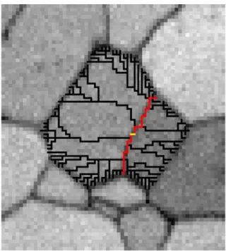
Fig. 4. Starting from the open frontier in yellow, all paths of minimum weight joining a closed boundary are browsed (in black). That of maximum average disorientation angle is the selected low angle boundary (in red). (For interpretation of the references to color in thisfigure legend, the reader is referred to the web version of this article.)
The result of a run (ω0= 3°,ω1= 0°) on the central grain ofFig. 1is
presented inFig. 4. The open frontier used as the origin is indicated in yellow. A minimum weight path joining the origin to any node of the surrounding closed boundary has been found and is displayed in black. There are as many paths as there are pixels on the perimeter of the grain. All frontiers are not contained in any one path. Instead, the paths favor frontiers of maximum disorientation angle because of the weight function. The picture would be different with w(E) = 1. Then, the paths would be on the radii of a circle centered on the origin.
For each path, the average weight is calculated. It is the total weight divided by the length of the path. From both nodes taken as origin, the path with the lowest average weight is kept as a solution. It correspond also to the boundary with the highest average disorientation angle. In
Fig. 4the two paths are plotted in red. They correspond to the detected low-angle boundary and split the grain into two sub-grains.
Other adaptations are required to take into account the specificities of EBSD data:
• The user chooses if the border of the EBSD map is treated like a closed boundary or not (in other words, if closing is possible at the border of the map or not).
• The best way to handle non-indexed pixels is to start with a grain detection using the MTEX routine[17]which has the advantage of detecting grains without cleaning. Then, all edges adjacent to non-indexed pixels are allocated a weight withω set at the angular
resolution of the EBSD map. Alternatively, another approach is to con-sider edges adjacent to non-indexed pixels like closed boundaries. The only exceptions are edges adjacent to non-indexed pixels that are to-tally included in a grain which are allocated a weight withω set at the angular resolution of the EBSD map. This allows boundary closing through non-indexed points rather than having tofind a path around them.
• If a grain contains several sub-grains, the choice of starting frontier (processing sequence) may slightly influence the results. Therefore, it is preferable to process the open frontiers in decreasing order of Fig. 5. Synthetic EBSD map designed with vertical disorientations of increasing angle and a Gaussian noise with standard deviation of 0.2°. The frontiers are colored according to their disorientation angle. The background is in gray. (For interpretation of the references to color in thisfigure legend, the reader is referred to the web version of this article.)
Fig. 6. Pixel to pixel disorientation profile along the blue line (Fig. 5) compared with the disorientation without the noise.
Table 1
Summary of the most interesting results obtained on the synthetic EBSD map ofFig. 5. ω0 (°) ω1 (°) Lowest disorientation angle boundary identified (°) Artifacts ALGrId 0.9 0.2 0.4° None Classical Grain identification 0.8 – 1.3° None Classical Grain identification 0.7 – 1.1° 8 isolated pixels GBC 1.4 ≥0.2 0.9° None GBC 1 0.7° 0.7 12 isolated pixels
disorientation angle. Once a low-angle boundary is detected, it is con-sidered equal to other closed boundaries in the next iteration. 4. Validation of the method
ALGrId was tested on a synthetic EBSD map (400 × 100 pixels) con-taining 19 regularly-spaced vertical boundaries with a disorientation angle varying from 0.1° to 1.9° with a step of 0.1°. A Gaussian orientation noise was added. Each pixel was rotated around a random axis by a
random angle. The random angles were chosen to follow a centered Gaussian distribution with a standard deviation of 0.2°. The resulting map is shown inFig. 5.
The pixel to pixel disorientation profile along the blue line inFig. 5is shown inFig. 6. In between the authentic boundaries, an average noise of 0.2° with some peaks at 0.7° was measured. In the whole map, the maximum orientation noise reached 1°. InFig. 6, thefirst boundary that is clearly distinguishable from the noise has a disorientation angle of 0.9° (situated at 180 pixels).
Fig. 7. Some results using ALGrId with different parameters to detect grains in the map ofFig. 5(Grains in random colors). (For interpretation of the references to color in thisfigure legend, the reader is referred to the web version of this article.)
ALGrId was applied to the synthetic map withω0andω1ranging
from 2° down to 0° with a step of 0.1°. The most relevant results are reported inTable 1and others are sampled inFig. 7.
Let us focusfirst on results where ω0=ω1which are equivalent to
the classical grain identification (Fig. 7). Boundaries with lower disori-entation angles are detected with decreasing values ofω0. Artifacts are
generated whenω0≤ 0.7 (8 isolated pixels are misidentified in the
case withω0=ω1= 0.7°). In this case, the lowest disorientation
angle boundary detected is 1.1°. Considerable improvement is seen using ALGrId. The best run is obtained withω0= 0.9° andω1= 0.2°
and successfully detects the 0.4° disorientation angle boundary with no artifacts. Any other set of parameters doesn't improve the resolution but creates artifacts (seeFig. 7). The results of the GBC (presented in
Table 1but not inFig. 7) are in between ALGrId and the classical grain detection.
ALGrId gives the best results withω0being slightly above the peak
disorientation angle of the orientation noise andω1set at the average
noise level. If no easy evaluation of the noise level is possible a compro-mise can be found by takingω0sufficiently high to ensure that the all
open frontiers really belong to a boundary. Then any choice ofω1in
the noise level should provide reliable results but not the best achiev-able resolution (see for example thefirst column inFig. 7).
5. Application to sub-grain detection inβ-deformed Ti-17 Titanium alloy
A Ti-17 titanium alloy wasβ-deformed by tension (ε = 32%) at a temperature of 920 °C and then helium quenched. An FEI QUANTA 600 FEG microscope equipped with an Oxford Instruments EBSD system (Nordlys F camera) was used to acquire the map shown inFig. 8(the step size was 2μm). A typical β-deformed substructure was obtained
[18,19]. Serratedβ-grain boundaries with well developed sub-grains are clearly seen on the KPQ map (Fig. 8a). The corresponding sub-grain boundaries (Fig. 8b) mostly have disorientation angles lower than 3° (only few boundary segments are delimited by 5° disorienta-tions). The classical grain reconstruction withω0= 2° fails to detect
the sub-grains and creates artifacts (Fig. 8c)
Both the GBC and ALGrId methods were applied to the central grain (with parametersω0= 3° andω1= 0.3°). The resulting grain
detec-tions are given inFig. 9.
Both methods show some improvement with respect to classical grain identification. ALGrId detected successfully the sub-grains that are visible on the KPQ image (CompareFigs. 8a and9a). On the contrary, the GBC detected only some sub-grains accurately (Fig. 9b). However, it missed some obvious boundaries and simultaneously created some artifacts. In all cases, ALGrId gave better results than GBC. Any compar-ison of both methods should also include a comparcompar-ison of simplicity and rapidity. In this respect, the GBC runs faster. Our implementation of the Dijkstra algorithm is optimized for fast running speed (use of a binary heap[16]). This allows ALGrId to run in a reasonable time.4
6. Conclusions
The classical method to identify grains fails when applied to bound-aries having disorientation angles of the same order as the relative an-gular resolution of EBSD. In this case, artifacts are generated.
A new method to detect sub-grains and/or low angle boundaries be-yond the angular resolution of EBSD is proposed. It is called ALGrId (Anti-Leak Grain Identification) and finds in an EBSD map boundaries of high average disorientation angle. This new method improves the de-tection of grains compared to the classical algorithm and to Grain Boundary Completion.
Applied to deformed titanium, it successfully identified sub-grains without creating artifacts.
Acknowledgements
The authors acknowledge Prof. F. Wagner (LEM3) for providing the T40 EBSD map as well as K. Larsen from Oxford Instruments for the description of the GBC algorithm. The authors really appreciated the implication of both reviewers whose comments and questions did not Fig. 9. Detection of sub-grains in the central grain ofFig. 8. Each sub-grain is colored randomly a) the result of ALGrId, b) the result of GBC.
4
Approximately proportional to N log(N), that is a grain detection takes usually 2– 3 min on a 106
only improve the quality of the paper but also lead to ideas for the improvement of ALGrId's algorithm.
References
[1] F. Barou, C. Maurice, J.-M. Feppon, J. Driver, Sub-grain boundary mobilities during recovery of binary Al–Mn alloys, Int. J. Mater. Res. 100 (2009) 516–521,http://dx. doi.org/10.3139/146.110057.
[2] L. Germain, N. Gey, M. Humbert, Reliability of reconstructed [beta]-orientation maps in titanium alloys, Ultramicroscopy 107 (2007) 1129–1135,http://dx.doi.org/10. 1016/j.ultramic.2007.01.012.
[3] F.J. Humphreys, Review grain and subgrain characterisation by electron backscatter diffraction, J. Mater. Sci. 36 (2001) 3833–3854,http://dx.doi.org/10.1023/A: 1017973432592.
[4] C. Maurice, R. Quey, R. Fortunier, J.H. Driver, High angular resolution EBSD and its materials applications, in: D.A. Molodov (Ed.), Microstruct. Des. Adv. Eng. Mater, Wiley-VCH Verlag GmbH & Co. KGaA, 2013, pp. 339–365.
[5] F.J. Humphreys, Y. Huang, I. Brough, C. Harris, Electron backscatter diffraction of grain and subgrain structures— resolution considerations, J. Microsc. 195 (1999) 212–216,http://dx.doi.org/10.1046/j.1365-2818.1999.00579.x.
[6] N.C. Krieger Lassen, The relative precision of crystal orientations measured from electron backscattering patterns, J. Microsc. 181 (1996) 72–81,http://dx.doi.org/ 10.1046/j.1365-2818.1996.95376.x.
[7] V. Randle, Microtexture determination and its applications, Maney for the Institute of Materials, Minerals and Mining2003.
[8] F.J. Humphreys, P.S. Bate, P.J. Hurley, Orientation averaging of electron backscattered diffraction data, J. Microsc. 201 (2001) 50–58, http://dx.doi.org/10.1046/j.1365-2818.2001.00777.x.
[9] F. Barou, (PHD Thesis) École Nationale Supérieure des Mines de Saint-Étienne, 2009.
[10] C. McMahon, B. Soe, A. Loeb, A. Vemulkar, M. Ferry, L. Bassman, Boundary identification in EBSD data with a generalization of fast multiscale clustering, Ultramicroscopy 133 (2013) 16–25,http://dx.doi.org/10.1016/j.ultramic.2013.04.009.
[11] Disclosed anonymously, Grain boundary completion, Res. Discl. (2013) (Www. researchdisclosure.com).
[12] International Organization for Standardization. ISO 13067:2011— Microbeam analysis— electron backscatter diffraction — measurement of average grain size n.d. [13] Floodfill. Wikipedia Free Encycl 2014.
[14] D.J. Prior, Problems in determining the misorientation axes, for small angular misorientations, using electron backscatter diffraction in the SEM, J. Microsc. 195 (1999) 217–225,http://dx.doi.org/10.1046/j.1365-2818.1999.00572.x.
[15] E.W. Dijkstra, A note on two problems in connexion with graphs, Numer. Math. 1 (1959) 269–271,http://dx.doi.org/10.1007/BF01386390.
[16] T.H. Cormen, C.E. Leiserson, R.L. Rivest, C. Stein, Introduction to Algorithms, 3rd ed. The MIT Press, Cambridge, Mass, 2009.
[17] F. Bachmann, R. Hielscher, H. Schaeben, Grain detection from 2d and 3d EBSD data— specification of the MTEX algorithm, Ultramicroscopy 111 (2011) 1720–1733,
http://dx.doi.org/10.1016/j.ultramic.2011.08.002.
[18] N. Allain-Bonasso, F. Wagner, S. Berbenni, D.P. Field, A study of the heterogeneity of plastic deformation in IF steel by EBSD, Mater. Sci. Eng. A 548 (2012) 56–63,http:// dx.doi.org/10.1016/j.msea.2012.03.068.
[19] D.L. Bourell, H.J. McQueen, Thermomechanical processing of iron, titanium, and zir-conium alloys in the bcc structure, J. Mater. Shap. Technol. 5 (1987) 53–73,http:// dx.doi.org/10.1007/BF02833686.