HAL Id: hal-00963802
https://hal.archives-ouvertes.fr/hal-00963802
Submitted on 22 Mar 2014HAL is a multi-disciplinary open access
archive for the deposit and dissemination of sci-entific research documents, whether they are pub-lished or not. The documents may come from teaching and research institutions in France or abroad, or from public or private research centers.
L’archive ouverte pluridisciplinaire HAL, est destinée au dépôt et à la diffusion de documents scientifiques de niveau recherche, publiés ou non, émanant des établissements d’enseignement et de recherche français ou étrangers, des laboratoires publics ou privés.
applied to rubber like materials and soft tissues
Marie Rebouah, Grégory Chagnon
To cite this version:
Marie Rebouah, Grégory Chagnon. Permanent set and stress softening constitutive equation ap-plied to rubber like materials and soft tissues. Acta Mechanica, Springer Verlag, 2014, pp.1-14. �10.1007/s00707-013-1023-y�. �hal-00963802�
(will be inserted by the editor)
M. Rebouah · G. Chagnon
Permanent set and stress softening constitutive equation
applied to rubber like materials and soft tissues
Received: date / Accepted: date
Abstract Many rubber like materials present a phenomenon known as Mullins effect. It is characterized by a difference of behavior between the first and second loadings and by a permanent set after a first loading. Moreover, this phenomenon induces anisotropy in an intially isotropic material. A new constitutive equation is proposed in this paper. It relies on the decomposition of the macromolecular network into two parts: chains related together and chains related to fillers. The first part is modeled by a simple hyperelastic constitutive equation whereas the second one is described by an evolution function introduced in the hyperelastic strain energy. It contributes to describe both the anisotropic stress softening and the permanent set. The model is finally extended to soft tissues mechanical behavior that present also stress softening but with an initially anisotropic behavior. The two models are successfully fitted and compared to experimental data.
Keywords Mullins effect · stress softening · permanent set · constitutive equation · rubber like materials · soft tissues
1 Introduction
Despite many different studies, the accurate prediction of rubber like materials mechanical behavior is still an open issue. These materials have the great capacity to endure large deformations and cyclic conditions. Nevertheless, they present also highly non-linear phenomena which make difficult to truly model them. In this paper, it is proposed to focus on three main phenomena. The first phenomenon is the stress softening [1] that occurs between the first and second loadings. This stress softening can be imputed to chain microstruc-ture rearrangements in the material [2] and depends on the maximal strain reached. Indeed, once the previous maximum strain is exceeded, the loading curve comes back on the primary curve [3–6]. The second phe-nomenon often observed for rubber like materials is the permanent set. This phephe-nomenon is characterized by a residual strain that depends on the maximal strain reached and of the composition of the material i.e. the amount of fillers [7–9]. The third phenomenon is the induced anisotropy by the stress softening. It has been observed that the stress softening of a material is maximal for a second loading along the direction of the first loading and minimum for a second loading along the orthogonal direction to the first loading direction [8, 10–14]. These three phenomena are known as the Mullins effect.
For several years, many authors developed models to predict the behavior of rubber like materials. The first models were principally isotropic [15–19]. Later some constitutive equations taking into account permanent
M. Rebouah
UJF-Grenoble 1 / CNRS / TIMC-IMAG UMR 5525, Grenoble, F-38041, France. G. Chagnon
UJF-Grenoble 1 / CNRS / TIMC-IMAG UMR 5525, Grenoble, F-38041, France. Tel.: +334 56 52 00 86
Fax: +334 56 52 00 44
set were developed. Dorfmann and Ogden [20] proposed a model by means of the pseudo-elasticity, which is an isotropic model able to take into account the stress softening and the permanent set. This model is one of the most employed and was implemented into a Finite Element code. The eight-chain model [21] , with its analytical form easily usable than other chain models, stimulates the development of micro-physically motivated models. The micro spherical models first proposed by [22–24] and then by [8, 11, 25, 26] are con-stitutive equations that allow to describe hyperelasticity, viscoelasticity and plasticity. But it also permits to describe the induced anisotropy by stress softening by means of this repartition of directions in space. The space repartition pemits to use different evolution functions or identical evolution functions that would evolve differently. It is to note that according to the spatial discretisation used some unphysical anisotropy can be induced by the model used [27, 28]. But few models are able to take into account stress softening, permanent set and induced anisotropy of a material. Recently, Rickaby and Scott [29] developed a constitutive equations to describe stress softening, permanent set and relaxation behavior but limited to equibiaxial loading. Itskov et al.[30] also proposed recently a model to take into account anisotropic softening and permanent set by means of a pseudo strain energy. Moreover, Merckel et al.[8, 31] developed a tridimensional model describing the permanent set and the stress softening, but considered then as independent phenomena.
In the last few years, it was observed that the understanding of the behavior of soft tissues get improved [32–35] and thus the multiplication of model appears. It is well known that soft tissues present a similar be-havior to rubber like materials. Thus, soft tissues present also a stress-softening. It was observed for example, for arteries [36, 37], venas [38], vaginal tissues [39], oesophageal [40] ... Inspired by the rubber like mate-rials phenomenological models [20], several authors proposed pseudo elastic models adapted to soft tissues [41, 42]. Phenomenological models based on 3D generalization model were also proposed, Alastrue et al, [43] readapted exponentiel model and the 8 chains model. Nevertheless, soft tissues present also an initial anisotropic behavior due to their structure. Most of the soft tissues are composed of a matrix reinforced by fibers, thus the models built for them are based on initially anisotropic constitutive equation that depends on the orientation of the fibers [40, 44–48]. Some models were adapted to take into account the stress softening and the permanent set [37, 49]. Generally the stress softening is treated by considering that it only occurs in the fibres and not in the matrix.
Most of the existing models do not treat simultaneously the three phenomena of the Mullins effect. A new constitutive equation is developed here by means of a micro spherical model, to take into account the stress softening with the permanent set and the induced anisotropy for rubber like materials by using a formulation with strain invariant and by considering this phenomena as independant. This model is then adapted to soft tissues by adding an initial anisotropy with fibers. In this way, in Section 2 an experimental study lead on a filled silicone rubber is presented highlighting the stress softening, the induced anisotropy and the permanent set. In Section 3, constitutive equations are developed to take into account these effects for rubber like ma-terials. Section 4 presents a successful comparison of the model with the experimental data. Finally, Section 5 presents the extension of the constitutive equation to soft tissues, the results are compared to experimental data from literature.
2 Experimental data on silicone rubber 2.1 Materials
Two materials are used for this study, an initially isotropic one, a silicone rubber and an initially anisotropic one, an ovine vena cava [50]. The silicone rubber used is a Heat Cured Silicone (HCS) also called Hot Tem-perature Vulcanization (HTV) which contains 30% of fillers (silica). This filled silicone rubber is vulcanized with a peroxyde starter. A plate of 185 mm length, 170 mm width and 2.5 mm thick is molded and vulcanized
under an increasing pressure (0.1MPa to 0.5 MPa) and a temperature 180◦C. No experimental study is lead
on the soft tissues. The experimental data are used from Pe˜na et Doblar´e [50].
2.2 Classical tensile tests
Tensile tests were realized on samples of 15 mm length, 2.5 mm width and 2.5 mm thick cut from the molded
rectangular plate. First, the influence of the strain rate is evaluated. Cyclic tensile tests up to λ = 2.5 (λ
s−1, 0.167 s−1, 1. s−1, 1.667 s−1. For these small variations of the strain rate, there is no significant influence on the mechanical behavior of rubber like material. For the study it is thus chosen to perform all the following
tests at a strain rate of 1.s−1. Second, silicone specimens were submitted to cyclic loading up to a fixed stretch.
1.0 1.5 2.0 2.5 0 2 4 6 8 C a u ch y st r e ss ( M P a )
Fig. 1 Cyclic tensile test on HTV silicone at a strain rate of 1s−1
Each of the specimens was subjected to two loading unloading cycles up toλ = 2. After completion of the
second unloading cycle, each specimen was then loaded up to a stretch ofλ = 2.5. No recovery time was
allowed during the two loading unloading cycles. The results of one test can be observed in Fig.1. The stress softening and the permanent set can be observed as an hysteretic behavior, which is not taken into account in this study.
2.3 Induced anisotropy by the Mullins effect
In this section, it is proposed to highlight the induced anisotropy by the Mullins effect in the HTV silicone rubber. First, a large sample of silicone is prepared for a pure shear test, it is presented in Fig.2(a). This sample
of 40 mm length, 15 mm width and 2 mm thick is submitted to a cyclic tensile test up toλ = 2. This test is
performed at a strain rate of 1 s−1. Next, several samples are cut from this sample along different orientations
(α = 0◦
,α = 25◦
,α = 45◦
,α = 90◦
) compared to the first tensile direction as illustrated in Fig.2(b). Four new samples of 15 mm length, 2.5 mm width and 2 mm thick are obtained. Each specimen is subjected to a
loading unloading cycle up toλ = 2.5 at a strain rate of 1 s−1.
The mechanical test realized and described in Fig.2 can be studied in different configurations (cf. Fig.2(c)).
The first configuration C0 is the initial configuration of the sample (before pure shear test). The C1
config-uration is the intermediary configconfig-uration (after pure shear test) and C2is the final configuration where the
four samples cut according to different orientations from the pure shear test sample are submitted to a tensile test. By means of these tests, several observations can be done. First, the influence of the orientation of the
samples is highlighted in Fig.3(a). For this representation, it is considered that the initial configuration is C1
and not C0(cf. Fig.2(c)). The reference configuration is thus considered after the pure shear test, that means
that the stress softening is studied without initial permanent set induced by the pure shear test. This allows to
focus on the influence of the orientation. It is observed that for an orientation ofα = 90◦
the material has the
same behavior as a first loading (i.e. behavior similar to a virgin material). For an orientation ofα = 0◦
the mechanical behavior is a classical second loading without change of direction. The intermediary orientations
α = 25◦
andα = 45◦
present a behavior between a first and second loadings, the stress softening is more
important for the orientation ofα = 25◦
than for the orientation of α = 45◦
but the two curves come back on the same point on the first loading curve. These conclusions are the same as previously shown on a RTV
(a) (b) C 0 C 1 C 2 (c)
Pure Shear Uniaxial tension
Direction of the first loading
Fig. 2 Experimental device used to highlight induced anisotropy by Mullins effect (a) pure shear test, (b) geometry of the cut specimens inside the pure shear specimen, (c) definition of the configurations, (C0) initial configuration, (C1) configuration after
the pure shear test, (C2) configuration after the pure shear and tensile tests.
1.0 1.5 2.0 2.5 0 2 4 6 8 10 1.0 1.5 2.0 2.5 0 2 4 6 8 10 a C a u c h y s t r e s s ( M P a ) 0° 25° 45° 90° b C a u c h y s t r e s s ( M P ) 0° 25° 45° 90°
Fig. 3 Influence of the angle between the first and second loadings on the stress softening compared to (a) configuration C1, i.e.
without taking into account the permanent set after the first loading and (b) compared to configuration C0, i.e. by taking into
account the permanent set after the first loading
silicone [51].
It is also proposed to represent these four tensile tests by taking into account the complete history of the
ma-terial i.e. compared to the initial configuration C0(cf. Fig.2(c)), i.e. the permanent set generated by the pure
shear test is now taken into account. The results are presented in Fig.3(b). The same stress softening as in Fig.3(a) is observed, and also the amount of permanent set endured lasting the pure shear test for the different samples. It is observed that more the orientation is close to the first loading direction more the permanent set
is important. Indeed, for an orientation ofα = 0◦
it can be observed an initial permanent set (due to the pure
shear test) ofλresid= 1.136 and at the opposite for the sample cut at α = 90◦the initial permanent set is null.
3 Constitutive equation 3.1 General form
Recently, Rebouah et al [26] developed a constitutive equation written with strain invariants to predict the anisotropic stress softening in filled silicone rubbers but without permanent set. Based on the idea of
Govin-djee [53], the strain energy density of the material Wsiliconeis additively decomposed into two parts: one that
represents the strain energy of the chains linked to filler Wc fand an other part that represents the strain energy
of the chains linked to other chains Wcc. The total strain energy density is thus Wsilicone= Wcc+ Wc f. Rebouah
et al [26] considered that only Wc f can evolve with the Mullins effect. In our approach, it is also proposed to
describe the permanent set by means of Wc f. Thus Wc fis represented by an anisotropic strain energy function
that can record the deformation history of the material. Any micro-sphere model defined by a spatial direction
repartition A(i)can be chosen. The dilatation in each direction is defined by means of I4(i)= A(i).CA(i)where
C is the right Cauchy-Green deformation tensor, defined by C= FTF, and F is the deformation gradient. The
general form of the model is:
Wsilicone= Wcc(I1,I2) +
n
∑
i=1
ω(i)F(i)W(i)
c f (I (i)
4 ). (1)
Wccis an hyperelastic energy density, I1, I2are the first and second strain invariants of C. W(i)
c f is the
hypere-lastic strain energy associated with each direction andω(i)represents the weight of each direction. They are
given by Bazant and Oh[54], F(i)is the Mullins effect evolution function. The HTV silicone does not present
strain hardening, thus it is decided to use a strain energy that is not presenting a large increase of slope with
deformation. The Mooney [15] strain energy function is chosen for Wccand a particular form is proposed for
Wc f. Previously ([26]) the quadratic equation proposed by Kaliske et al, [52] was used. Nevertheless for this
material this equation presents a stress hardening too important to represent the considered material, thus a function with a few hardening is used:
if I4(i)≥ 1 Wc f(i)(I4(i)) =K2
∫ v u u t I4(i)− 1 I4(i) dI4(i) else 0 (2)
where K is the only material parameter. It is to note that it is considered here that the strain energy in each direction is considered only in tension.
Rebouah et al[26] proposed an evolution function which depends on the first and fourth invariants with only
one material parameterη. The evolution function is the product of three terms. The first is an isotropic term
which depends only on the first invariant and represents the global deformation of the material (similar to isotropic approaches), the second represents the maximal deformation of each direction of the material and the third the triaxiality of the loading state. In this paper, it is proposed to adapt the constitutive equation to represent both stress softening and permanent set. For the HTV silicone rubber, the isotropic part is useless, then it is omitted here. The evolution of the stress softening is then different for this material the powers of the two terms of the evolution function are changed and can be considered as parameters. The proposed function is:
F(i)= 1 − η
(
I4 max(i) − I4(i) I4 max(i) − 1 )β( I4 max(i) I4 max )γ (3) As proposed in literature [55], the stress-softening is described by the difference between the current strain and the maximum strain. The first term of the equation is the ratio of this difference between the current and undeformed states. The second term represents the triaxiality of the strain by the ratio of the strain in one direction compared to the maximum one. The powers assigned to each term must be chosen to represent at the best the mechanical behavior of the material and to avoid numerical problems. It is to note that these functions are phenomenological and their form is not motivated by micro mechanical observations.
The parameters η, β and γ influence simultaneously the stress softening and the permanent set of the
material. I4max(i) represents the maximal value of I4(i) for the whole material history for each direction and
permanent set a strong restriction proposed by Rebouah et al [26] is suppressed here, the evolution function
F(i)is allowed to become negative. That means that the zero stress of a direction is no longer reach for zero
deformation but for a deformation depending on the parameterη. It is to note that the evolution function F(i)
depends on two different maximal values of the fourth invariant, i.e in the considered direction, and for the whole material. Finally the Cauchy stress is obtained by:
σsilicone= σcc+ σc f− pI (4)
Whereσccis the part of the Cauchy stress that represents the chains linked to other chains andσc f the part
of the Cauchy stress that represents the chains linked to fillers, expressed as:
σcc= 2B ∂Wcc ∂ I1 + 2(I1B − B2) ∂ Wcc ∂ I2 (5) σc f = 2 42
∑
i=1 ω(i)F(i)∂Wc f ∂ I4(i) (i) FA(i)⊗ A(i)FT (6)where the 42 directions repartition proposed by Bazant and Oh [54] were chosen, in this study.
3.2 Validity of the model
It remains to verify that the presented model is in agreement with the requirements of thermodynamics (see e.g. Coleman and Gurtin [56]). If only isothermal processes is considered, the Clausius-Duhem inequality must be satisfied −∂ Wsilicone ∂ I4 max(i) ˙ I4 max(i) ≥ 0 (7) −∂ Wsilicone ∂ I4 max ˙ I4 max≥ 0 (8)
where ˙I4 max(i) ≥ 0 and ˙I4 max≥ 0 are the maximum deformation increase rates. By means of manipulations of
Eqs. (7), (8) and (1), it can be easily established the next sufficient relations with the functions F(i):
∂ F(i)
∂ I4 max(i) ≤ 0 ∀i (9)
∂ F(i)
∂ I4 max
≤ 0 ∀i (10)
Considering, the generic form of the evolution constitutive equation (3), it can be explicitely written that:
∂ F(i)
∂ I4 max(i) = −ηα (
I4 max(i) −1)−(I4 max(i) −I(i)4 ) (
I4 max(i) −1)2
(
I(i)4 max−I4(i) I4 max(i) −1 )β −1( I4 max(i) I4 max )γ −ηβ 1 I4 max (
I4 max(i) −I4(i) I4 max(i) −1 )β( I4 max(i) I4 max )γ−1 (11) ∂ F(i) ∂ I4 max = −ηβ I4 max(i) (
I4 max(i) − I4(i) I4 max(i) − 1 )β( I4 max(i) I4 max )γ−1 (12)
To verify Eqs (9) and (10), the conditions to verify areα > 0, β > 0 and(I4 max(i) − 1)−(I4 max(i) − I4(i))>0.
This last condition is automatically verified if I4(i)≥ 1. It is verified for I4(i)≤ 1 by means of Eq (1) as no
4 Simulations of the model
To validate the model, it is proposed to compare its simulations to the different mechanical tests. The values
of the material parameters were fitted on the different mechanical tests. The obtained values are: C1= 0.3
MPa, C2= 0.15 MPa, K = 1.6 MPa, η = 5, β = 0.5 and γ = 2.5.
4.1 HTV on a tensile test
First the cyclic tensile test presented in Fig.1 is compared to the prediction of the model. The results obtained are illustrated in Fig.4. These results are satisfactory since it can be observed that the Mullins effect and the permanent set are quite well described by the model.
1.0 1.5 2.0 2.5 0 2 4 6 8 C a u ch y st r e ss ( M P a )
Fig. 4 Comparison of the prediction of the model (full lines) to experimental data (dotted lines)
4.2 HTV on a tensile test after a pure shear test
In this section, it is proposed to compare the model to the experimental results of the pure shear test followed by tensile tests according to different orientations. A comparison between the model and the tests is proposed in Fig.5. It is to note that the first and second loadings (and thus the elongation) do not correspond to the
same test. For each test the definition ofλ corresponds to the elongation in the tensile test direction whatever
the experiment. Every simulated orientations present a similar behavior to the experimental results, thus the same observation as the one made in paragraph 2.3 can be done. Furthermore it is shown that the model is
able to take well into account the induced anisotropy. Finally for the curve atα = 25◦
it is observed that the
second loading curve of the model present a rupture of slope aboutλ = 1.8. This phenomenon is due to the
discretization along the 42 directions of Bazant and Oh (1986). The problem is that the discretization in 42 directions creates a numerical anisotropy, as explained in literature [27]. This phenomenon can be avoided with a full integration in space, nevertheless the computational formulation become more complicated and it becomes very time consuming. Despite discretization problems, these results proved the ability of the model to take into account the induced anisotropy and the permanent set.
1.0 1.5 2.0 2.5 0 3 6 9 1.0 1.5 2.0 2.5 0 3 6 9 1.0 1.5 2.0 2.5 0 3 6 9 1.0 1.5 2.0 2.5 0 3 6 9 C a u c h y s t r e s s ( M P a ) 2C exp 1C m odel 2C m odel C a u c h y s t r e s s ( M P a ) 2C exp 1C m odel 2C m odel C a u c h y s t r e s s ( M P a ) 2C exp 1C m odel 2C m odel C a u c h y s t r e s s ( M P a ) 2C exp 1C m odel 2C m odel
Fig. 5 Comparison with experimental oriented data and the model. The black full lines represent the theoretical first loading in uniaxial tension (1Cmodel), the black dotted lines represent the second loadings (i.e. the tensile test) for the different orientations (2Cmodel). The red dashed lines represent the experimental results for the different oriented samples of tensile tests after the pure shear test (2Cexp)
4.3 Analysis of the model simulations
In this part, it is proposed to analyze the evolution of the stress softening along the 42 spatial directions. The
principal request directions during a cycling tensile test are observed along the direction of tension→x , where
the maximal deformations are reached for different cycles until a maximal elongation ofλ = 1.5, then λ = 2.
andλ = 2.5. The 42 directions are represented in projection in the plan (→z ,→y ) in Fig.6 as [22]. It is to note
that many directions have the same angle with the→x direction. They are summarized by the definition of 4
circles.
The stressσxxwhich corresponds to the stress in the tensile direction. It is by construction the tensorial sum
of stresses along the 42 directions [54]. More a direction is closer from direction→x , more its contribution
toσxxis important. All the directions that belong to a same circle provide the same contribution in the case
of uniaxial tension in direction→x . Thus, for clarity of the figure only one direction per circle is presented.
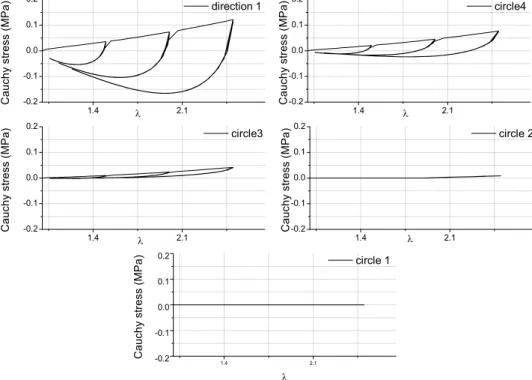
The stress strain behavior of each direction is presented in Fig.7. It appears that the most loaded direction is
direction 1, which is consistent since it corresponds to the tensile direction→x . Nevertheless it is observed that
the directions which belong to the circle 3 (4-5-6-7) and to the circle 4 (18-19-20-21) endure also an important deformation and generate important stresses. It can also be observed that the directions which belong to the circle 2 (10-11-12-13-14-15-16-17) have very few influence, and the directions which belong to the circle 1 (2-3-8-9) are equal to zero as they are loaded only in compression. Besides direction 1, circles 3 and 4 present a negative part of the Cauchy stress during second loadings, that means that these directions present a permanent set. The directions that belong to circle 1 and 2 are still superior or equal to zero thus they do not
present permanent set.
The evolution function generates a new equilibrium position, meaning that the zero stress state is no longer reached for zero deformation. This new equilibrium depends on the maximum deformation and is thus more
important for directions close to direction→x . This is illustrated by Fig.8. It is observed that along the direction
1, the circle 3 and 4 the evolution function becomes negative, thas means that the material presents a zero stress, and thus a permanent set. It is to note that the directions where the evolution function become negative are the same direction for which the stress become negative and thus directions which generate permanent set. For this study the 42 directions proposed by Bazant and Oh (1986) were used, nevertheless the other directions repartition proposed by the same author can also be used. It was proved that the results observed are identical but they are not presented in the paper.
1 2 3 4 5 6 8 9 10 11 12 13 14 15 16 17 18 7 19 21 20 x z y Circle 1 Circle 2 Circle 3 Circle 4
Fig. 6 Representation of the 42 Bazant and Oh directions in the plan(→z ,→y )
5 Adaptation of the constitutive equation to soft tissues 5.1 Adaptation of the model
It is proposed here to adapt the general form of the model previously described to non initially isotropic materials, i.e. soft tissues. This anisotropy is imputed to the presence of fibers, often collagen [35], into the matrix of the tissue. In many soft tissues, there exist two main fibers orientations (the model will be developed for 2 directions, but the proposed principle would be the same for more directions). The orientation of these fibers depends on the studied soft tissues [40, 57–60]. As classically done in literature, it is proposed to model the soft tissues mechanical behavior as the sum of three terms. The first part represents the behavior of the matrix, the second and third parts represent respectively the mechanical behavior of the fibers oriented in the two directions.
Wsoft-tissue= Wmatrix+ Wfiber1+ Wfiber2 (13) It is also often assumed that the fibers can only endured tension, i.e. that no stress is generated in compression. The principle is to propose a strain energy that can simulate the stress softening both in the matrix and in the
1.4 2.1 -0.2 -0.1 0.0 0.1 0.2 1.4 2.1 -0.2 -0.1 0.0 0.1 0.2 1.4 2.1 -0.2 -0.1 0.0 0.1 0.2 1.4 2.1 -0.2 -0.1 0.0 0.1 0.2 1.4 2.1 -0.2 -0.1 0.0 0.1 0.2 C a u c h y s t r e s s ( M P a ) di recti on 1 C a u c h y s t r e s s ( M P a ) ci rcl e4 C a u c h y s t r e s s ( M P a ) ci rcl e3 C a u c h y s t r e s s ( M P a ) ci rcl e 2 C a u c h y s t r e s s ( M P a ) ci rcl e 1
Fig. 7 Representation of the first component of the stress tensor (σxx) for cyclic tensile test up toλ = 2.5
fibers. In the matrix, an initially isotropic strain energy is considered, which is similar to the one proposed for silicone rubbers in part 3. The same form is thus proposed
Wmatrix= Wcc(I1) +
n
∑
i=1
ω(i)F(i)W(i)
c f (I (i)
4 ). (14)
Different hyperelastic strain energies are used, as soft tissues present more strain hardening than silicone
rubber. Classical strain energies are chosen for Wcc(I1) [61, 62] and Wc f(i)[52], they are defined as:
Wcc(I1) = C1exp(C2(I1− 3)2− 1) (15) W(i) c f = K(I (i) 4 − 1) 2 (16)
where C1, C2and K are material parameters. The evolution function F(i)of the matrix is the same as the one
used for silicone rubber model, described in Eq.(3).
The strain energy for fiber j is the product of an hyperelastic strain energy Wcf-fiberjand an evolution function
F
fiber( j) to describe the Mullins effect:
Wfiber1= F
fiber( j).Wcf-fiberj (17)
The hyperelastic strain energy of each fiber is noted Wcf-fiberj[63] is expressed as:
Wcf-fiber j= Kf 2 exp(I ( j) 4 − I ( j) 40) 2 (18)
1.4 2.1 -4 -2 0 1.4 2.1 -4 -2 0 1.4 2.1 -4 -2 0 1.4 2.1 -4 -2 0 1.4 2.1 -4 -2 0 E v o l u t i o n F u n c t i o n di recti on 1 E v o l u t i o n F u n c t i o n ci rcl e4 E v o l u t i o n F u n c t i o n ci rcl e3 E v o l u t i o n F u n c t i o n ci rcl e 2 E v o l u t i o n F u n c t i o n ci rcl e 1
Fig. 8 Representation of the evolution function for cyclic tensile test up toλ = 2.5
Kf is a material parameter and I4( j)0 matches to the value of I4( j)for which the stress hardening of the material
appears. Finally, due to the hypothesis of tension in the fiber, the evolution function is also adapted for the
fibers, where only I4( j)is necessary. A simplified form of the evolution function is used compared to the one
used in Eq.(3). Indeed for the fiber only one direction is considered, that means that the third term that took into account the triaxiality is not necessary. Only the second term is consistent.
F( j) fiber= 1 − ηf ( I4 max( j) − I4( j) I4 max( j) − 1 )β (19)
Whereηf andβ are the material parameters which allows to take into account the stress softening and the
permanent set of the fibers. It is to note that in this part, it is considered that the material cannot endured compression, thus the stress cannot become negative in any direction. Nevertheless it generates the begining of the permanent set for the material. This difference compared to the last model (for rubber like materials) is due to the stress hardening of soft tissues which is very important, and thus the evolution function must be adapted to correctly describe the phenomena.
5.2 Comparison with experimental data
To highlight the ability of the model to mimic soft tissues, it is proposed to compare it by means of the experimental data of Pe˜na and Doblar´e [50] considering first and second loadings at different maximum
deformation in ovine vena cava during uniaxial tension. The orientation of the fibers was chosen atα = 45◦
.
1.0 1.2 1.4 1.6 1.8 0.0 0.3 0.6 model 135° exp 135° C a u ch y st r e ss ( M P a ) model 45° exp 45°
Fig. 9 Experimental data and comparison with the model for oriented sample of 45◦and 135◦in the tissue
0.16MPa; K= 0.13MPa; Kf= 0.5MPa; η = 2., ηf = 5 and β = 2. As observed in Fig.9 the experimental data
obtained for loading reloading cycles at different stretches are well described by the model. Fig.9(a) represents
the theorical tensile test for a tensile test along the axial direction for a value ofα = 45◦
and Fig.9(b) along the circumferential direction. For both tests it is observed that the hyperelastic behavior, the stress softening, the permanent set and the initial anisotropy are well taken into account. In this case the induced anisotropy is not visible on the experimental data, nevertheless the model can also take it into account.
6 Conclusion
As explained and shown in the present paper a simple model is proposed here to take into account several effects of the Mullins effect. This model is adapted for both rubber like materials and soft tissues. Compared to literature [8, 13] the major difference is that the permanent set and the stress softening are considered as correlated phenomena and thus the material parameters allow to represent simultaneously the stress softening and the permanent set. Due to the use of two different materials (HTV and soft tissues) different expressions were used for the strain energies and the evolution functions. Nevertheless the discretization by a micro sphere model represents well the both material. Finally, by means of the extension of the model to soft tissues, the initially anisotropy of the materials can be taken into account independently of the induced anisotropy due to the stress softening. For both of these materials the constitutive equations were successfully compared to experimental data to take into account simultaneously the stress softening of the material, the permanent set, the induced anisotropy or the initial anisotropy of the material. Furthermore, due to the formulation in strain invariant of the constitutive equations, can easily be implemented into a Finite Element code.
Acknowledgements The authors thank Professor Estefania Pe˜na for helpful information on the experimental data of Pe˜na and Doblar´e [50].
References
1. Mullins, L. (1948). Effect of stretching on the properties of rubber. Rubb. Chem. Technol., 21, 281–300. 2. Mullins, L. (1969). Softening of rubber by deformation. Rubber Chem. Technol., 42, 339–362.
3. Gurtin, M. E. and Francis, E. C. (1981). Simple rate-independent model for damage. J. Spacecraft, 18(3), 285–286. 4. Simo, J. C. (1987). On a fully three-dimensional finite-strain viscoelastic damage model: formulation and computational
aspects. Comp. Meth. Appl. Mech. Engng, 60, 153–173.
5. Miehe, C. (1995). Discontinuous and continuous damage evolution in Ogden type large strain elastic materials. Eur. J. Mech., A/Solids, 14(5), 697–720.
6. Ogden, R. W. and Roxburgh, D. G. (1999). An energy based model of the Mullins effect. In Dorfmann & Muhr, editor, Constitutive Models for Rubber I. A. A. Balkema.
7. Ogden, R. W. (2004). Mechanics of rubberlike solids. In XXI ICTAM, Warsaw, Poland.
8. Diani, J., Brieu, M., and Vacherand, J. M. (2006). A damage directional constitutive model for the Mullins effect with permanentset and induced anisotropy. Eur. J. Mech. A/Solids, 25, 483–496.
9. Merckel, Y., Diani, J., Roux, S., and Brieu, M. (2011). A simple framework for full-network hyperelasticity and anisotropic damage. Journal of the Mechanics and Physics of Solids, 59(1), 75 – 88.
10. Laraba-Abbes, F., Ienny, P., and Piques, R. (2003). A new Taylor-made methodology for the mechanical behaviour analysis of rubber like materials: II. Application of the hyperelastic behaviour characterization of a carbon-black filled natural rubber vulcanizate. Polymer, 44, 821–840.
11. Itskov, M., Haberstroh, E., Ehret, A. E., and Vohringer, M. C. (2006). Experimental observation of the deformation induced anisotropy of the Mullins effect in rubber. KGK-Kautschuk Gummi Kunststoffe, 59(3), 93–96.
12. Machado, G., Favier, D., and Chagnon, G. (2012). Determination of membrane stress-strain full fields of bulge tests from SDIC measurements. Theory, validation and experimental results on a silicone elastomer. Exp. Mech., 52, 865–880. 13. Merckel, Y., Brieu, M., Diani, J., and Caillard, J. (2012). A Mullins softening criterion for general loading conditions. J.
Mech. Phys. Solids, 60(7), 1257 – 1264.
14. Dorfmann, A. and Pancheri, F. (2012). A constitutive model for the Mullins effect with changes in material symmetry. Int. J. Nonlinear Mech, 47(8), 874 – 887.
15. Mooney, M. (1940). A theory of large elastic deformation. J. Appl. Phys., 11, 582–592.
16. Treloar, L. R. G. (1943). The elasticity of a network of long chain molecules (I and II). Trans. Faraday Soc., 39, 36–64 ; 241–246.
17. Ogden, R. W. (1972). Large deformation isotropic elasticity - on the correlation of theory and experiment for incompressible rubber like solids. Proc. R. Soc. Lond. A, 326, 565–584.
18. Haines, D. W. and Wilson, D. W. (1979). Strain energy density function for rubber like materials. J. Mech. Phys. Solids, 27, 345–360.
19. Gent, A. N. (1996). A new constitutive relation for rubber. Rubber Chem. Technol., 69, 59–61.
20. Dorfmann, A. and Ogden, R. W. (2004). A constitutive model for the Mullins effect with permanent set in particule-reinforced rubber. Int. J. Solids Struct., 41, 1855–1878.
21. Arruda, E. M. and Boyce, M. C. (1993). A three dimensional constitutive model for the large stretch behavior of rubber elastic materials. J. Mech. Phys. Solids, 41(2), 389–412.
22. Miehe, C., G¨oktepe, S., and Lulei, F. (2004). A micro-macro approach to rubber-like materials - part I: the non-affine micro-sphere model of rubber elasticity. J. Mech. Phys. Solids, 52, 2617–2660.
23. Miehe, C. and G¨oktepe, S. (2005). A micro-macro approach to rubber-like materials. part II: The micro-sphere model of finite rubber viscoelasticity. J. Mech. Phys. Solids, 53, 2231–2258.
24. G¨oktepe, S. and Miehe, C. (2005). A micro-macro approach to rubber-like materials. part III: The micro-sphere model of anisotropic mullins-type damage. J. Mech. Phys. Solids, 53, 2259–2283.
25. Shariff, M. H. B. M. (2006). An anisotropic model of the Mullins effect. J. Eng. Math., 56, 415–435.
26. Rebouah, M., Machado, G., Chagnon, G., and Favier, D. (2013). Anisotropic Mullins stress softening of a deformed silicone holey plate. Mech. Res. Commun., 49(0), 36 – 43.
27. Gillibert, J., Brieu, M., and Diani, J. (2010). Anisotropy of direction-based constitutive models for rubber-like materials. Int. J. Solids Struct., 47(5), 640 – 646.
28. Ehret, A. E., Itskov, M., and Schmid, H. (2010). Numerical integration on the sphere and its effect on the material symmetry of constitutive equations- a comparative study. Int. J. Numer. Meth. Eng., 81(2), 189–206.
29. Rickaby, S. and Scott, N. (2013). A cyclic stress softening model for the Mullins effect. IJSS, 50(1), 111 – 120.
30. Itskov, M., Ehret, A., Kazakeviciute-Makovska, R., and Weinhold, G. (2010). A thermodynamically consistent phenomeno-logical model of the anisotropic Mullins effect. ZAMM - J. Appl. Math. Mech., 90, 370–386.
31. Merckel, Y., Diani, J., Brieu, M., and Caillard, J. (2013). Constitutive modeling of the anisotropic behavior of Mullins softened filled rubbers. Mech. Mater., 57(0), 30 – 41.
32. Lanir, Y. (1979). A structural theory for the homogeneous biaxial stress-strain relationshipin flat collagenous tissues. J. Biomech., 12, 423–436.
33. Lanir, Y. (1983). Constitutive equations for fibous connective tissues. J. Biomech., 16, 1–12.
34. Fung, Y. C. (1993). Biomechanics, Mechanical properties of living tissues. Springer, New York, 2nd edition edition. 35. Holzapfel, G. A. (2000). Nonlinear solid mechanics - A continuum approach for engineering. John Wiley and Sons, LTD. 36. Vande Geest, J. P., Sacks, M. S., and Vorp, D. A. (2006). The effects of aneurysm on the biaxial mechanical behavior of
human abdominal aorta. J. Biomech., 39, 1324–1334.
37. Maher, E., Creane, A., Lally, C., and Kelly, D. J. (2012). An anisotropic inelastic constitutive model to describe stress softening and permanent deformation in arterial tissue. J. Mech. Behav. Biomed. Mater., 12(0), 9 – 19.
38. Alastru´e, Pe˜na, E., Martinez, M. A., and Doblar´e, M. (2008). Experimental study and constitutive modelling of the passive mechanical properties of the ovine infrarenal vena cava tissue. J. Biomech., 41, 3038–3045.
39. Pe˜na, E., Calvo, B., Martinez, M. A., Martins, P., Mascarenhas, T., Jorge, R. M. N., Ferreira, A., and Doblar´e, M. (2010). Experimental study and constitutive modeling of the viscoelastic mechanical properties of the human prolapsed vaginal tissue. Biomech. Model. Mechanobiol., 9, 35–44.
40. Natali, A. N., Carniel, E. L., and Gregersen, H. (2009). Biomechanical behaviour of oesophageal tissues: Material and structural configuration, experimental data and constitutive analysis. Med. Eng. & Phys., 31, 1056–1062.
41. Franceschini, G., Bigoni, D., Regitnig, P., and Holzapfel, G. A. (2006). Brain tissue deforms similarly to filled elastomers and follows consolidation theory. J. Mech. Phys. Solids, 54, 2592–2620.
42. Horgan, C. O. and Saccomandi, G. (2005). A new constitutive theory for fiber-reinforced incompressible nonlinearly elastic solids. J. Mech. Phys. Solids, 53, 1985–2015.
43. Alastru´e, V., Martinez, M. A., Doblar´e, M., and Menzel, A. (2009). Anisotropic microsphere-based finite elasticity applied to blood vessel modelling. J. Mech. Phys. Solids, 57, 178–203.
44. Balzani, D., Neff, P., Schroder, J., and Holzapfel, G. A. (2006). A polyconvex framework for soft biological tissues. adjustement to experimental data. Int. J. Solids Struct., 43, 6052–6070.
45. Nerurkar, N. L., Mauck, R. L., and Elliott, D. M. (2011). Modeling interlamellar interactions in angle-ply biologic laminates for annulus fibrosus tissue engineering. Biomech Model Mechanobiol, 10, 973–984.
46. Calvo, B., Pe˜na, E., Martinez, M. A., and Doblar´e, M. (2007). An uncoupled directional damage model for fibred biological soft tissues. formulation and computational aspects. International Journal for Numerical Methods in Engineering, 69(10), 2036–2057.
47. Caner, F. C. and Carol, I. (2006). Microplane constitutive model and computational framework for blood vessel tissue. Journal of Biomechanical Engineering, 128, 419–427.
48. Driessen, N. J. B., B. C. V. C. and Baaiens, F. T.ens, F. P. T. (2005). A structural constitutive model for collagenous cardiovascular tissues incorporating the angular fiber distribution. Journal of Biomechanical Engineering, 127, 494–503. 49. Pe˜na, E., Martins, P., Mascarenhasd, T., Natal Jorge, R. M., Ferreirae, A., Doblar´e, M., and Calvo, B. (2011). Mechanical
characterization of the softening behavior of human vaginal tissue. J. Mech. Beh. Biomed. Mater., 4, 275–283.
50. Pe˜na, E. and Doblar´e, M. (2009). An anisotropic pseudo-elastic approach for modelling Mullins effect in fibrous biological materials. Mech. Res. Comm., 36, 784790.
51. Machado, G., Chagnon, G., and Favier, D. (2012b). Induced anisotropy by the Mullins effect in filled silicone rubber. Mechanics of Materials, 50, 70 – 80.
52. Kaliske, M. (2000). A formulation of elasticity and viscoelasticity for fibre reinforced material at small and finite strains. Comput. Methods Appl. Mech. Engrg, 185, 225-243.
53. Govindjee, S. and Simo, J. C. (1992). Mullins’ effect and the strain amplitude dependence of the storage modulus. Int. J. Solids. Structures, 29(14-15), 1737–1751.
54. Bazant, Z. P. and Oh, B. H. (1986). Efficient numerical integration on the surface of a sphere. Z. Angew. Math. Mech., 66, 37–49.
55. Zu˜niga, A. E. and Beatty, M. F. (2002). A new phenomenological model for stress-softening in elastomers. Z. Angew. Math. Mech., 53, 794–814.
56. Coleman, B. D. and Gurtin, M. E. (1967). Thermodynamics with internal state variables. J. Chem. Phys., 47, 597–613. 57. Schr¨oder, J., Neff, P., and Balzani, D. (2005). A variational approach for materially stable anisotropic hyperelasticity. Int.
J. Solids. Struct., 42, 4352–4371.
58. Li, D. and Robertson, A. M. (2009). A structural multi-mechanism constitutive equation for cerebral arterial tissue. Int. J. Solids S., 46(1415), 2920 – 2928.
59. Ehret, A. E. and Itskov, M. (2009). Modeling of anisotropic softening phenomena: Application to soft biological tissues. Int. J. Plast., 25, 901919.
60. Pe˜na, E. (2011). Prediction of the softening and damage effects with permanent set in fibrous biological materials. J. Mech. Phys. Solids, 59, 1808–1822.
61. Demiray, H. (1972). A note on the elasticity of soft biological tissues. J. Biomech., 5, 309-311.
62. Delfino, A., Stergiopulos, N., Moore Jr, J. E., and Meister, J. J. (1997). Residual strain effects on the stress field in a thick wall finite element model of the human carotid bifurcation. J. Biomech., 30, 777-786.
63. Holzapfel, G. A., Gasser, T. C., and Ogden, R. W. (2000). A new constitutive framework for arterial wall mechanics and a comparative study of material models. J. Elast., 61, 1–48.