The squared slacks transformation in nonlinear programming

(1)

Titre:

Title

: The squared slacks transformation in nonlinear programming

Auteurs:

Authors

: Paul Armand et Dominique Orban

Date: 2012

Type:

Article de revue / Journal article

Référence:

Citation

:

Armand, P. & Orban, D. (2012). The squared slacks transformation in nonlinear programming. SQU Journal for Science, 17(1), p. 22-29.

doi:10.24200/squjs.vol17iss1pp22-29

Document en libre accès dans PolyPublie

Open Access document in PolyPublie

URL de PolyPublie:

PolyPublie URL: https://publications.polymtl.ca/4755/

Version: Version officielle de l'éditeur / Published version_{Révisé par les pairs / Refereed} Conditions d’utilisation:

Terms of Use: CC BY

Document publié chez l’éditeur officiel

Document issued by the official publisher

Titre de la revue:

Journal Title: SQU Journal for Science (vol. 17, no 1) Maison d’édition:

Publisher: Sultan Qaboos University URL officiel:

Official URL: https://doi.org/10.24200/squjs.vol17iss1pp22-29 Mention légale:

Legal notice:

Ce fichier a été téléchargé à partir de PolyPublie, le dépôt institutionnel de Polytechnique Montréal

This file has been downloaded from PolyPublie, the institutional repository of Polytechnique Montréal

(2)

The Squared Slacks Transformation in

Nonlinear Programming

Paul Armand* and Dominique Orban**

*Institut de Recherche XLIM, CNRS et Universite de Limoges, Limoges, France, Email:

paul.armand@unilim.fr.

**GERAD and Departement de Mathematiques et de Genie Industriel, Ecole Polytechnique

de Montreal, CP 6079, Montreal, Quebec, Canada, Email: dominique.orban@gerad.ca.

ABSTRACT: In this short paper, we recall the use of squared slacks used to transform inequality constraints into equalities and several reasons why their introduction may be harmful in many algorithmic frameworks routinely used in nonlinear programming. Numerical examples performed with the sequential quadratic programming method illustrate those reasons. Our results are reproducible with state-of-the-art implementations of the methods concerned and mostly serve a pedagogical purpose, which we believe will be useful not only to practitioners and students, but also to researchers.

KEYWORDS: Squared slacks transformation, Nonlinear programming.

تيطخلا ريغ تجمربلا يف ةذئازلا ثاعبرملا ليوحت

نابروأ كينيمود و ذنامرأ لوب

لم صخ : عتشمنا واذختسا حقيشط جشيصقنا حقسىنا يزه يف هيثو خا جذئاضنا ىحتن ي وذقوو خ لاداع ىنإ جذيقمنا خا حجاشتمنا م ،باثسلأا كهت حيضىتن .حيطخنا شيغ حجمشثنا يف حنواذتمنا خايمصساىخنا ه م ذيذعنا يف ميىحتنا ازه ساضمن جذع باثسأ ختسات اىجئاتو ىهع لىصحنا ه كممنا ه م .حهسهستمنا حيعيتشتنا حجمشثنا حقيشط واذختسات حيدذع حهثمأ حقسىنا يزه يف اىجسدأ واذ باثسأ يساسأ مكشت وذخت يتناو عىضىمنا ازهت حقهعتمنا حثيذحنا قشطنا حيميهعت ه يقيثطتهن سين جذيفم جئاتىنا كهت نأ ذقتعو رإ ، .اضيأ ه يثحاثهن امواو ،ة سحف بلا ناو

1. Introduction

C

onsider the nonlinear inequality constrained optimization problem

 

minimize subject to 0 ,

n

x R f x c x

 (1) where f and care C functions from 2 R into R. To simplify, we assume that there is a single inequality n constraint, but our arguments still hold in the general case. A simple technique to convert the inequality

(3)

THE SQUARED SLACKS TRANSFORMATION

23

constraint into an equality constraint is to add a new variable y R that appears squared in the reformulation

 

2

,

n

x R y R f x c x y  (2)

hence the name, squared slack. The two problems are equivalent in the sense that x*solves (1) if and only if

* *

( ,x  c x( )) solves (2). This transformation can be used to derive optimality conditions of an inequality constrained problem, (see for example (Bertsekas, 1999, §3.3.2) and an interesting discussion on this subject in (Nash, 1998)). The use of squared slacks has also been advocated for algorithmic purposes (see for example (Tapia, 1980)). In (Gill et al., 1981, §7.4), the authors give theoretical reasons why converting (1) into (2) may be a bad idea, but the literature does not appear to state the numerical drawbacks of the approach clearly.

The purpose of this note is to demonstrate why many algorithmic frameworks of nonlinear programming will fail on problems of the form (2), arising from a squared slack transformation or in their own right. Among other reasons, we wish to communicate this fact to potential practitioners, who are not necessarily aware of the arcane corners of optimization methods. We wish to show that such simple, innocuous-looking transformations can be disastrous. This note is mainly motivated by the fact that some users, and some researchers, know that the usage of squared slacks is discouraged in practice, but the reason why remains unclear.

The frameworks that are concerned are the sequential quadratic programming (SQP) method, the augmented Lagrangian method, and conjugate-gradient-based methods, among others. It is important to realize that (2) satisfies the same regularity conditions as (1) and does not defeat the convergence theory of those methods, but illustrates cases where things can, and do, go wrong. We show that the main difficulty comes from the linearization of the first order conditions and a bad choice of the starting point.

The rest of the paper is organized as follows. Section 2 presents a parameterized two-dimensional problem that illustrates the major shortcomings of SQP-type methods. Section 3 presents numerical experiments with a standard implementation of the SQP method to illustrate our point. However, the results are reproducible with state-of-the-art implementations. We elected to not choose a particular existing solver for two main reasons. The first is to ensure that we are running the plain SQP method, with no bells and whistles often found in state-of-the-art software. The second is that the central point of this paper concerns algorithms, not particular implementations. We leave to the interested reader the possibility to make his or her own opinion by reproducing the numerical tests performed in this paper with his or her favorite implementation of the SQP method. Finally, Section 4 describes other well-known families of algorithms subject to similar shortcomings. Conclusions are discussed in Section 5.

We believe that the examples given in this note can serve as pedagogical tools to expose the somewhat surprising behavior of some minimization methods for the solution of nonlinear problems. Hopefully, they will also be useful to design better methods that do not suffer the same shortcomings.

2. Shortcomings of some current methods

In this section, we present a few example problems on which several of the most widely used nonlinear optimization algorithms are bound to fail. The reason for this failure is that the problems, without being complex or artificial, cause a certain behaviour of the algorithm which corresponds precisely to a case that is usually 'ruled out' of the theory by means of assumptions. By way of example, we cite Boggs and Tolle (1995), where the authors mention various types of solution that an SQP algorithm can produce and that do not correspond to a local constrained minimizer of (1). Those cases are when the iterates

1. are unbounded (inviolation of Assumption C1 in (Boggs and Tolle, 1995)), 2. have a limit point that is a critical point of (1) but not a local minimizer, or

3. have a limit point that is a critical point of the measure of infeasibility ( , )( , )( , )( , )( , )( , )( , )( , )( , )( , )x yx yx yx yx y | ( )| ( )| ( )| ( )| ( )| ( )| ( )| ( )| ( )| ( )c xc xc xc xc x yyyyy2|.|.|.|.|.|.|.|.|.|.

We will use the following simple parametrized example to expose those problematic cases. It is based on the addition of squared slacks to convert an inequality constraint into an equality.

(4)

Example 1 Consider the problem 2 2 , 1 minimize subject to 0 , 2 x x y R x ax e y  (3)

where a R is a parameter. Various values of a will illustrate each of the three shortcomings listed above.

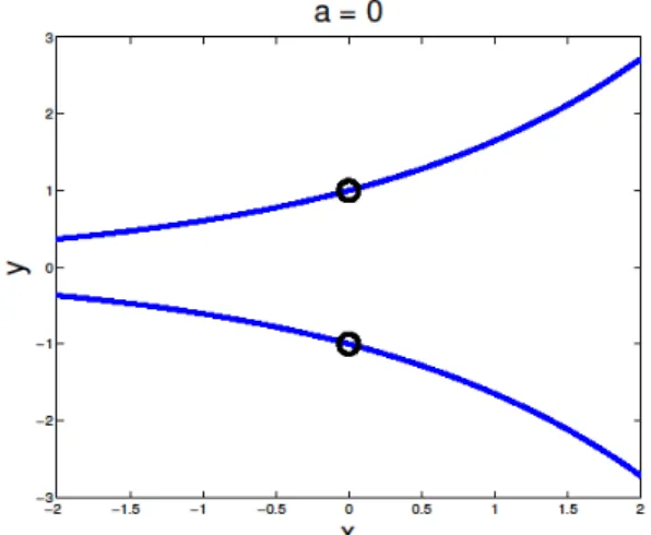
Figure 1. Illustration of problem (3) with = 0a . The two solutions, (0, 1) are indicated by black circles, and correspond to global minimizers. Starting from ( ,0),x₀ we observe x_k   and y_k 0 for all k. A typical SQP method will stop and claim to have found an optimal solution, with the help of a (very) large multiplier.

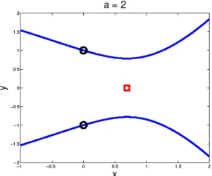
Figure 2. Illustration of problem (3) with a0. The (global) minimizers are (0, 1), indicated by black circles. The point indicated by a red square is a local maximizer. Starting from ( ,0),x₀ an SQP method will converge to the local maximizer.

Figures 1, 2 and 3 show the various situations graphically. Note that for all a R , Example 1 satisfies the linear independence constraint qualification at all feasible points. One of its features is that the inequality constraint is not active at the minimum of each inequality constrained problem.

(5)

THE SQUARED SLACKS TRANSFORMATION

25

Figure 3. Illustration of problem (3) with a0. The (global) minimizers are (0, 1), indicated by black circles. The point indicated by a red square is a critical point of the infeasibility measure. Using a starting point of the form ( ,0),x₀ an SQP method will converge towards the red square.

For the purpose of reference, note that the first-order optimality conditions of (1) are given by

 

0 and



,

 



0 . f x z c x z c x z c x            (4)

The main reason for the failure on Example 1 is the following. Assume that Problem (1) is regular in the sense that c x( ) 0*  at any critical point _{x Problem (2) is then regular as well and the Karush-Kuhn-Tucker}*_. conditions are necessary for first-order optimality. The Lagrangian for problem (2) is



_{, ,}



 



 

2



_,

L x y



f x 



c x y

where  is the Lagrange multiplier associated to the equality constraint, and at a first-order critical point, we must have

 

2 = 0 . f x c x y c x y   _ _{ }             (5) Note that in (5), the complementarity condition of (4) is only apparent as the equality



y = 0, so that the sign restrictions on the multiplier and on the constraints in the second part of (4) do not appear. As it turns out, the sign of the multiplier can be recovered from the second-order optimality conditions (see (Bertsekas, 1999, §3.3.2)). This pseudo-complementarity condition and the loss of sign restriction creates a difficulty in linearization-based methods. Indeed, any method that linearizes conditions (5) at a point ( , , )x y  will compute a step d = ( , , )d d d_x _y  satisfying

0 .

y

d yd y



 



 (6) Assume at some stage in the process we have y = 0 and 0. The linearization (6) then necessarily implies that d_y = 0. Thus, if ever y = 0 it will always remain equal to zero at subsequent iterations. Of course, if (1) is such that the constraint is inactive at x*, any method based on a linearization of (5) is bound to fail. Such is the

(6)

case with the examples of this section. A typical class of methods computing the step according to (6) is the class of SQP methods.

3. Numerical experiments

In order to eliminate side effects sometimes found in sophisticated implementations, we implemented a basic SQP method for equality-constrained problems, as given in (Nocedal and Wright, 1999, Algorithm 18.3), for example. The method is globalized with a backtracking linesearch on the L₁-penalty merit function

2 ( , )x yx y f xf x( )| ( )c xc x yy | , ( , )x y f x( ) | ( )c x y | , ( , ) ( ) | ( ) | , ( , )x y f x( ) | ( )c x y | , ( , ) ( ) | ( ) | , ( , )x y f x( ) | ( )c x y | , ( , ) ( ) | ( ) | ,

where  > 0 is a penalty parameter, and the Lagrange multipliers are updated using the least-squares estimates. In all cases, the starting point is chosen as (0,0) with the initial multiplier set to 1 2. In the following tables, k is the iteration number, ( ,x yk k) is the current iterate,



k is the current Lagrange multiplier estimate, Lk is the

gradient of the Lagrangian evaluated at ( ,x y_k _k, )



_k and



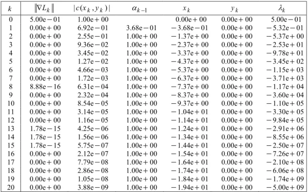
_k is the steplength computed from the backtracking linesearch.

Table 1. Iterations of the SQP method on problem (2) with = 0a

k Lk | ( ,c x yk k) |



k1 xk yk



k

0 5.00e



01 1 0.00e



00 2 0.00e



00 3 0.00e



00 4 0.00e



00 5 0.00e



00 6 0.00e



00 7 0.00e



00 8 8.88e



16 9 0.00e



00 10 0.00e



00 11 0.00e



00 12 0.00e



00 13 1.78e



15 14 1.78e



15 15 1.78e



15 16 0.00e



00 17 0.00e



00 18 0.00e



00 19 0.00e



00 20 0.00e



00 Table 1 gives the k. Because the the Lagrangian always attaining feasibility, This behaviour is 1.00e

00 0.00e

00 0.00e

00 5.00e

01 6.92e

01 3.68e

01

3.68e

01 0.00e

00

5.32e

01 2.55e

01 1.00e

00

1.37e

00 0.00e

00

5.37e

00 9.36e

02 1.00e

00

2.37e

00 0.00e

00

2.53e

01 3.45e

02 1.00e

00

3.37e

00 0.00e

00

9.78e

01 1.27e

02 1.00e

00

4.37e

00 0.00e

00

3.45e

02 4.66e

03 1.00e

00

5.37e

00 0.00e

00

1.15e

03 1.72e

03 1.00e

00

6.37e

00 0.00e

00

3.71e

03 6.31e

04 1.00e

00

7.37e

00 0.00e

00

1.17e

04 2.32e

04 1.00e

00

8.37e

00 0.00e

00

3.60e

04 8.54e

05 1.00e

00

9.37e

00 0.00e

00

1.10e

05 3.14e

05 1.00e

00

1.04e

01 0.00e

00

3.30e

05 1.16e

05 1.00e

00

1.14e

01 0.00e

00

9.84e

05 4.25e

06 1.00e

00

1.24e

01 0.00e

00

2.91e

06 1.56e

06 1.00e

00

1.34e

01 0.00e

00

8.55e

06 5.75e

07 1.00e

00

1.44e

01 0.00e

00

2.50e

07 2.12e

07 1.00e

00

1.54e

01 0.00e

00

7.26e

07 7.79e

08 1.00e

00

1.64e

01 0.00e

00

2.10e

08 2.86e

08 1.00e

00

1.74e

01 0.00e

00

6.06e

08 1.05e

08 1.00e

00

1.84e

01 0.00e

00

1.74e

09 3.88e

09 1.00e

00

1.94e

01 0.00e

00

5.00e

09 detail of the iterations in the case where = 0.a As expected, we see that y_k = 0 for all least-squares estimates happen to yield the exact multipliers in the present case, the gradient of vanishes. In order to satisfy the first-order optimality conditions, there thus only remains which is achieved by having

x

_k converge to . Note also that

|



_k

|

converges to . that of the first shortcoming of Section 2. Some backtracking linesearch iterations were only

(7)

THE SQUARED SLACKS TRANSFORMATION

27

necessary at the first iteration, the unit step was always accepted at the other iterations. Note that the fact that

k

x

'escapes' to  can be observed in practice by tightening the stopping tolerance.

Table 2 gives the detail of the iterations in the case where a= 1. The results are representative of any value < 0.a Here,

x

_k converges to a value which is a local maximizer. This illustrates the second shortcoming of Section 2. Again, no backtracking was necessary on this problem, except at the first iteration.

Table 2. Iterations of the SQP method on problem (2) with = 1a 

k Lk | ( ,c x yk k) |



k1 xk yk



k

0 1.00e



00 1.00e



00 0.00e



00 0.00e



00 5.00e



01 1 2.78e



17 5.68e



01 4.56e



01



2.28e



01 0.00e



00



1.27e



01 2 0.00e



00 3.59e



02 1.00e



00



5.44e



01 0.00e



00



3.44e



01 3 0.00e



00 1.49e



04 1.00e



00



5.67e



01 0.00e



00



3.62e



01 4 0.00e



00 2.56e



09 1.00e



00



5.67e



01 0.00e



00



3.62e



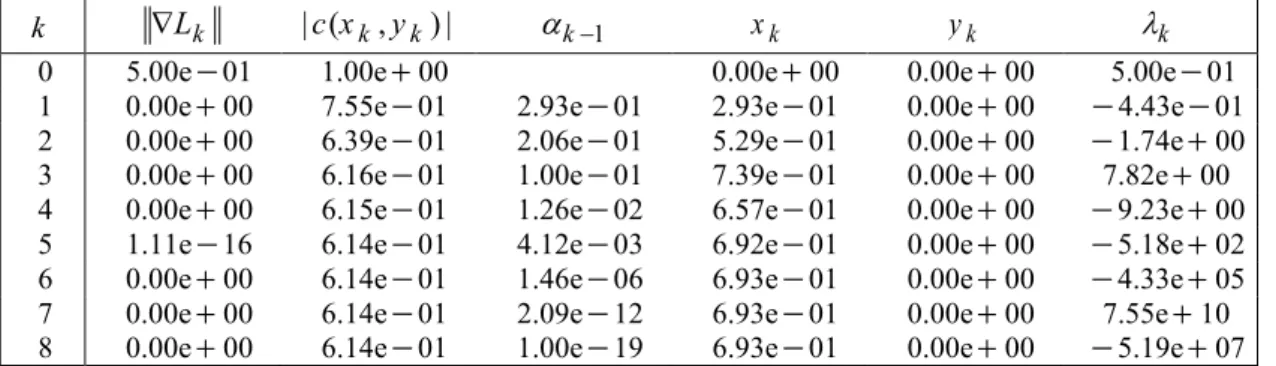
01

Table 3. Iterations of the SQP method on problem (2) with a= 2

k



L

k | ( ,c x yk k) |



k1 xk yk



k

0 5.00e



01 1.00e



00 0.00e



00 0.00e



00 5.00e



01 1 0.00e



00 7.55e



01 2.93e



01 2.93e



01 0.00e



00



4.43e



01 2 0.00e



00 6.39e



01 2.06e



01 5.29e



01 0.00e



00



1.74e



00 3 0.00e



00 6.16e



01 1.00e



01 7.39e



01 0.00e



00 7.82e



00 4 0.00e



00 6.15e



01 1.26e



02 6.57e



01 0.00e



00



9.23e



00 5 1.11e



16 6.14e



01 4.12e



03 6.92e



01 0.00e



00



5.18e



02 6 0.00e



00 6.14e



01 1.46e



06 6.93e



01 0.00e



00



4.33e



05 7 0.00e



00 6.14e



01 2.09e



12 6.93e



01 0.00e



00 7.55e



10 8 0.00e



00 6.14e



01 1.00e



19 6.93e



01 0.00e



00



5.19e



07 Finally, Table 3 gives the detail of the iterations in the case where = 2,a but again, the results are representative of any value a(0, ).e This situation is that given in the third shortcoming of Section 2. Backtracking was used in this case and the algorithm stopped claiming that the steplength was too small.

As a side note, we remark that when = ,a e there is a unique feasible point for (2) that has y = 0. The SQP algorithm convergestowards that point, which is in fact a saddle point. For > ,a e the feasible set is made of two disconnected curves. Each one intersects the axis y = 0. One of those intersection points is a local maximizer while the other one is a local minimizer, but neither of them has x = 0. Depending on the value of the starting point, the SQP algorithm converges to one or the other. We decided to not report those results here since they do not add new elements to the present analysis.

Finally, the above numerical results hold not only for an initial y₀= 0 but of course, also for y₀ sufficiently close to 0. This is an effect of finite precision however, and not a shortcoming of the SQP method.

4. Other algorithmic frameworks

As we showed in (6), any traditional SQP-type method will necessarily generate iterates of the form

( ,0)xk when started from ( ,0)x0 with a nonzero Lagrange multiplier. In this section, we show that similar conclusions hold for a variety of families of algorithms for nonlinear programming.

(8)

Augmented-Lagrangian-based methods fail for a reason similar to that given in Section 2. Note that the squared slacks transformation can again be used to derive the proper form of the augmented Lagrangian for inequality-constrained problems (Bertsekas, 1996, §3.1-3.2; Bertsekas, 1999, §4.2). Minimization of the augmented Lagrangian with squared slacks with respect to the slacks only yields the usual form for inequality-constrained problems. As we illustrate below, the direct application of the augmented Lagrangian algorithm to the formulation involving the slacks suffers the same pitfalls as the SQP method.

Consider the augmented Lagrangian for (2)



_{, , ;}



 



 

2



1



 

2



2_, 2

L x y   f x  c x y   c x y (7) where



> 0 is a penalty parameter and where  is the current estimate of the Lagrange multiplier. The step is computed from the Newton equations for (7), where



, , ;



 



_

,

  

_

2 , f x x y c x L x y y x y          _{ } _   (8) and





 





 

   

 





2 2 2 2 , 2 , , ; , 2 2 , 4 T T f x x y c x c x c x y c x L x y y c x x y y         _ _ _ _{ } _ _       _ _   

where



( , ) =x y

 

 ( ( )c x y2). In particular, the Newton equations yield 2

( ) _x ( ( , ) 2 ) _y = ( , )

y c x d x y y d y x y



  











where

d

_x and d_y are the search directions in x and y respectively. Whenever y = 0, the latter equation becomes



 

 c x d( )



_y = 0 ,

so that d_y = 0 provided that   c x( ) 0, or equivalently, provided that ( ,0) 0.x  Note, in the second component of (8), a 'complementarity' expression similar to that in the second component of (5).

The iterative minimization of (7) using the truncated conjugate gradient also preserves y = 0. Indeed, when started from

( ,0),

x

₀ the first search direction

p

₀ is the steepest descent direction and has the form

0

( ,0)



for some



₀R. The initial residual r₀ =p₀ thus will havethe same form and so will the next iterate

1 1 0 0 0

( , ) = (x y x 

 

,0) and the residual

r

₁

.

A property of the conjugate gradient method is that at the k-th iteration, the search direction p_k span{p_k_₁, }r_k (Golub and Loan, 1996, Corollary 10.2.4). Therefore p₁ necessarily shares the same form ( ,0).



₁ A recursion argument thus shows that the k-th conjugate-gradient iterate has the form ( ,0).



k This method will therefore also be unable to depart from the hyperplane y = 0.

5. Discussion

When the constraint of (1) is inactive, the optimal multiplier is = 0. However, in (2) we will frequently observe | |   when starting with y₀ = 0 to reach dual feasibility. Looking for instance at the results of Table 1, the final iterate ( 19.4,0) is feasible to within the prescribed tolerance. To compensate in dual feasibility, we need to have a large multiplier. In this sense, the addition of squared slacks has created a critical point at infinity.

For lack of a better initial value, implementations often set their variables to zero prior to starting the optimization, provided the objective and constraints are well defined at the origin. Modeling languages also often

(9)

THE SQUARED SLACKS TRANSFORMATION

29

set the variables to zero unless the user specifies otherwise. The difficulties exposed in this paper thus certainly occur in practice and illustrate another reason why starting points should not be chosen to be zero.

Unfortunately, the problem is difficult to avoid. Of course, it seems that we should not add squared slacks to convert inequality constraints into equality constraints. However problems having the form (2) where the variable y does not appear in the objective may arise in their own right. If at all feasible, it is recommended that equality constraints involving squared slack variables be convertedto inequality constraints.

It is worth noting that any problem of the form

 

,

x y f x c x g y 

where (0) = 0,g g(0) = 0 and g(0) 0 will exhibit a similar behavior. For instance, the functions ( ) = cosh( ),

g y y and ( ) = arctan( )g y  y dy have the desired properties. The objective may also have the form ( , )

f x y and the same conclusions hold if f x( ,0) /y = 0.

6. Acknowledgments

We are grateful to an anonymous referee for comments that improved the presentation of this paper.

7. References

BERTSEKAS, D. 1996. Constrained Optimization and Lagrange Multiplier Methods. Athena Scientific, Belmont MA, USA.

BERTSEKAS, D. 1999. Nonlinear Programming (2nd edition). Athena Scientific, Belmont MA, USA. BOGGS, P.T. and TOLLE, J.W. 1995. Sequential quadratic programming. Acta Numerica, 4: 1–51. GILL, P.E., MURRAY, W. and WRIGHT, M. 1981. Practical Optimization. Academic Press, London.

GOLUB, G.H. and VAN LOAN, C.F. 1996. Matrix Computations (3rd edition). Johns Hopkins University Press, Baltimore, MD, USA.

NASH, S.G. 1998. SUMT (Revisited). Operations Research, 46: 763–775.

NOCEDAL, J. and WRIGHT, S.J. 1999. Numerical Optimization. Springer series in Operations Research. Springer-Verlag, New York, USA.

TAPIA, R.A. 1980. On the role of slack variables in quasi-Newton methods for constrained optimization. In L.C.W. DIXON and G.P. SZEGÖ (eds.) Numerical Optimization of Dynamic Systems, pp. 235–246. North Holland Publishing Company.

Received 13 April 2011 Accepted 25 September 2011