Induced seismicity during the construction of the Gotthard Base Tunnel, Switzerland: hypocenter locations and source dimensions

ORIGINAL ARTICLE

Induced seismicity during the construction of the Gotthard

Base Tunnel, Switzerland: hypocenter locations

and source dimensions

Angela von Deschwanden

Received: 28 June 2011 / Accepted: 28 November 2011 / Published online: 21 June 2012 # Springer Science+Business Media B.V. 2012

Abstract A series of 112 earthquakes was recorded between October 2005 and August 2007 during the excavation of the MFS Faido, the southernmost access point of the new Gotthard Base Tunnel. Earthquakes were recorded at a dense network of 11 stations, including 2 stations in the tunnel. Local magnitudes computed from Wood–Anderson-filtered horizontal component seismograms ranged from −1.0 to 2.4; the largest earthquake was strongly felt at the surface and caused considerable damage in the tunnel. Hypo-center locations obtained routinely using a regional 3-D P-wave velocity model and a constant Vp/Vs ratio

1.71 were about 2 km below the tunnel. The use of seismic velocities calibrated from a shot in the tunnel revealed that routinely obtained hypocenter locations were systematically biased to greater depth and are now relocated to be on the tunnel level. Relocation of the shot using these calibrated velocities yields a location accuracy of 25 m in longitude, 70 m in latitude, and 250 m in focal depth. Double-difference relative relocations of two clusters with highly similar waveforms showed a NW–SE striking trend that is consistent with the strike of mapped faults in the MFS Faido. Source dimensions computed using the quasidynamic model of Madariaga (Bull Seismo Soc Am 66(3):639–666, 1976) range from 50 to 170 m. Overlapping source dimensions for earthquakes within the two main clusters suggests that the same fault patch was ruptured repeatedly. The observed seismic-ity was likely caused by stress redistribution due to the excavation work in the MFS Faido.

Keywords Induced seismicity . Earthquake locations . Source dimensions . Gotthard Base Tunnel . Stress redistribution

1 Introduction

With a length of 57 km, the Gotthard Base Tunnel forms the centerpiece of the New Alpine Traverse through the Swiss Alps. The northern entry point is at the village Erstfeld, at the southern tip of Lake Lucerne; it ends at the village Biasca in the Ticino DOI 10.1007/s10950-012-9313-8

An earlier version of this article was published in Volume 16, Issue 2, under DOI 10.1007/s10950-011-9261-8.

S. Husen (*)

Swiss Seismological Service, ETH Zurich, Sonneggstrasse 5,

CH 8092 Zurich, Switzerland e-mail: husen@sed.ethz.ch

E. Kissling

Institute of Geophysics, ETH Zurich, Sonneggstrasse 5,

CH 8092 Zurich, Switzerland

A. von Deschwanden

Institute of Geophysics, ETH Zurich, Sonneggstrasse 5,

CH 8092 Zurich, Switzerland

Present Address: A. von Deschwanden

Norwegian Polar Institute, Polar Environmental Centre, Tromsø 9296, Norway

(Fig. 1). The Gotthard Base Tunnel is designed as a railway tunnel for passenger and freight trains, con-sisting of two single tracks, each with a diameter of 9.2 m. Three intermediate access points divide the tunnel into five sections with about equal length. The southernmost of these access points, called MFS Faido, is located near the village of Faido in the Ticino (Fig.1). It is designed to serve as an emergency access point to evacuate train passengers in case of emergen-cies. Therefore, the layout of the MFS Faido consists of several parallel and crossing tubes (Fig.2). Exca-vation was done by drilling and blasting, starting in February 2002; main excavation work of the MFS Faido was finished by October 2006.

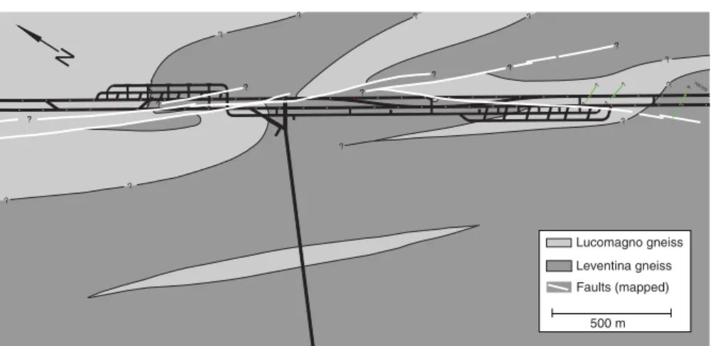
The Gotthard Base Tunnel crosses the central Alps. It is located mainly in igneous rocks consisting of the Aare and Gotthard massifs in the north and in meta-morphic rocks of the Penninic nappes in the south. Geology in the MFS Faido is dominated by the contact between the Lucomagno and Leventina gneisses, which are part of the Penninic nappes. The contact zone forms a complex three-dimensional structure

(Fig. 2). In terms of rheology, these two gneisses behave differently: At the depth of the tunnel, the Lucomagno gneiss deforms more ductile, whereas the Leventina gneiss deforms more brittle. During excavation, a complex fault zone was encountered in the northern part of the MFS Faido (Fig.2). The fault zone strikes about NW–SE with a dip of about 80°. Rocks of the fault zone are heavily fractured, includ-ing kakitrite in the fault kernel.

Excavation of the MFS Faido was accompanied by large deformation and extensive and strong rock burst activity. The majority (75%) of rock bursts occurred close to the active rockface, within 3 h after blasting (Hagedorn and Stadelmann 2010). Large rock bursts also occurred repeatedly in sections, where excavation work was already finished. These sections located in the northern part of the MFS Faido, in the complex contact zone of the Lucomagno and Leventina gneisses (Fig.2). Rock bursts were sometimes accom-panied with spalling of shotcrete, threatening work-people in the tunnel. Between March 2004 and October 2005, the Swiss Seismological Service

Faido FUSIO MUO BNALP Biasca Sedrun Erstfeld Gotthard basetunnel 5 km Ml=2.0 SDSNet Ml=1.0 Earthquakes Stations Fig. 1 Map of study area.

Gray circles mark

seismicity as recorded by the Swiss Digital Network (SDSNet) between 1995 and 2005; red circles mark earthquakes in the vicinity of the village Faido between 2004 and 2005. Size of the circles scales with magnitude. Permanently installed stations of the SDSNet are shown by black triangles. Green dashed line marks location of the Gotthard Base Tunnel. Inset in upper right corner shows location of the study region within Switzerland

recorded 12 small earthquakes (ML 0.9–1.6) in the vicinity of the village of Faido (Fig.1). Prior to March 2004, no earthquakes were recorded in this area (Baer et al.2005). Hypocenter locations of these earthquakes were poorly constrained due to the low number of stations of the Swiss Digital Seismic Network (SDSNet) that recorded the events. Only station FUSIO of the SDSNet was within 10 km distance of the epicenters of the events (Fig. 1). Three of the recorded earthquakes could be correlated with the occurrence of large rock bursts in the tunnel, suggest-ing that the observed seismicity was related to the construction of the MFS Faido. In order to monitor ongoing seismicity in the vicinity of the MFS Faido and to study possible mechanisms that caused the observed earthquake activity, a dense seismic network of 10 stations was installed and operated by the Swiss Seismological Service in the region of Faido. The work was done under a contract given by the AlpTran-sit Gotthard AG, the owner of Gotthard Base Tunnel. In this study, we will describe the installation and operation of the AlpTransit seismic network, present our results in terms of hypocenter locations and source dimensions, and discuss possible mechanisms that caused the observed seismicity.

1.1 AlpTransit network

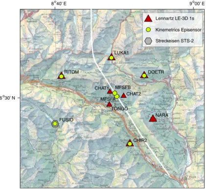
In order to monitor the seismicity in the vicinity of the MFS Faido, a dense network of seismic stations was installed between October 2005 and December 2005, with the exception of station MFSFB, which was installed in November 2006 (Fig. 3). The AlpTransit network was operated between October 2005 and

April 2010 by the Swiss Seismological Service (SED) at ETH Zurich, under a contract with AlpTran-sit Gotthard AG. The design of the network consisted of an inner circle with a diameter of 1–2 km (stations CHAT1, CHAT2, and TONGO) and an outer circle with a diameter of 10–12 km (stations CHIR2, DOETR, FUSIO, LUKA1, NARA, RITOM) centered on the MFS Faido. In addition, two stations (MFSFA and MFSFB) were installed within the MFS Faido (Fig.3). The majority of stations were equipped with short-period seismometers (Lennartz LE-3-D 1 s), ex-cept for stations FUSIO, MFSFA, and MFSFB. Sta-tion FUSIO belongs to the SDSNet, a permanently operated network by SED, and is, therefore, equipped with broadband seismometer (Streckeisen STS-2). Due to the expected high-noise level in the tunnel and due to the small epicentral distances, stations MFSFA and MFSFB were equipped with 24-bit accel-erometers (Kinemetrics EpiSensor).

Data were recorded continuously at sampling fre-quencies of 120 Hz (FUSIO), 200 Hz (CHAT1, CHAT2, CHIR2, DOETR, FUSIO, LUKA1, NARA, RITOM, TONGO), and 250 Hz (MFSFA and MFSFB). Except for station LUKA1, all data were streamed in real time to the SED data center in Zurich using high-speed internet connections. Data from sta-tion LUKA1 were manually downloaded and merged to existing data since the bandwidth of the internet connection at station LUKA1 was not sufficient to allow for real-time data streaming. All stations were synchronized using GPS timing. Unfortunately, a soft-ware bug caused timing problems at stations CHIR1, DOETR, NARA, RITOM, and TONGO between Oc-tober and November 2005. Consequently, arrival times ? ? ? ? ? ? ? ? ? ? ? ? ? ? ? ? N 705’000 ? 706’000 ? ? ? ? ? Lucomagno gneiss Leventina gneiss Faults (mapped) 500 m Fig. 2 Geologic map of the

multifunction station MFS Faido. Lucomagno and Leventina gneisses are shown by light and dark gray colors, respectively. White lines mark mapped faults in the MFS Faido (Hagedorn and Stadelmann 2010). Black lines denote tunnel layout of the MFS Faido

picked at these stations between October and November 2005 were not used for earthquake location; amplitudes were still used to compute local magnitudes.

2 Routine data analysis

2.1 Hypocenter locations and local magnitudes Event detection was based on short-time/long-time (STA/LTA) amplitude ratios computed continuously on the incoming data streams of the AlpTransit sta-tions. An event was declared if the STA/LTA ampli-tude ratio exceeded a given threshold at two or more stations within time window of 40 s. For each event, waveform data of 90 s length from stations of the AlpTransit network and nearby broadband stations of the SDSNet were extracted from the continuous data streams. Each event file was manually checked and false events were removed. This resulted in 112 earth-quakes detected by the AlpTransit network between October 2005 and August 2007.

Arrival times of P- and S-waves were picked man-ually by experienced seismologists at the SED. All data were band-passed filtered in the frequency band 1–30 Hz to ensure a uniform signal character as much

as possible. Moreover, band-passed filtering sup-pressed acausal finite impulsive response filter arti-facts which were sometimes present at nearby stations (CHAT1, CHAT2, MFSFA, and MFSFB) due to very impulsive arrivals of the direct P-wave (Scherbaum and Bouin1997). Uncertainties in arrival times were assigned using a quality weighting scheme with uncertainties ranging from 0.05 s (quality 0) to 0.4 s (quality 3) (Table 1). The majority of P-wave arrival times were of quality 0 due to high signal-to-noise ratios and a high-frequency content of the phase arrivals (Table3).

Earthquakes were routinely located using a regional 3-D P-wave velocity derived from local earthquake tomography and controlled-source seismology data (Husen et al. 2003) and the NonLinLoc software package (Lomax et al.2000). A constant Vp/Vs ratio

9 00’ E 8 40’ E 46 30’ N TONGO MFSFA MFSFB CHAT1 CHAT2 CHIR2 FUSIO NARA LUKA1 DOETR RITOM Streckeisen STS-2 Lennartz LE-3D 1s Kinemetrics Episensor

Fig. 3 Map of the AlpTransit seismic network. Different sensor types are marked by different symbols as indicated. Station FUSIO belongs to the Swiss Digital Seismic Network. White line marks location of the Gotthard Base Tunnel

Table 1 Uncertainty assessment for arrival time picking

Class Uncertainty Number of

P-wave picks Number of S-wave picks 0 ±0.025 s 834 271 1 ±0.05 s 71 144 2 ±0.1 s 12 89 3 ±0.2 s 3 5

of 1.71 was used for S-wave arrivals. NonLinLoc computes the posterior probability density function (pdf) of the earthquake location problem (Tarantola and Valette1982) using an importance sampling algo-rithm, called OctTree search (Lomax and Curtis2001). The solution includes uncertainties due to the geome-try of the network, measurements errors of the ob-served arrival times and errors in the calculation of theoretical travel times. These uncertainties are repre-sented either as density scatter plots (Lomax et al.

2000) or as traditional 68% confidence ellipsoids. In the case of well-constrained hypocenter locations, the 68% confidence ellipsoid is a valid approximation of the posterior pdf (Lomax et al.2000). Figure4shows hypocenter locations for earthquakes with an azimuth-al gap less than 160° and with a length of the major axis of the 68% confidence ellipsoid less than 3 km.

Average length of the major axis of the 68% confi-dence ellipsoid was 1.9 km.

Local magnitudes (ML) were computed using max-imum amplitudes of the Wood–Anderson-filtered hor-izontal component seismograms. The final magnitude for one event corresponds to the median of all station magnitudes. The distance attenuation relationship used at SED was originally derived using vertical recordings on short-period instrumentation with ana-logue telemetry (Kradolfer 1984). After updating to the modern SDSNet an empirically derived correction factor of−0.1 is applied to maintain consistency in the MLscale (Edwards et al. 2010). The distance attenu-ation relattenu-ationship used at SED is not well-calibrated for distances <30 km as many of the signals used in the calibration at that time were clipped in this dis-tance range due to the limited dynamic range of ana-logue telemetry. Nevertheless, we decided to use the SED MLscale, but we did not compute magnitudes at stations MFSFA and MFSFB since their locations are generally less than 1 km from the epicenter locations of the earthquakes. Our magnitudes may, therefore, be over- or underestimated compared to the SED ML scale, but they are internally consistent as more or less the same set of stations is used for computation. A few earthquakes were too small to be recorded at stations on the surface; they were only recorded at stations MFSFB and MFSFA in the tunnel. Magnitudes for these events were computed using amplitude ratios of Wood– Anderson-filtered and integrated horizontal component seismograms at station MFSFA for a reference M1.0 earthquake and each event. The magnitude of the refer-ence event was computed using the surface stations of the network as described above. In principle, the spectral fitting method described in Section 5 would allow to compute moment magnitudes Mwfor small earthquakes (Edwards et al.2010). Due to quality constraints (main-ly signal-to-noise ratio and azimuthal distribution of stations) moment magnitudes could only be computed for 53 out of 112 events. We, therefore, decided to use MLinstead of Mwin our study to have a more complete record of magnitudes over time.

2.2 Calibration shot

Routinely obtained earthquake locations clustered in the vicinity of the MFS Faido but they located 2 km below the tunnel (Fig. 4). Focal depths were well constrained due to the excellent network geometry

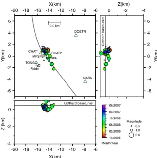
-20 -18 -16 -14 -12 -10 -8 -6 X(km) -20 -18 -16 -14 -12 -10 -8 -6 X(km) -20 -18 -16 -14 -12 -10 -8 -6 X(km) -20 -18 -16 -14 -12 -10 -8 -6 X(km) -20 -18 -16 -14 -12 -10 -8 -6 X(km) -20 -18 -16 -14 -12 -10 -8 -6 X(km) -20 -18 -16 -14 -12 -10 -8 -6 X(km) Z(km) -20 -18 -16 -14 -12 -10 -8 -6 X(km) -6 -4 -2 0 2 4 6 Y(km) -6 -4 -2 0 2 4 6 Y(km) -6 -4 -2 0 2 4 6 Y(km) -6 -4 -2 0 2 4 6 Y(km) -6 -4 -2 0 2 4 6 Y(km) -6 -4 -2 0 2 4 6 Y(km) -6 -4 -2 0 -4 -2 0 2 4 6 Y(km) Z (km) -6 -4 -2 0 2 4 6 Y(km) -6 -4 -4 -2 -2 0 0 2 4 6 Y(km) Gotthard basetunnel Gotthard basetunnel 10/2005 Month/Year 02/2006 06/2006 10/2006 02/2007 06/2007 0.5 1.0 2.0 Magnitude 2.0 km Faido MFSFA MFSFB CHAT1 _CHAT2 TONGO NARA DOETR

Fig. 4 Hypocenter locations of earthquakes in the vicinity of the MFS Faido between October 2005 and June 2007. Map view and two vertical cross-sections along X- and Y-axis are shown. Only events with GAP <160° and length of the major axis of the 68% confidence ellipsoid <3 km are shown. Earthquake loca-tions were obtained using regional 3-D P-wave velocity model (Husen et al.2003) and a constant Vp/Vs ratio of 1.71. Origin time of earthquakes is coded by color as indicated. Circle size is scaled by magnitude as indicated. Locations of stations of the AlpTransit seismic network are marked by triangles. Square marks location of the town of Faido. Black line marks location of the Gotthard Base Tunnel. Thin black lines in the vertical cross-sections mark elevation of the Gotthard basetunnel. Note that earthquakes locate on average 2 km below the Gotthard Base Tunnel

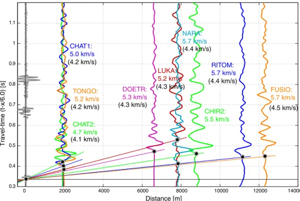
for most earthquakes as indicated by the small size of the 68% confidence ellipsoid. Large P-wave ampli-tudes on the horizontal components of station MFSFA, however, suggested that earthquakes likely occurred at the depth of the tunnel (i.e., 400 m above sea level). Moreover, S–P arrival times at station MFSFA were less than 0.1 s indicating that the earthquakes located at a distance of only a few hundred meters from station MFSFA. All this suggests that hypocenter locations obtained using the regional 3-D P-wave model and a constant Vp/Vs ratio were likely biased to greater depth. In order to check the reliability of the regional 3-D P-wave velocity model and to assess location accuracy of the obtained hypocenter locations, a cali-bration shot was fired on November 9, 2006. The shot was set off in southern part of the MFS Faido; the charge was 100 kg explosive. A Kinemetrics EpiSen-sor was installed at about 30 m distance to the shot point to record the origin time of the shot. The shot was well recorded at all stations of the AlpTransit network (Fig. 5). Average P-wave velocities were

computed for each station using the arrival time of the direct P-phase. Overall, seismic velocities were about 20% faster than the corresponding P-wave ve-locities taken from the 3-D P-wave velocity model. Moreover, seismic velocities derived from the calibra-tion shot showed large local variacalibra-tions between 4.7 and 5.7 km/s, which were not present in the regional 3-D P-wave velocity model (Fig.5).

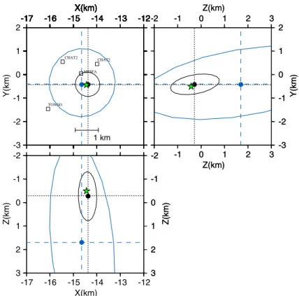
We relocated the calibration shot using seismic veloc-ities taken from the regional 3-D P-wave velocity model and derived from the shot itself (Fig.6). For the latter, we used a smaller model error in NonLinLoc as uncertain-ties in seismic velociuncertain-ties derived from the calibration shot are much smaller than for those taken from the 3-D P-wave velocity model. As a consequence, location uncertainties (as shown by the 68% confidence ellipsoid in Fig.6) are significant smaller. It should be noted that model uncertainty estimates as used for the calibration shot will likely not reflect all expected velocity hetero-geneity. A more complete uncertainty estimate, however, could only be achieved by placing calibration shots next

0 2000 4000 6000 8000 10000 12000 14000 0.3 0.4 0.5 0.6 0.7 0.8 0.9 1 1.1 Distance [m] Travel-time (t-x/6.0) [s] CHAT2: 4.7 km/s CHAT1: 5.0 km/s (4.2 km/s) (4.2 km/s) (4.3 km/s) (4.3 km/s) (4.5 km/s) (4.4 km/s) (4.4 km/s) (4.1 km/s) TONGO: 5.2 km/s DOETR: 5.3 km/s LUKA: 5.2 km/s NARA: 5.7 km/s CHIR2: 5.5 km/s RITOM: 5.7 km/s FUSIO: 5.7 km/s

Fig. 5 Travel time diagram of calibration shot. Travel times are reduced by 6 km/s. Waveforms of different stations of the AlpTransit seismic network are shown by different colors as indicated. Waveform of the station close to the calibration shot is shown in gray. Name and average P-wave velocity for each station as estimated from the slope of the corresponding travel

time curves is indicated. Corresponding P-wave velocity as estimated from the regional 3-D P-wave velocity model (Husen et al.2003) is shown in brackets. P-wave velocities as estimated from the regional 3-D P-wave velocity model are on average 1 km/s slower

to the earthquake source region, which was not realistic in the scope of this study. Using calibrated seismic velocities for each individual station, the calibration shot was relocated within 25 m in X-direction, 70 m in Y-directon, and 250 m in Z-direction of the true location (Fig.6). Using the regional 3-D P-wave velocity model, the calibration shot was relocated within 200 m in X-direction, 200 m in Y-X-direction, and 2,100 m in Z-direc-tion. Hence, earthquake locations computed using the regional 3-D P-wave model were biased to greater depth due to the use of inadequate seismic velocities. Conse-quently, all earthquakes were relocated using calibrated seismic velocities for each individual station (Fig.7). 2.3 Temporal and spatial evolution of observed seismicity

In total, 112 earthquakes were detected and located by the network between October 2005 and August 2007.

Figure8shows the temporal evolution of the seismicity. Seismic activity was highest in the months December 2005, March 2006, and May 2006. Overall, seismicity decayed over time and no earthquake was recorded after August 2007 (Fig. 8), about 5 months after the main excavation work was finished in the MFS Faido. Local magnitudes ranged between −1.0 and 2.4 (Fig. 8). It should be noted that negative magnitudes are only based on amplitude ratios at station MFSFA as discussed in Section3.1. Hence, these magnitudes should be inter-preted carefully. The largest earthquake with ML02.4 occurred on March 25, 2006. It was strongly felt by local people in nearby villages and caused intensive media interest. The fact that the earthquake was strongly felt at the surface is likely due to its shallow focal depth. The earthquake occurred at a depth 0.5–1.0 km below the Earth’s surface. No damage was reported at the surface, but the earthquake caused considerable damage in the MFS Faido, including cracking and massive

Z(km) -2 -1 0 1 2 3 Z(km) -2 -1 0 1 2 3 -2 -1 0 1 2 3 Z(km) -17 -16 -15 -14 -13 -12 X(km) 0 Y(km) -17 -16 -15 -14 -13 -12 X(km) MFSFA -17 -16 -15 -14 -13 -12 X(km) CHAT2 -17 -16 -15 -14 -13 -12 X(km) -17 -16 -15 -14 -13 -12 X(km) CHAT2 -17 -16 -15 -14 -13 -12 X(km) TONGO -17 -16 -15 -14 -13 -12 X(km) -17 -16 -15 -14 -13 -12 X(km) -17 -16 -15 -14 -13 -12 X(km) -17 -16 -15 -14 -13 -12 X(km) -17 -16 -15 -14 -13 -12 X(km) -17 -16 -15 -14 -13 -12 X(km) -17 -16 -15 -14 -13 -12 X(km) -17 -16 -15 -14 -13 -12 X(km) -3 -2 -1 1 2 -17 -16 -15 -14 -13 -12 X(km) 1 km -3 -2 -1 0 1 2 Y(km) -1 0 1 2 3 Z(km) -2 -1 0 1 2 3 Z(km) -3 -2 -1 0 1 2 Y(km) -1 0 1 2 3 Z(km) -2 -1 0 1 2 3 Z(km)

Fig. 6 Hypocenter locations of relocated calibration shot. Blue circles and blue dashed lines mark hypocenter location comput-ed using regional 3-D P-wave velocity model (Husen et al. 2003); black circles and black lines mark hypocenter location computed using average P-wave velocities for each stations as estimated from the calibration shot. Projection of the corresponding 68% confidence ellipsoid is shown in blue and

black, respectively. Smaller model uncertainties for calibrated velocities yield a smaller size of the 68% confidence ellipsoid. True location of the calibration shot is marked by green star. Location of stations of the AlpTransit seismic network is marked by squares. Using the regional 3-D P-wave velocity model, calibration shots locate 2 km deeper than the true location

flaking of the reinforced tunnel walls, and uplift of about 0.5 m of the tunnel floor.

The ML 2.4 earthquake was well recorded at all stations of the AlpTransit network and of the SDSNet, up to distances of 140 km. The excellent azimuthal and spatial distribution of the observations allowed us to compute a focal mechanism based on first motions (Fig.9). Take-off angles were computed for the regional

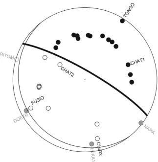
3-D P-wave velocity model (Husen et al.2003) at the hypocenter location computed using only stations of the AlpTransit network and calibrated seismic velocities as discussed in the previous section. As can be inferred from Fig.9, fault planes of the focal mechanism are well constrained by our observations. First motions observed at stations DOETR, LUKA1, and NARA seem to be inconsistent with obtained focal mechanism. These dis-crepancies can be due to incorrectly computed take-off angles for these stations, which were computed as up-ward. The shallow depth of the event (focal depth is about 1 km below the Earth’s surface) and significant surface topography in the region, however, could result in downward oriented take-off angles for these stations, which would be consistent with the obtained focal mechanism. Strike and dip of one of the fault planes of the focal mechanism of the ML2.4 earthquake is con-sistent with strike and dip of the mapped fault zone in the MFS Faido. We, therefore, interpret the focal mech-anism of the ML2.4 earthquake as a NW–SE oriented, steeply dipping normal fault event that likely occurred on one of the faults belonging to the fault system mapped in the MFS Faido (Fig.2).

3 High-precision earthquake relocation 3.1 Improving arrival time picks by waveform cross-correlation

Routine data analysis revealed earthquakes with a high degree of waveform similarity suggesting that these

-20 -18 -16 -14 -12 -10 -8 -6 X(km) Z(km) -20 -18 -16 -14 -12 -10 -8 -6 X(km) -6 -4 -2 0 -4 -2 0 2 4 6 Y(km) Z (km) -6 -4 -4 -2 -2 0 0 2 4 6 Y(km) Gotthard basetunnel Gotthard basetunnel 10/2005 Month/Year 02/2006 06/2006 10/2006 02/2007 06/2007 0.5 1.0 2.0 Magnitude 2.0 km Faido MFSFA MFSFB CHAT1 _CHAT2 TONGO NARA DOETR

Fig. 7 Hypocenter locations of earthquakes in the vicinity of the MFS Faido between October 2005 and June 2007 (same layout as Fig.4). Only events with GAP <160° and length of the major axis of the 68% confidence ellipsoid <3 km are shown. Earthquake locations were obtained using calibrated P-wave velocities. Note that earthquakes locate on average at the same depth as the Gotthard Base Tunnel

0.5 0.0 -0.5 -1.0 1.0 1.5 2.0 2.5 Magnitude (ML)

Oct Dec Feb Apr Jun Aug Oct Dec Feb

Month Month

Apr Jun Aug Oct Dec

2005 2006 2006 2007 2007

Oct

2005 2006 2006 2007 2007

Dec Feb Apr Jun Aug Oct Dez Feb Apr Jun Aug

Month Month 0 5 10 15 20 Number Oct Dec Fig. 8 Temporal evolution

of the observed seismicity between October 2005 and December 2007. Top panel shows number of events per month; bottom panel shows local magnitudes (ML) per month. Open circles mark earthquakes for which ML could only be computed using recordings of station MFSFA. Thick gray line marks the end of the excavation work in the MFS Faido (October 2006)

events occurred very close to each other with similar source mechanisms. We, therefore, performed a cluster analysis based on waveform similarity to identify fam-ilies of similar earthquakes. Following the cluster anal-ysis, cross-correlation times within each family are then used to improve consistency of absolute arrival times. Such an approach has been shown to significantly reduce location scatter, which is often introduced by the variability in picking arrival times on an event-by-event basis (Rowe et al. 2004,2002b). Details on the techniques used for waveform cross-correlation and clustering can be found in Rowe et al. (2002a). The goal of the cluster analysis is to obtain families with similar waveforms in order to improve arrival times by cross-correlation. This is in contrast to other clustering techniques that aim at identifying clusters of mostly identical waveforms. For these reasons, we based our cluster analysis only on one station (DOETR) with an almost complete record of the observed seismicity and high signal-to-noise ratios. Waveforms were filtered using a 1–10 Hz bandpass filter prior to waveform

cross-correlation. A window length of 2 s, starting 0.4 s before the routinely determined P-wave arrival time, was chosen for cross-correlation. This window length included the arrivals of P- and S-wave energy. Finally, a cross-correlation coefficient of 0.9 was cho-sen as a cutoff for clustering. The goal of these pa-rameter settings was to establish families with highly similar waveforms. A shorter window length includ-ing only the P-wave arrival, for example, would have yielded a larger number of waveforms with higher cross-correlation coefficients but not necessarily more reliable results as scattering effects and the arrival of the S-wave would have not be considered. The cluster analysis revealed 12 clusters, of which two clusters contained a larger number of earthquakes (clusters 11 and 12; Table2). The ML2.4 earthquake of March 25, 2006, is associated with cluster 11, which consists of 16 earthquakes and is the largest cluster.

Following the cluster analysis, arrival times of earthquakes in clusters 11 and 12 were refined using cross-correlation time lags for each station following the approach of Rowe et al. (2002a). Arrival times of earth-quakes in the remaining clusters were not adjusted, as the number of events per cluster was too low. Stations with a good signal-to-noise ratio (e.g., station DOETR in Fig.10) showed only a minor improvement in pick consistency. Pick improvement was considerable for stations with a low signal-to-noise ratio (e.g., station NARA in Fig.10), demonstrating that arrival time picks at stations with a low signal-to-noise ratio suffer from a strong variability. Following the pick adjustment, traces were stacked for each station and cluster to check for a mean bias in adjusted arrival times. Moreover, pick uncertainties were estimated for each stack following the concept of earliest and latest possible arrival times, i.e., the difference between earliest and latest possible arrival time determines absolute pick uncertain-ty (Diehl et al.2009). Pick uncertainties derived from the stacks were a factor of 4–5 smaller than the corresponding uncertainties derived during routine pick-ing due to an improved signal-to-noise ratio of the stacks. Figure 11 shows hypocenter locations of earth-quakes in cluster 12 as computed by NonLinLoc and using velocities as estimated from the calibration shot. The improvement in picking consistency yields a tight clustering in epicenter location and focal depth. Loca-tion uncertainties as outlined by the 68% confidence ellipsoid were also slightly reduced due to reduced picking uncertainties as estimated from the stacks

CHAT2 CHAT1 TONGO DOETR LUKA1 NARA CHIR2 RITOM FUSIO

Fig. 9 Fault plane solution of the ML 2.4 earthquake of March 25, 2006, based on first-motion polarities. Shown is equal-area, lower-hemisphere projection. Preferred rupture plane is shown by thick black line. Solid circles correspond to compressive first motion (up) and open circles to dilatational first motion (down). Observations from the stations of the AlpTransit seismic net-work are labeled. Mismatch between observed and computed first motion at stations RITOM, LUKA1, and NARA can be caused by erroneous take-off angle computations. See text for more details

(Fig.11). Nevertheless, the size of the location uncer-tainties prevents interpretation of the internal structure of the cluster, i.e., whether all earthquakes occurred at the same location or not.

3.2 Double-difference hypocenter locations

In order to improve our resolution to resolve any internal structure, we relocated earthquakes of clusters 11 and 12 using hypoDD (Waldhauser and Ellsworth

2000). Initial locations were computed by NonLinLoc using either original arrival time picks or refined ar-rival time picks. Since the original version of hypoDD does not account for station elevations, we modified hypoDD accordingly. Neglecting station corrections in hypoDD does not pose a problem as long as focal depths are large compared to epicentral distance. For these cases, changes in the take-off angles are small if station elevations are used or not. In our study, how-ever, where seismicity is very shallow and stations in the tunnel are nearly at the same elevation as the seismicity, the use of station elevations becomes cru-cial to compute correct take-off angles. We used a velocity model with a constant P-wave velocity of 5.33 km/s, which corresponds to the average velocity of all stations in the AlpTransit network as estimated by the calibration shot. Only P-wave arrival times of stations in the AlpTransit network were consequently used for relocation. Among network geometry, the

power of hypoDD to resolve small structures depends on uncertainties and consistencies of the arrival times. Therefore, cross-correlation measurements are often combined with catalog picks to improve hypoDD locations (e.g., Waldhauser and Ellsworth 2000; Richards et al. 2006). This approach requires careful and sophisticated weighting between the two sets of arrival times. In this study, we used only one set of arrival times, which were either derived from routine picking (catalog picks) or from the pick refinement as outlined above. The latter set of arrival times inher-ently contains information from cross-correlation measurements, as they were used to refine the picks. The advantage of our approach is that no sophisticated weighting scheme is needed as only one set of arrival times is used. We stop hypocenter relocation in hypoDD when the final RMS of all travel time resid-uals reaches our assumed average picking uncertainty (20 ms for original picks and 6 ms for refined picks). Compared to original locations obtained by NonLin-Loc, hypocenter locations show a much tighter clus-tering when they are relocated by hypoDD (Fig. 12). Location scatter is further reduced if the refined picks are used. Location uncertainties as computed by hypoDD are in the range of 30–60 m for catalog picks and 10–20 m for the refined picks, respectively. Since hypoDD scales formal location uncertainties by the final traveltime residual, smaller uncertainties can be expected if the refined picks are used for relocation. Table 2 Results of cluster analysis using waveform cross-correlation

Cluster Number of events Mean cross-correlation coefficient Standard deviation of cross-correlation coefficient Minimum cross-correlation coefficient Maximum cross-correlation coefficient 0 33 0.0490 0.0001 0.0490 0.0490 1 3 0.9883 0.0075 0.9830 0.9990 2 4 0.9750 0.0099 0.9570 0.9880 3 3 0.9527 0.0117 0.9370 0.9650 4 2 0.9280 0.0000 0.9280 0.9280 5 2 0.9270 0.0000 0.9270 0.9270 6 2 0.9180 0.0000 0.9180 0.9180 7 3 0.9210 0.0085 0.9090 0.9280 8 2 0.9110 0.0000 0.9110 0.9110 9 2 0.9010 0.0000 0.9010 0.9010 10 2 0.9000 0.0000 0.9000 0.9000 11 16 0.9530 0.0215 0.9040 0.9910 12 9 0.9017 0.2086 0.0490 0.9930

3.3 Assessing double-difference location uncertainties using synthetic data

The reliability of location uncertainties computed by hypoDD needs to be checked by statistical sampling techniques, such “bootstrap” or “jacknife” tests, to assess the influence of the network geometry on the location uncertainties (Waldhauser and Ellsworth

2000). In our study, we performed tests with synthetic data to assess location uncertainties. Synthetic travel-times are computed for each observation within clus-ters 11 and 12 using the same velocity model used for relocation in hypoDD (i.e., a constant P-wave velocity

of 5.33 km/s). For each cluster, all earthquakes origi-nate at the same location (Fig. 13). Gaussian distrib-uted errors are added to the synthetic traveltimes to model pick uncertainties. We use standard deviations of 0.025 and 0.01 s to simulate pick uncertainties for routine picks and refined picks, respectively. Our syn-thetic data are, therefore, as close as possible to the observed data but using known (or“true”) hypocenter locations. Figure13shows the results using both syn-thetic datasets. As expected, location scatter is smaller if picks with smaller uncertainties (standard devia-tions) are used. Using routine picks the two clusters, which were separated by 200 m in epicenter, cannot be

25

75

original arrival time picks at DOETR

a) b) c) f) h) c) e) g) sample sample sample sample stack of a)

adjusted arrival time picks at DOETR stack of c)

25 75 25 75 25 75 25 50 75 25 50 75 25 50 75 25 50 75 original arrival time picks at NARA

sample sample

sample sample

stack of e)

adjusted arrival time picks at NARA stack of g) Fig. 10 Aligned waveforms

(left panel) and stack (right panel) of earthquakes in cluster 12 for station DOETR (a–d) and NARA (e–h). Vertical component is shown. Waveforms are aligned using routinely determined arrival times (a, e) and adjusted arrival times (c, g) based on time lags derived from

cross-correlation measurements marked by solid black lines. Note the improved alignment for waveforms at station NARA if arrival times are adjusted by cross-correlation. See text for more details on how arrival times were adjusted

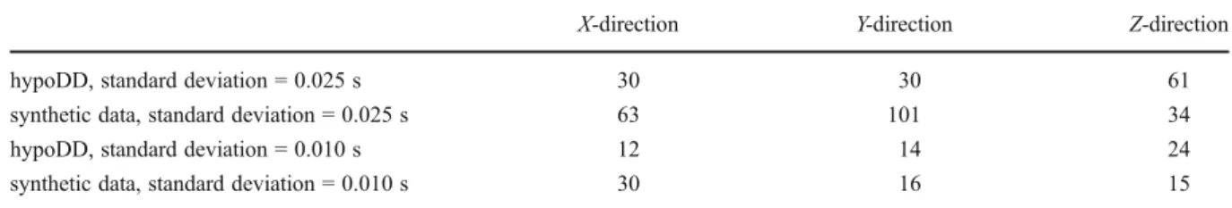
separated. Our results also show nicely the influence of the network geometry on the location results. For both tests, one event shows a slightly larger shift in focal depth, whereas the scatter in focal depth of the remaining events is small (Fig. 13). This particular event is lacking observations of stations CHAT2 and FUSIO; all other events are observed at all 10 stations of the AlpTransit network. The poorer network geom-etry for this particular event is indicated by a larger uncertainty in focal depth, though. Our results demon-strate that hypoDD systematically underestimates lo-cation uncertainties. Since earthquakes within each cluster share the same true location, uncertainties for these events should overlap, which they do not (Fig.13). We estimated mean location errors by com-puting the mean distance between true hypocenter and relocated hypocenter locations of all earthquakes for each direction (Table3). Location errors are largest in X-direction and smallest in Z-direction. This is in

contrast to mean location errors computed by hypoDD, which are largest in Z-direction. Moreover, mean location errors computed by hypoDD are signif-icantly smaller than our estimates in X- and Y-direction but larger in Z-direction (Table3). The ratio between our estimates and those computed by hypoDD becomes smaller for the dataset with smaller errors (standard deviation00.01 s). We attribute these differ-ences to the fact that location errors computed by hypoDD do not account properly for the joint effect of station geometry and pick uncertainties. This effect becomes stronger if larger pick uncertainties are pres-ent. We, therefore, use the ratio between mean location errors computed by hypoDD and our estimates to scale location errors computed for real data, i.e., ratios of 2.5, 1.1, and 0.6 in X-, Y-, and Z-direction, respective-ly, for hypocenter locations relocated with the refined picks.

Figure14shows epicenter locations of earthquakes of clusters 11 and 12. Earthquakes have been relocated using hypoDD and refined picks. Relocated seismicity

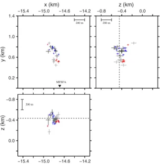
−0.8 −0.4 0.0 −15.4 −15.0 −14.6 −14.2 0.2 0.6 1.0 1.4 y (km) z (km) −15.4 −15.0 −14.6 −14.2 x (km) z (km) −0.8 −0.4 0.0 MFSFA 200 m 200 m 200 m

Fig. 11 Hypocenter locations of earthquakes in cluster 12 using routinely determined P-wave arrival times (gray stars) and adjusted P-wave arrival times (red stars). For the latter, two earthquakes locate at exact the same location, for which reason only seven red stars are seen. Projection of 68% confidence ellipsoid is shown for two earthquakes (marked by small black dot). Hypocenter locations were computed using calibrated P-wave velocities shown in Fig.5. Location of station MFSFA in the Gotthard Base Tunnel is marked by black triangle. Dashed lines mark elevation of the Gotthard Base Tunnel. Map view and two vertical cross-sections along X- and Y-axis are shown. Note that the improved clustering of hypocenter locations if adjusted P-wave arrival times are used

−0.8 −0.4 0.0 −15.4 −15.0 −14.6 −14.2 0.2 0.6 1.0 1.4 y (km) z (km) −15.4 −15.0 −14.6 −14.2 x (km) z (km) −0.8 −0.4 0.0 MFSFA 200 m 200 m 200 m

Fig. 12 Double-difference hypocenter locations of earthquakes in cluster 11 (blue and black crosses) and cluster 12 (red and gray crosses). Same layout as Fig.11. Black and gray crosses mark hypocenter locations obtained using routinely determined P-wave arrival times; blue and red crosses mark hypocenter locations obtained using adjusted P-wave arrival times. Size of the crosses is scaled by error as computed by hypoDD. Dashed lines mark elevation of the Gotthard Base Tunnel. Note that the improved clustering of hypocenter locations if adjusted P-wave arrival times are used

shows a NW–SE striking structure consisting of sev-eral sub-clusters. Location uncertainties for the differ-ent sub-clusters do not overlap suggesting that they occurred at different locations. This is confirmed by a visual check of waveforms recorded at station

MFSFA, located at about 400 m distance from the seismicity (Fig.14). Waveforms of earthquakes within each sub-cluster are nearly identical with similar S–P travel times. Waveforms between the different sub-clusters are distinctively different with varying S–P

MAP VIEW

routine pick uncertainty (0.025 s)

a) b) distance [km] 0.5 0.8 0.6 0.4 0.2 -0.2 0 0.2 -0.5 -0.5 0.5 0 0 distance [km] A A‘ B B‘

Cross Section: A−A‘

distance [km] -0.2 0 0.2 distance [km] depth [km] 0.8 0.6 0.4 0.2 depth [km] Cross Section: B−B‘

MAP VIEW Cross Section: A−A‘ Cross Section: B−B‘

distance [km] 0.5 0.8 0.6 0.4 0.2 -0.2 0 0.2 -0.5 -0.5 0.5 0 0 distance [km] distance [km] -0.2 0 0.2 distance [km] depth [km] 0.8 0.6 0.4 0.2 depth [km] A A‘ B B‘

refined pick uncertainty (0.010 s) hypoDD synthetic data hypoDD synthetic data hypoDD synthetic data hypoDD synthetic data hypoDD synthetic data hypoDD synthetic data

Fig. 13 Tests with synthetic data to assess location errors of double-difference hypocenter locations. Gaussian distributed errors with 0 mean and standard deviations of a 0.025 and b 0.01 s were added to simulate picking uncertainties of routinely determined and refined arrival times picks, respectively. Map view and two vertical cross-sections along A-A′ and B-B′ are shown. Blue and red crosses mark double-difference hypocenter locations computed using synthetic travel times for clusters 11 and 12, respectively. The real set of observations for clusters 11

and 12 was used to compute synthetic travel times. For each cluster, synthetic hypocenter locations were identical (marked by black crosses). Size of the crosses is scaled by error as computed by hypoDD. Mean location errors as computed by hypoDD and as estimated from relocated synthetic hypocenter locations (Table3) are shown by gray crosses. Note that scatter of relocated synthetic hypocenter locations is larger than the size of the crosses, indicating that computed errors are too small. See text for more details

Table 3 Mean location errors (m) as computed by hypoDD and as estimated from tests with synthetic data

X-direction Y-direction Z-direction

hypoDD, standard deviation0 0.025 s 30 30 61

synthetic data, standard deviation0 0.025 s 63 101 34

hypoDD, standard deviation0 0.010 s 12 14 24

synthetic data, standard deviation0 0.010 s 30 16 15

Standard deviation refers to standard deviation of the Gaussian distribution used to simulate picking uncertainties. See text and Fig.13 on details of the tests

travel times (Fig. 14). The ML 2.4 earthquake of March 25, 2006, forms a single sub-cluster suggesting that it occurred on a single structure or fault patch.

4 Source dimensions

Assuming a circular rupture model, the source radius r0 is inversely proportional to the corner frequency fc (e.g., Madariaga 1976; Gibowicz et al.

1990; Abercrombie1995):

r0¼ kc=fc ð1Þ

where c is the wave speed (α for P-wave velocity and β for S-wave velocity) and k is a proportionality factor depending on the source model and wave type. For the static S-wave source model of Brune (1970) k equals 0.375. In the quasidynamic model of Madariaga (1976) k is dependent on the angle θ, which is the angle between the fault normal and the take-off angle of the P- and S-wave at the source. Assuming a good azimuth-al coverage of fcobservations around the source average k values of 0.31 and 0.21 can be used for P- and S-waves, respectively (Madariaga1976). These average k values were computed assuming a rupture speed of 0.9 c. Source radii computed using the Brune model will be

larger than those computed using the Madariaga model due to a larger k value. Studies in Polish mines showed that source dimensions estimated using the Madariaga model are in good agreement with independent obser-vations (see Gibowicz et al.1990and references there-in). We, therefore, decided to use the Madariaga model to estimate source radii. We will use a k value of 0.21 as corner frequencies were estimated from S-wave spectra and only for earthquakes with a good azimuthal distri-bution of stations (see below).

We use a spectral fitting method to compute corner frequency fc, the signal moment (the frequency-independent far-field amplitude), and a path-dependent t* value (Edwards et al. 2010). The ap-proach involves a combined grid-search for fc and Powell’s minimization for the signal moment and t*. Details on the method can be found in Edwards et al. (2008,2010). The grid search over fcis performed at 10% intervals, starting at the equivalent fcvalue for a 0.001 MPa approximate stress drop increasing to the equivalent fcfor a 100 MPa approximate stress drop. The wide search range prevents any bias in the final results. A common fcis assumed for each earthquake across all recordings. Given a good azimuthal cover-age of observations, this will provide a stable avercover-age consistent with our approach to use a constant k value to relate fcto source radii. The inherent coupling of fc

0.2 0.6 1.0 1.4 −15.4 −15.0 X (km) Y (km) −14.6 −14.2 MFSFA 200 m 2006.03.18 M 0.8 2006.03.22 M 0.9 2006.03.25 M 2.4 2006.11.03 M 1.0 2006.11.06 M 1.6 2007.03.01 M 1.3 2006.12.20 M 0.9 0 _{Time [s]} 0.5 2006.02.11 M 0.8 2006.12.04 M 1.2 2006.03.14 M 0.9 2006.02.11 M 1.3 2006.01.26 M 1.3 0 _{Time [s]} 0.4 2006.03.03 M 0.9

Fig. 14 Double-difference epicenter locations and waveforms for earthquakes in clusters 11 (blue) and 12 (red). Epicenter locations were computed using refined arrival times based on cross-correlation measurements. Size of the crosses is scaled by error as computed by hypoDD and adjusted based on tests with

synthetic data (Table3). Band-passed filtered (1–30 Hz) wave-forms of vertical components are shown for station MFSFA (black triangle). Origin times and magnitudes are indicated. Note that scatter in epicenter locations is supported by differ-ences in waveform similarity

and t* requires a priori knowledge on the attenuation structure to derive meaningful fcand stress drop values (e.g., Allmann and Shearer 2007; Edwards et al.

2008). We compute an average Q factor by plotting t* values over hypocentral distance. For constants β and Q, this will yield a straight line with the slope inversely proportional to Q (Anderson and Hough

1984). We use t* values as estimated by the spectral fitting using only highest quality data (i.e., a signal-to-noise ratio >3.5) without any constrains on Q. This yields an average Q of 815. Using data from the Swiss Digital Seismic Network and the same approach, an average Q of 1,216 has been estimated (Edwards et al.

2011). Our lower Q, which implies higher attenuation, seems reasonable considering that a Q of 1,216 repre-sents an average for entire Switzerland and is mainly influenced by ray paths that sample the entire upper crust. Due to short source–receiver distances in our dataset, rays travel only through the shallow upper crust, which can be expected to have a higher attenuation than the entire upper crust. Using an average Q of 815, we re-ran the spectral fitting method to compute fc values, which were then used to compute source radii.

Data processing and quality control are crucial in the determination of source parameters using spectral fitting methods. This is especially important for small magnitude earthquakes, where the low-frequency spectral amplitudes are dominated by the background noise. Data processing follows, in general, the ap-proach of Edwards et al. (2010) with a few adaptations due to the short source–receiver distances in our data-set. First of all, only data from stations located at the surface where used. Given the short source–receiver distance of a few hundred meters, recordings at sta-tions MFSFA and MFSFB were likely still influenced by the near field. All available waveforms are win-dowed to select parts of the data that are characterized by noise and signal. The signal window starts 0.25 s before the S-pick and continues for 20 s. It is conse-quently adjusted to include 5–75% of the cumulative squared velocity of the record (Raoof et al.1999). The minimum signal window is restricted to 2 s. If not available, S-picks are estimated from available manu-ally derived P-picks using a constant Vp/Vs ratio of 1.73. Rescaling of the window length ensures that the position of the window is relatively insensitive to the quality of the P- and S-picks. The noise window starts at the beginning of the trace and continues over a duration equal to 75% of the travel time of the

P-wave. This ensures that the noise window is as long as possible to correctly characterize the long-period noise and that the noise window is not contaminated by the P-wave arrival. Both signal and noise windows are zero padded to create equal length windows and to obtain the 2n samples needed for the fast Fourier transform (FFT). Before applying the FFT, both windows are demeaned and tapered using multitaper algorithms (Park et al.

1987). All data are then deconvolved with the instru-ment response to obtain true ground velocities. The results of these steps are two-sided Fourier ground ve-locity spectra for noise and signal of each trace. An example of adjusted signal and noise windows and corresponding velocity spectra are shown in Fig.15.

To select only the highest quality data, the noise spectrum is automatically shifted to intersect with the signal spectrum at both the lowest and highest fre-quencies of each spectrum (Edwards et al.2010). Only traces where the ratio between signal and noise spectra (SNR) is greater than a pre-defined threshold over a minimum frequency bandwidth of 3–11 Hz are select-ed. We selected an SNR of 1.5 based on visual inspec-tion of the spectra fit of the source model and on the analysis of signal moment amplitudes. Data with SNR <1.5 did not provide stable spectra fits (Fig.15). Moreover, signal moment amplitudes changed considerably for SNR <1.5, whereas amplitudes remained stable for SNR >1.5. In principle, all three components of a seismometer can be used independent-ly in the spectral fitting. On the other hand, we observed significantly lower S-wave signal moment amplitudes for the vertical components. We attributed this to steep incidence angles due to the short source–receiver dis-tances in our data set, which focuses most of the S-wave energy on the horizontal components. We, therefore, used only the average of both horizontal components in the spectral fitting. Averaging of the horizontal com-ponents is done by calculating the geometrical mean of the frequency spectra of the east and north component. We did not rotate the components into the Ray-coordinate system defined by the L, Q, T components due to inherently large uncertainties in estimating inci-dent angles. We expect that uncertainties introduced by this rotation will outweigh the benefits of computing source spectra with a more appropriate coordinate system.

In total, we could compute corner frequencies, and hence source dimensions, for 53 earthquakes out of 112 earthquakes recorded by the AlpTransit Network.

Corner frequencies range from 3 to 11 Hz, which is in good agreement with observations from mining-induced seismicity (e.g., Gibowicz et al.1990). Source radii, based on the source model of Madariaga (1976) range from 50 to 170 m. The largest event of the series, the ML2.4 earthquake of March 25, 2006, has a source radius of 168 m. Except for one earthquake (the March 22, 2006 ML0.9 event) source dimensions could be computed for all earthquakes in clusters 11 and 12 (Fig.16). The largest uncertainty in estimating corner frequencies comes from the trade-off between corner frequencies and whole-path attenuation (t*), which requires a priori knowledge on the Q model as discussed above. We compute average Q values by plotting t* values against hypocentral distance for three different SNRs (1.5, 2.5, 3.5). The corresponding Q values range between 943 (SNR01.5) and 815 (SNR03.5), which corresponds to a change of roughly 10%. The effect of fixing Q to estimate corner fre-quencies is largest for long-distance observations (>100 km) and rather small for short distances (<50 km). For the largest event of the series, the ML0

2.4 earthquake of March 25, 2006, corner frequencies vary between 4.3 Hz (Q0815) and 3.9 Hz (Q0943). This translates into a change in source radii of roughly 10 m for this event. We expect smaller changes for smaller magnitude events as these are mostly recorded at shorter distances. Given our estimated relative loca-tion errors of 15–30 m (Table3) expected uncertainties in source radii become negligible.

As can be inferred from Fig.16, source dimensions overlap within each cluster, with the exception of the June 12, 2006 ML1.2 earthquakes, which are clearly separated from the other events in cluster 12. This suggests that earthquakes within each cluster ruptured the same fault patch or asperity, possibly with slightly different source mechanisms as indicted by small dif-ferences in the waveforms (Fig.14).

5 Discussion and conclusions

Our results show that the observed seismicity occurred in the immediate vicinity of the tunnel system of the

1 0 1 Relative Velocity 1 0 1 Relative Velocity 0 20 40 Time (s) LUKA1_EHE a) b) P S P S 0.01 0.1 1 10 100 Freq.(Hz) 1E-4 1E-3 1E-2 1E-1 1E0 1E1 0.1 0.01 1 10 100 Freq.(Hz) 1E-4 1E-3 1E-2 1E-1 1E0 1E1 0 20 40 Time (s) TONGO_EHE

Fig. 15 Unfiltered waveforms and modeled spectra of stations a LUKA1 and b TONGO for an ML1.3 earthquake of June 12, 2006. Length of noise and signal windows is marked by blue and red dashed lines, respectively. Arrival time of P- and S-wave is marked by solid blue and red lines, respectively. Fourier velocity spectrum (normalized to a peak spectral velocity of

unity) is shown for noise (blue) and signal (red) window. Dashed black lines mark frequency band over which the ratio between noise and signal spectra is computed. Solid black line shows modeled spectra. Note that fit of the modeled spectra is poor for station TONGO due to a low ratio between signal and noise spectra. See text for details on how spectra is modeled

MFS Faido. High-precision epicenter locations of earthquakes in clusters 11 and 12 locate predominant-ly in the more brittle-behaving Leventina gneiss, at a distance of 200–300 m to the northeast of the mapped fault zone (Fig. 17). Source dimensions for these earthquakes outlined two fault patches that ruptured repeatedly during the entire earthquake sequence (Fig.14). The focal mechanism of the ML2.4 March 25, 2006, earthquake, which is part of the largest cluster 11, shows predominantly normal faulting along a NW–SE trending and steeply dipping fault plane (Figs. 9 and 17). Although fault plane solutions for other earthquakes could not be computed, the high degree of waveform similarity indicates that other earthquakes of clusters 11 had similar rupture planes. Orientation of these rupture planes is consistent with strike and dip of the mapped fault zone in the MFS Faido. All this is consistent with a model in which earthquakes occurred predominantly in the more brittle-deforming Leventina gneiss on rupture planes that are associated with a fault system paralleling the mapped fault zone. The same rupture planes were repeatedly activated during the earthquake sequence.

The proximity of the observed seismicity to the tunnel system of the MFS Faido and its close temporal correlation with the ongoing excavation work clearly suggest a causal relationship between the two. In order to understand the stress re-distribution in the vicinity of the MFS Faido due to the excavation, a two-dimensional discontinuum modeling study was per-formed (Hagedorn and Stadelmann 2010). In that study, local geology of the MFS Faido was repre-sented by deformable blocks with their rheological properties estimated from rock samples. Overburden (approx. 1,500 m), rock mass density, and gravity defined an initial vertical stress state of 42 MPa at the top of the model. No horizontal stresses were applied. The modeling results indicated a significant increase in vertical stresses of 20 MPa in the brittle-behaving Leventina gneiss to the east of the fault zone (Hagedorn and Stadelmann 2010). This stress re-distribution was a consequence of the unfavorable combination of overburden, local geology (contact between more brittle and more ductile deforming gneisses), and the existence of a zone of weakness (fault zone). Moreover, horizontal stresses in the Lev-entina gneiss NE of MFS Faido are reduced as a consequence of the significant deformation (shrink-ing) of the excavated tunnel. We propose this increase in differential stress lead to re-activation and con-sequent failure of certain fault segments of the pre-existing fault system (Fig. 18). The fact that fault segments ruptured repeatedly indicates that differential stresses were not entirely released during one event and that ongoing excavation work repeat-edly increased differential stresses. Once excavation work was finished in October 2006 (Fig. 8); differ-ential stresses decayed slowly and seismicity stopped 6 months later.

We successfully recorded and located a series of earthquakes that were induced by the excavation of the tunnel system of the MFS Faido. An accurate knowl-edge of local P-wave velocities, in combination with the density of the seismic network, proved crucial to obtain accurate hypocenter locations. Without this knowledge, focal depths were systematically too deep, even when a regional 3-D P-wave velocity model and S-wave arrivals were used. It is obvious that an inter-pretation based on these wrong focal depths would have come to different conclusions. The proximity of earthquakes to potential triggering sources is still an important criterion to distinguish between natural and

200 m −0.8 −0.4 0.0 −15.4 −15.0 −14.6 −14.2 0.2 0.6 1.0 1.4 y (km) z (km) −15.4 −15.0 −14.6 −14.2 x (km) z (km) −0.8 −0.4 0.0 MFSFA

Fig. 16 Source dimensions of earthquakes in clusters 11 (blue) and 12 (red). Size of the circles is scaled by source dimension as indicated. Black crosses mark corresponding double-difference locations. Source dimensions were derived from corner frequen-cies using source model of Madariaga (1976). Map view and two vertical cross-sections along X- and Y-axis are shown. Note that source dimensions within each cluster overlap suggesting that the same fault patch ruptured repeatedly

induced or triggered seismicity. Hence, the use of accu-rate velocity models for earthquake location remains critical. Our results demonstrate that accurate velocity models can be best estimated from calibration shots.

Great care in interpreting focal depths is needed for studies, in which calibration shots are not available.

Focal depths of the observed seismicity were shal-low, 1–1.5 km below the Earth’s surface. Moreover,

? ? ?

N

?

?

(mapped) Lucomagno gneiss

Leventina gneiss

N

Fig. 17 Epicenter locations of earthquakes in clusters 11 (blue crosses) and 12 (red crosses) in the northern part of the MFS Faido. Epicenter locations were relocated using hypoDD and refined arrival times based on cross-correlation measurements. Size of the crosses is scaled by mean location error as estimated from tests with synthetic data (Table3). Fault plane solution of the ML2.4 earthquake of March 25, 2006 is shown as

equal-area, lower-hemisphere projection. Note that projection has been rotated (57° counter-clockwise) to match north direction. Solid white lines mark mapped faults; dashed white lines mark faults as inferred from fault plane solution and epicenter locations. Local geology and tunnel layout are shown as in Fig.2. Note that earthquakes occurred predominantly in the Levetina gneiss

Leventina gneiss (brittle)

a) prior to excavation b) during excavation

pre-existing fault system Leventina gneiss (brittle) Lucomagno gneiss (ductile) Lucomagno gneiss (ductile) pre-existing fault system re-activated fault segment vertical stress horizontal stress vertical stress horizontal stress excavated tunnel

Fig. 18 Schematic fault model for MFS Faido. a Prior to excavation, a steeply dipping fault zone exist. Existent (hypo-thetical) vertical and horizontal stresses are indicated by white arrows. Planned diameter of tunnel is shown by dashed circles. b During excavation, horizontal stresses are decreased due to

deformation (shrinking) of the tunnel and vertical stresses are increased due to stress transfer by the excavation work. The resulting increase in differential stress leads to failure along a segment of the existing fault system (shown in red). See text for further details

the ML2.4 March 25, 2006, earthquake was strongly felt in nearby villages, likely due to its shallow focal depth. This demonstrates that earthquakes can happen at shallow depth and that they can pose a certain hazard to the general public. As demonstrated in this study, dense seismic networks are important to moni-tor and analyze induced seismicity.

Acknowledgments We wish to thank AlpTransit Gotthard AG for financial support of installation and maintenance of the AlpTransit network. We further wish to thank S. Metzger and B. Baitsch-Ghiradello for their help in the fieldwork and data analysis, and the staff of the Swiss Seismological Service for maintenance and operation of the AlpTransit network. Comments and suggestions from two anonymous reviewers significantly improved the manuscript. This work benefited from fruitful dis-cussion within the AG Mikrobeben consisting of the following members: M. Rehbock-Sander, R. Stadelmann, H. Hagedorn, T. Eppler (all Amberg Engineering AG), D. Kressig, F. Pochop (all AlpTransit Gotthard AG), H.-J. Ziegler (Kellerhals + Haefeli AG), P. Zwicky (Basler & Hofmann).

References

Abercrombie RE (1995) Earthquake source scaling relationships from -1 to 5 M(L) using seismograms recorded at 2.5-km depth. J Geophys Res 100(B12):24015–24036

Allmann BP, Shearer PM (2007) Spatial and temporal stress drop variations in small earthquakes near Parkfield, California. J Geophys Res 112(B4). doi:10.1029/2006JB004395 Anderson JG, Hough SE (1984) A model for the shape of the

Fourier amplitude spectrum of acceleration at high-frequencies. Bull Seismol Soc Am 74(5):1969–1993 Baer M, Deichmann N, Braunmiller J, Husen S, Fah D, Giardini

D, Kastli P, Kradolfer U, Wiemer S (2005) Earthquakes in Switzerland and surrounding regions during 2004. Eclogae Geol Helv 98(3):407–418

Brune JN (1970) Tectonic stress and spectra of seismic shear waves from earthquakes. J Geophys Res 75(26):4997–5009 Diehl T, Kissling E, Husen S, Aldersons F (2009) Consistent phase picking for regional tomography models: application to the greater Alpine region. Geophys J Int 176(2):542– 554. doi:10.1111/J.1365-246x.2008.03985.X

Edwards B, Allmann B, Fah D, Clinton J (2010) Automatic computation of moment magnitudes for small earthquakes and the scaling of local to moment magnitude. Geophys J Int 183(1):407–420. doi:10.1111/j.1365-246X.2010.04743.x Edwards B, Fah D, Giardini D (2011) Attenuation of seismic

shear wave energy in Switzerland. Geophys J Int 185 (2):967–984. doi:10.1111/j.1365-246X.2011.04987.x Edwards B, Rietbrock A, Bommer JJ, Baptie B (2008) The

acqui-sition of source, path, and site effects from microearthquake recordings using Q tomography: application to the United

Kingdom. Bull Seismol Soc Am 98(4):1915–1935.

doi:10.1785/0120070127

Gibowicz SJ, Harjes HP, Schafer M (1990) Source parameters of seismic events at Heinrich Robert mine, Ruhr basin, Federal Republic of Germany: Evidence for nondouble-couple events. Bull Seismol Soc Am 80(1):88–109 Hagedorn H, Stadelmann R (2010) Gotthard Base Tunnel:

UDEC simulations of micro tremors encountered during construction. Analysis of discontinuous deformation: new developments and applications, 373–380. doi:10.3850/ 9789810844554-0016

Husen S, Kissling E, Deichmann N, Wiemer S, Giardini D, Baer M (2003) Probabilistic earthquake location in complex three-dimensional velocity models: application to Switzer-land. J Geophys Res 108(B2). doi:10.1029/2002JB001778 Kradolfer U (1984) Magnitudenkalibrierung von Erdbebensta-tionen in der Schweiz. Diploma Thesis, ETH Zurich, Zurich

Lomax A, Curtis A (2001) Fast, probabilistic earthquake loca-tion in 3D models using Oct-Tree importance sampling. Geophysical Research Abstracts 3

Lomax A, Virieux J, Volant P, Berge-Thierry C (2000) Proba-bilistic earthquake location in 3D and layered models. In: Thurber CH, Rabinowitz N (eds) Advances in seismic event location, vol 18. Kluwer Academic Publishers, Dor-drecht, pp 101–134

Madariaga R (1976) Dynamics of an expanding circular fault. Bull Seismol Soc Am 66(3):639–666

Park J, Lindberg CR, Vernon FL (1987) Multitaper spectral-analysis of high-frequency seismograms. J Geophys Res 92 (B12):12675–12684

Raoof M, Herrmann RB, Malagnini L (1999) Attenuation and excitation of three-component ground motion in southern California. Bull Seismol Soc Am 89(4):888–902 Richards PG, Waldhauser F, Schaff D, Kim WY (2006) The

applicability of modern methods of earthquake location. Pure Appl Geophys 163(2–3):351–372

Rowe CA, Aster RC, Borchers B, Young CJ (2002a) An auto-matic, adaptive algorithm for refining phase picks in large seismic data sets. Bull Seismol Soc Am 92(5):1660–1674 Rowe CA, Aster RC, Phillips WS, Jones RH, Borchers B, Fehler MC (2002b) Using automated, high-precision repicking to improve delineation of microseismic struc-tures at the Soultz geothermal reservoir. Pure Appl Geo-phys 159(1–3):563–596

Rowe CA, Thurber CH, White RA (2004) Dome growth behav-ior at Soufriere Hills Volcano, Montserrat, revealed by relocation of volcanic event swarms, 1995–1996. J Volca-nol Geotherm Res 134(3):199–221

Scherbaum F, Bouin MP (1997) FIR filter effects and nucleation phases. Geophys J Int 130(3):661–668

Tarantola A, Valette B (1982) Inverse problems 0 quest for information. J Geophys 50(3):159–170

Waldhauser F, Ellsworth WL (2000) A double-difference earth-quake location algorithm: method and application to the northern Hayward fault, California. Bull Seismol Soc Am 90(6):1353–1368