One Versus all for deep Neural Network Incertitude (OVNNI) quantification

(1)

HAL Id: hal-03097063

https://hal.archives-ouvertes.fr/hal-03097063

Submitted on 19 Jan 2021

HAL is a multi-disciplinary open access

archive for the deposit and dissemination of

sci-entific research documents, whether they are

pub-lished or not. The documents may come from

teaching and research institutions in France or

abroad, or from public or private research centers.

L’archive ouverte pluridisciplinaire HAL, est

destinée au dépôt et à la diffusion de documents

scientifiques de niveau recherche, publiés ou non,

émanant des établissements d’enseignement et de

recherche français ou étrangers, des laboratoires

publics ou privés.

(OVNNI) quantification

Gianni Franchi, Andrei Bursuc, Emanuel Aldea, Séverine Dubuisson, Isabelle

Bloch

To cite this version:

Gianni Franchi, Andrei Bursuc, Emanuel Aldea, Séverine Dubuisson, Isabelle Bloch. One Versus all

for deep Neural Network Incertitude (OVNNI) quantification. NeurIPS workshop on Bayesian Deep

Learning, Dec 2020, Vancouver, Canada. �hal-03097063�

(2)

One Versus all for deep Neural Network Incertitude

(OVNNI) quantification

Gianni Franchi Andrei Bursuc Emanuel Aldea S´everine Dubuisson Isabelle Bloch

Abstract—Deep neural networks (DNNs) are powerful learning models yet their results are not always reliable. This is due to the fact that modern DNNs are usually uncalibrated and we cannot characterize their epistemic uncertainty. In this work, we propose a new technique to quantify the epistemic uncertainty of data easily. This method consists in mixing the predictions of an ensemble of DNNs trained to classify One class vs All the other classes (OVA) with predictions from a standard DNN trained to perform All vs All (AVA) classification. On the one hand, the adjustment provided by the AVA DNN to the score of the base classifiers allows for a more fine-grained inter-class separation. On the other hand, the two types of classifiers enforce mutually their detection of out-of-distribution (OOD) samples, circumventing entirely the requirement of using such samples during training. Our method achieves state of the art performance in quantifying OOD data across multiple datasets and architectures while requiring little hyper-parameter tuning. Index Terms—Uncertainty estimation, DNN ensembles, one vs all classification, all vs all classification.

I. INTRODUCTION

Deep neural networks (DNNs) have reached state-of-the-art performance on machine learning [34], [17], and computer vision tasks [55], [30]. The significant progress has been leading to their adoption in a wide range of decision making systems, including safety critical ones. Yet, one of the main weaknesses of these techniques appears to be the fact that they tend to be overconfident [18] in their decisions. This issue is difficult to tackle, as the high inner complexity of DNNs results in a poor output explainability.

In order to address this crucial issue, we propose to rely on a finer quantification of the uncertainty of DNN. In contrast to most Bayesian DNN techniques [4], [27], [16], [44], [15], or to frequentist techniques such as Deep Ensembles [32], our approach relies on One vs All (OVA) training. In the statistical learning community, ensembles of OVA or One vs One (OVO) base classifiers for multi-class prediction have been particularly popular in association with Support Vector Machines (SVM), due to SVM being essentially a binary classifier, and to the simplicity of the aggregation rules supported by fundamental theoretical results [28], [31], [60]. The most popular rule in case of OVA ensembles, winner-takes-all (WTA), assigns the testing sample to the class for which the membership score is the highest. For a binary output, the WTA rule creates in the input space multiple unclassifiable regions, for which the class assignment is not unique, and the standard solution is to rely on continuous membership scores. In contrast to SVM-based learning, nowadays the OVA approach has been mostly discarded when training deep classifiers, in favor of All vs All (AVA) learning. MCP scores 0.2 0.4 0.6 0.8 1 confidence score 0 2000 4000 6000 8000 10000 CIFAR10 correct SVHN (OOD) CIFAR10 not correct

(a)

Deep Ensembles scores

0.2 0.4 0.6 0.8 1 confidence score 0 2000 4000 6000 8000 CIFAR10 correct SVHN (OOD) CIFAR10 not correct

(b) OVNNI scores 0 0.5 1 confidence score 0 2000 4000 6000 8000 CIFAR10 correct SVHN (OOD) CIFAR10 not correct

(c)

Fig. 1: Distribution of classifications scores. Here (a), (b) and (c) represent the histograms of confidence scores of Resnet50 [19] trained on the CIFAR10 [29] training set and tested on SVHN [50] and CIFAR10 testing set, using Maximum Class Probability (MCP) [21], Deep Ensembles [32], and OVNNI, respectively. We can see that our proposed algorithm OVNNI outperforms Deep Ensembles (state of the art) and MCP (baseline) on detecting OOD data, since it brings more OOD data to a low score.

Usually, the predictive uncertainty of a DNN is categorized into aleatoric uncertainty and epistemic uncertainty [23]. The former is related to randomness, typically due to the noise in the data. The latter concerns finite size training datasets. The epistemic uncertainty captures the uncertainty in the DNN parameters and their lack of knowledge on the model that generated the training data. In this paper, we propose to use OVA learning in order to improve the quantification of the epistemic uncertainty of the DNN. The underlying idea of our approach is that the score of a base classifier should be adjusted by a factor which approximates its local reliability in the input space from which the test sample originated. Initially for SVM learning, the reliability has been linked to the average value of the local objective function [42], which is approximated using the closest training samples belonging to the respective class. In our algorithm, we propose to adjust the OVA scores by the score provided by an AVA DNN which will play thus the role of approximating the local class-specific objective function. This strategy allows for a particularly effective detection of out-of-distribution (OOD) samples in the testing data, as we can discriminate between samples belonging to unclassifiable regions equally close to some classifiable regions, and samples belonging to unclassifiable regions far from all classifiable regions.

Fig. 1 presents the distribution of the scores provided by the baseline, Deep Ensembles (the current state of the art) and our method, respectively. The baseline is the single AVA classifier, for which the class assignment is performed based on the Maximum Class Probability (MCP). The baseline is unable to discriminate among in- and out-of-distribution

(3)

samples, illustrated in blue/yellow and orange in the histograms, respectively. Deep Ensembles lowers the OOD scores, but the in-distribution membership is still overestimated. Finally, OVNNI successfully assigns low scores to the OOD samples, while keeping at the same time the in-distribution scores high. Our main contributions are the following. We propose an efficient non-Bayesian technique for uncertainty quantification in OOD data classification, that reaches state of the art results on calibration and on OOD data detection on a variety of datasets, and on all typical metrics. Secondly, we perform an extensive study in which we compare, for different applications, with the most significant approaches tackling uncertainty estimation, including Deep Ensembles. Lastly, our conclusions are in line with those of other works which defend the interest of One versus All classifier aggregation [56], and our results rehabilitate this approach in the novel context of uncertainty estimation for DNN.

II. RELATED WORK

OOD detection is not a novel problem and has been studied before the deep learning revival in various branches of machine learning under slightly different taks: anomaly [40], outlier [7] or novelty detection [58]. In the last few years, this task has seen increased attention from different communities and has been addressed with: predictive uncertainty estimation, ensemble methods, image reconstruction, etc. In the following we review briefly some of the methods related to our approach.

Classification with a background class. In multiple computer vision tasks, e.g., object detection [55], [41], it is common to use a background class in addition to the known classes to classify. This leads to a better separation of the classification space and a more discriminative classifier. While this seems to be a reasonable and straightforward approach, for OOD detection, it is likely to suffer from negative dataset bias [59] and thus not generalize to other background objects not seen during training. In our approach, we also use a part of the classes as background when training the individual classifiers, however the overlap of their decision boundaries coupled with the AVA model, better distinguishes in- from out-of-distributions samples.

Anomaly detection by reconstruction. Anomalies can be detected by training an autoencoder [11], [2] or generative model [57], [39] on in-distribution data and use the quality of the reconstruction as a proxy OOD, as the autoencoder is unlikely to decode accurately patterns not seen during training. Training such models for accurate and robust reconstruction requires large amounts of data.

Bayesian approaches. Bayesian Neural Networks (BNN) [49] are elegant, intuitive and easy to reason models, that can capture the epistemic uncertainty through the exploitation of the distributions of their weights. In spite of recent progress that make them more tractable [4], they are still limited to small or medium-size networks, while most DNNs usually enclose millions of parameters. Gal and Ghahramani [16] aimed for a method to imitate BNNs. To this end they proposed Monte Carlo Dropout (MC Dropout) to estimate the posterior predictive network distribution by sampling different

subsets of neurons at each forward pass during test time and aggregate their predictions. In computer vision, MC Dropout is the most popular instance of BNNs due to its speed and simplicity. It has been extended to other tasks, e.g., semantic segmentation [25], pose estimation [26]. However, the benefits of Dropout are more limited for convolutional layers, where specific architectural design choices must be made [25], [48]. Recent OOD benchmarks for semantic segmentation [20], [39] show that MC Dropout still induces many false positives. Ensembles. Ensemble methods are prominent techniques for measuring epistemic uncertainty. They have the potential to encapsulate a true diversity in the weights of the compos-ing models, contrarily to the dispersion introduced by MC Dropout [14], which ultimately focuses on a single mode. Lakshminarayan et al. [32] propose training an ensemble of DNNs with different initialization seeds. Vyas et al. [61] train an ensemble of classifiers in a self-supervised way on different subsets of the training data, using the left-out data as OOD. Izmailov et al. [24] collect weight checkpoints from local minima and average them or fit a distribution over them and sample networks [44]. Franchi et al. [15] track weights trajectories across training and compute their distributions, further used for sampling an ensemble of networks. Our approach also exploits ensembles, however each network is specialized on a different classification task. We exploit the complementarity in this ensemble for better OOD predictions. OVA/OVO ensembles. These aggregation techniques are popular for performing multi-label classification based on an ensemble of binary base classifiers. For OVO, instead of the baseline max-voting aggregation strategy, pairwise coupling [63] or ECOC [13] have been widely used, but the quadratically increasing number of base classifiers may limit significantly OVO applicability in the case of large sets of labels. In contrast, OVA fusion uses a linearly increasing number of base classifiers, and relies in most works on a Winner-Takes-All class assignment based on the maximum class response. To the best of our knowledge, these ensembling methods have not been used for estimating the epistemic uncertainty of DNNs. One-vs-all formulations have also been studied in a more recent publication [52] where an ensemble of one-vs-all DNNs is trained, with a new distance-based loss that can encode the distance of a point from the training manifold, maximizing the binary log-likelihood for the positive class and minimizing it for the negative classes. Despite the interesting results on image classification tasks, this approach does not seem scalable for computer vision tasks such as semantic segmentation. Deep OOD detection. A recent line of approaches addresses OOD detection through DNNs specific heuristics. Hendrycks and Gimpel [21] established a standard baseline for OOD detection relying on the Maximum Class Probability from softmax. In [12] a confidence branch is attached to a classifica-tion network, which is trained to predict OOD samples, while ODIN [38] learns a temperature scaling for softmax values and adversarial perturbation to better distinguish OOD data. Lee et al. [37] get a class conditional Gaussian distribution with respect to features that they tune on a dataset with OOD data and in-distribution data. Lambert et al. [33] attenuate uncertainty by training on a large composite dataset leading

(4)

to a more robust DNN. Zendel et al. [64] propose a semantic segmentation dataset for checking the confidence score of DNNs. The authors of [3] train a DNN to predict OOD confidence score. Lee et al. [36] train a GAN along with the classifier to produce near-distribution examples and enforce lower classifier confidence on GAN samples. Malinin and Gales [45] use Dirichlet networks to build a distribution over the prediction distributions for OOD detection. Most of these methods rely on a OOD dataset during training and are likely to specialize on specific anomalies from these data [22]. In contrast, in our approach we do not require OOD examples during training, as we leverage the multiple one-versus-all classifiers.

III. ONEVERSUS ALL FOR DEEPNEURALNETWORK

INCERTITUDE(OVNNI)

This section focuses first on the necessary details on the traditional AVA training of a DNN. Then we describe our approach based on additional OVA training.

A. Notations

• The training/testing sets are denoted respectively by

Dl = (xi, yi)nl

i=1, Dτ = (xi, yi)

nτ

i=1, where xi and yi

with i ∈ {1...nl} or i ∈ {1...nτ} represent respectively

the observed sample and the corresponding label, with

nl and nτ the size of the training and testing sets. xi

are input vectors and yi∈ {0, . . . , nlabel} are class labels.

Unless otherwise specified, xi and yi, i ∈ [1, nl], will

refer to training data.

• X is the random variable associated with observed samples

and Y the one associated with classes.

• The DNN is a function f of the observed data xi with

i ∈ [1, nl] or i ∈ [1, nτ] and vector ω that contains the trainable weights. We call fω(xi) the output of the DNN associated with the weights ω on the data xi.

• L(ω, yi) is the loss function used to measure the

dis-similarity between the output fω(xi) of the DNN and the expected output yi. Different loss functions can be considered according to the type of task. Here we will focus on the cross entropy that will be introduced in the next section.

B. All Versus All training of Deep Neural Networks

For image classification, the goal of a DNN is to map the input data to a probabilistic prediction that we denote

P (Y = y∗| X = xi, ω) with y∗a class label. During training,

an optimization algorithm will improve the weights ω in order to fit as much as possible the output to the ground truth vector of class labels. The loss is expected to measure the similarity between fω(xi) and yi. Classically we use Cross entropy defined on a batch B of size N ∈ N by:

L(ω(t), B) = −1 N N X i=1 L(ω(t), yi) (1) L(ω(t), B) = −1 N N X i=1 log(P (Y = yi| X = xi, ω)) (2)

The minimization of this loss function is usually based on gradient methods. Computing the optimal value of each parameter involves a bin-to-bin measure of similarity, which may lead to overfitting issues.

A solution might be to use One Versus All training. C. From One Versus All (OVA) to OVNNI

The current state of the art on uncertainty estimation is Deep Ensembles [32]. This technique relies on ensembling multiple DNN models trained in parallel in order to optimize the same loss. In contrast to random forests [6], or Bagging[5] the diversity arises from the fact that different embodiments of the same model will converge towards different local optima during training. Conversely, in our approach the diversity is provided by the one-versus-all (OVA) models constructed using different labelings of the training set.

The OVA strategy is conceptually simple, since at its core it involves training a binary classification DNN. One classifier is trained for each class, and prediction is then performed by running the obtained binary classifiers on the testing sample and choosing the prediction with the highest confidence score. Yet, the multiple classifiers involved will learn multiple probabilistic

predictions, denoted by P (Yj = 1 | X = xi, ωj_{) with Yj} _a

binary random variable for each class j. We add a super script

on ωj_{, to inform that 1) weights are different from the ones}

trained to perform the AVA classification that we denote ω, and 2) they are also different from the weights of other classes different of j.

By training one class versus all the other classes, the DNN learns in some sense the out of distribution classes, however with the significant advantage of not relying on explicitly provided OOD data, in contrast to other strategies [53], [46]. In addition to the OVA base classifiers, we also perform an All versus all training that we aggregate with the probabilities of the OVA models in the following way as shown in Figure 2.

Let us denote by Y the discrete random variable, that is taking its value in the list of all classes, and let us denote by

Yj a binary random variable that takes values 0 or 1, with

Yj = 1 meaning that the data belongs to class j. Hence the

OVA DNN of the class j provides P (Yj = 1 | X = xi, ωj),

while the AVA DNN provides P (Y = j | X = xi, ω) for all

j in [1, nlabel]. We consider that the final confidence score for a

data xi to belong to class j is:

pj(xi) = P (Yj= 1 | X = xi, ωj) × P (Y = j | X = xi, ω) (3)

This score is high if AVA and OVA are confident and low in the other case, multiplying OVA and AVA scores also helps to increase the accuracy since AVA has lower accuracy than OVA.

D. Uncertainty with OVNNI

We consider that a measure of confidence must satisfy the following properties: (1) be bounded, (2) exhibit low values for OOD data, (3) have a confidence value that aligned to the accuracy of the algorithm, (4) get more confident if additional training samples are provided. The first point assures that we

(5)

Fig. 2: From AVA and OVA to OVNNI process in the case we deal with a database composed of just three classes.

know what is the maximum and minimum of confidence. The second point is to ensure to detect OOD data, which is crucial since it provides information on the reliability of the DNN on one data. The third point is linked to the calibration [18], which is crucial to rely on the model predictions. The last point concerns the fact that we want to reduce the uncertainty when increasing the dataset.

We use as a measure of confidence for OVNNI the probability max

j∈[1,nlabel]

{pj(xi)}. This measure is bounded by 0 and 1. In the experimental section, we show that it has a state of the art calibration and OOD results.

E. Visualizing OVA and AVA embedding

In this subsection, we perform two experiments to determine the behavior of the representations learned by the DNN with the different techniques. For both experiments we train a simple DNN composed of 3 hidden layers followed by a batch normalization on MNIST dataset [35].

In the first experiment, we have considered as training data only the images with the digits ’0’,’1’ and ’2’ images (the 3 first classes). Then we perform inference on the official test set composed of images with these classes and the OOD images which are composed of other classes. We represent in Figure 3 the softmax of a classical AVA training, a deep ensemble training and the OVNNI training. One can see that in contrast to other techniques, OVNNI results do not necessarily belong to the 2-dimensional simplex. In addition, OVNNI brings the OOD data far away from the simplex vertices which highlights its potential to detect OOD data.

In the second experiment, we performed a classical AVA training, and we also performed the OVA training. Hence for the OVA training, we have 10 DNNs (since the dataset has 10 classes which are the 10 digits).The OOD class is composed of images of the NotMNIST dataset [1]. Hence, we apply the DNNs on this test dataset and on the AVA case, we collect for each data the feature space of the DNN just before the classification of each data. In the OVA case, we collect the same feature space but for the DNN of the predicted class. We reduce the dimension of each of these feature spaces using T-SNE [43] and Principal Component Analysis (PCA) [62] and we plot the results in Figure 4. We can see that in the AVA case the OOD data are in the center of Figure 4 mixed

with the other classes and in the OVA case they are closer to the border whatever the dimensionality reduction algorithm we use. This is crucial because it shows that OVA learns a more interesting descriptor than OVA.

0.4 0.20.0 0.2 0.4 0.6 0.8 1.0 0.4 0.20.0 0.20.4 0.60.8 1.0 0.4 0.2 0.0 0.2 0.4 0.6 0.8 1.0 MCP simplex representation 0 1 2 OOD (a) 0.4 0.2 0.00.2 0.4 0.6 0.8 1.0 0.4 0.20.0 0.20.4 0.60.8 1.0 0.4 0.2 0.0 0.2 0.4 0.6 0.8 1.0

Deep Ensembles simplex representation 0 1 2 OOD (b) 0.4 0.2 0.0 0.2 0.4 0.6 0.8 1.0 0.4 0.2 0.0 0.20.4 0.60.8 1.0 0.4 0.2 0.0 0.2 0.4 0.6 0.8 1.0

OVNNI simplex representation 0 1 2 OOD

(c)

Fig. 3: Results on MNIST - 3 classes experiments. We represent in these figures the softmax prediction outputs obtained by the baselines (a) MCP, (b) Deep Ensemble, and (c) by OVNNI, respectively.

(a) MCP PCA (b) OVNNI PCA (c) MCP t-SNE (d) OVNNI t-SNE

Fig. 4: Results of the MNIST / NotMNIST experiment. We represent the projection on a 2D space of the feature space of the baseline MCP in figures (a) and (c), and of OVNNI in figures(b) and (d). We use PCA [62] and t-SNE [43] as dimensionality reduction algorithm.

IV. EXPERIMENTS

We continue by illustrating the performance of OVNNI for detecting OOD data by conducting five experiments. In the rest of this section we will describe the experimental protocol, followed by the five experiments. We implemented all approaches ourselves and used for all the same learning hyper-parameters per dataset, without particular tuning. Moreover, the number of ensembles is the same for all the techniques, and corresponds to the number of classes.

A. Experimental protocol

The detection of OOD data can be done either by techniques that measure the uncertainty, or by techniques that detect OOD data. We first have compared our OVNNI to three other uncertainty estimation techniques: MC Dropout [16], Deep

Ensembles [32], and TRADI [15]. The major interest of

these techniques comes from the fact that, since they estimate uncertainty, they also estimate the epistemic uncertainty and therefore the OOD data. We also have compared our approach to two other techniques: ODIN [38] and ConfidNET [10] and serve as references in unsupervised techniques for detecting OOD data. As a baseline algorithm, we use the maximum class probability (MCP) with AVA trained DNN. We denote

(6)

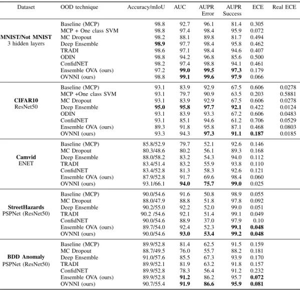
Dataset OOD technique Accuracy/mIoU AUC AUPR AUPR ECE Real ECE Error Success MNIST/Not MNIST 3 hidden layers Baseline (MCP) 98.8 92.7 96.1 81.4 0.305 MCP + One class SVM 98.8 97.4 98.4 95.9 0.072 MC Dropout 98.2 88.1 89.8 81.7 0.494 Deep Ensemble 98.9 97.7 98.4 95.8 0.462 TRADI 98.6 97.1 98.4 94.6 0.407 ODIN 98.8 94.2 96.8 85.6 0.500 ConfidNET 98.2 97.4 98.8 94.1 0.461 Ensemble OVA (ours) 97.2 99.0 99.5 97.3 0.179 OVNNI (ours) 98.8 99.1 99.6 97.9 0.066 CIFAR10 ResNet50 Baseline (MCP) 93.1 83.9 92.9 67.5 0.606 0.0278 MCP +One class SVM 93.1 79.7 90.9 63.5 0.203 0.5881 MC Dropout 93.1 83.9 92.9 67.5 0.606 0.0278 Deep Ensemble 95.0 95.8 97.7 92.1 0.422 0.0124 ODIN 93.1 83.9 93.3 67.2 0.606 0.0483 ConfidNET 93.1 85.1 94.6 61.2 0.706 0.0529 Ensemble OVA (ours) 89.3 91.8 95.8 87.1 0.468 0.0803 OVNNI (ours) 93.3 94.3 97.3 91.1 0.187 0.0185 Camvid ENET Baseline (MCP) 85.8/52.9 79.7 52.1 92.6 0.146 MC Dropout 80.3/48.6 80.2 56.1 89.3 0.168 Deep Ensemble 88.0/58.2 83.2 54.3 94.0 0.112 TRADI 83.4/51.4 83.2 55.9 93.8 0.110 ConfidNET 83.4/52.8 81.3 58.3 92.6 0.121 Ensemble OVA (ours) 87.9/52.8 91.7 69.6 98.4 0.060 OVNNI (ours) 93.1/66.1 94.0 75.7 99.0 0.025 StreetHazards PSPNet (ResNet50) Baseline (MCP) 90.0/54.6 91.6 50.8 98.9 0.055 MC Dropout 88.0/47.9 88.8 51.8 97.8 0.092 Deep Ensemble 90.2/55.0 92.2 52.0 99.0 0.051 TRADI 90.2 /54.6 92.1 51.4 99.1 0.049 ConfidNET 90.0/54.6 88.9 37.0 97.9 0.10 Ensemble OVA (ours) 89.7/54.0 92.4 52.3 99.1 0.048 OVNNI (ours) 90.0/54.6 93.0 53.4 99.2 0.048 BDD Anomaly PSPNet (ResNet50) Baseline (MCP) 89.9/52.8 81.4 62.5 91.5 0.159 MC Dropout 88.7/49.5 76.0 55.7 88.2 0.181 Deep Ensemble 91.0/57.6 85.5 67.3 93.9 0.170 TRADI 89.9/52.1 81.9 63.2 91.8 0.157 ConfidNET 89.9/52.8 78.3 56.4 91.2 0.232 Ensemble OVA (ours) 89.9/52.8 91.2 86.2 95.7 0.072 OVNNI (ours) 90.7/55.4 91.9 86.6 95.9 0.081

TABLE I: Comparative results obtained on the Calibration task.

this approach as MCP. As an additional baseline we consider one-class Support Vector Machine[47], [51], a classic method for outlier detection. We train it on AVA logits.

Note that we have not compared our OVNNI to techniques trained to learn OOD such as [53], [46], since in these case the OOD data are in the training set, making this technique able to detect just with trained OOD data. To balance OVA training which typically has more samples available for the ”All” class, we use weighted cross-entropy to train for each class, with

weights for a given class based on 1 − τclass, where τclass

is the proportion of data samples of this class in the training set. In addition, for a fair comparison in all experiments we use the same number of models for ensemble and Bayesian methods. We conducted several experiments in two target applications: image classification (2 experiments) and semantic pixel segmentation (3 experiments). We considered 7 metrics, in addition to accuracy. Details and results are given below. Metrics. The metric should focus on several points. The first one is the error/success on predicting if the DNN model has some knowledge about specific data. This involves detecting if the data is OOD or not. For that, we use three solutions proposed in [21]. We first only used the confidence score of

the OOD data and on the in distribution test data. Based on these confidence scores, and as in [21], [20], we evaluated the AUC, AUPR and the FPR-95%-TPR, that are indicators of the accuracy of detecting OOD data

However, these measures give no information about the number of good predictions (that should be high) and of bad predictions (that should be low).

This information is crucial since, although it is important to have a low score with the OOD data, the DNN should also reach a high confidence score for well-classified data, and low confidence scores elsewhere. In case the DNN does not reach this point then it might be unusable.

For that, the authors in [10] propose to use metrics similar

to the one used by Hendrycks et al. [21] but rather than

classifying into classes “OOD” or “In distribution”, they classify as “correctly classified” or “not correctly classified” (this latter class contains both bad predictions and predictions on OOD data, see [10] for more details).

We also used the Expected Calibration Error (ECE) [18], which uses the M -bin histograms of confidence scores and accuracy. The ECE performs a bin-to-bin difference between the two histograms, than an average over the M bins. Similarly to [18] we set M = 15. This metric, by measuring the difference

(7)

Dataset OOD technique AUC AUPR FPR-95%-TPR MNIST/Not MNIST 3 hidden layers Baseline (MCP) 94.0 96.0 24.6 MCP + One class SVM 96.9 98.0 12.5 MC Dropout 91.8 94.9 35.6 Deep Ensemble 97.2 98.0 9.2 TRADI 96.7 97.6 11.0 ODIN 94.9 96.7 17.5 ConfidNET 97.9 99.0 12.7

Ensemble OVA (ours) 98.9 99.4 5.9

OVNNI (ours) 99.3 99.6 3.5 CIFAR10 ResNet50 Baseline (MCP) 80.4 89.7 61.5 MCP + One class SVM 78.8 89.6 61.5 MC Dropout 80.4 89.7 62.6 Deep Ensemble 93.0 96.2 19.3 ODIN 80.3 89.9 61.3 ConfidNET 84.8 94.0 68.3

OVNNI (ours) 92.2 95.8 23.3 Camvid ENET Baseline (MCP) 75.4 10.0 65.1 MC Dropout 75.4 10.7 63.2 Deep Ensemble 79.7 13.0 55.3 TRADI 79.3 12.8 57.7 ConfidNET 81.9 13.8 55.8

OVNNI (ours) 96.1 61.2 16.5 StreetHazards PSPNet (ResNet50) Baseline (MCP) 88.7 6.9 26.9 MC Dropout 69.9 6.0 32.0 Deep Ensemble 90.0 7.2 25.4 TRADI 89.2 7.2 25.3 ConfidNET 83.6 2.3 26.2

OVNNI (ours) 91.2 12.6 22.2 BDD Anomaly PSPNet (ResNet50) Baseline (MCP) 86.0 5.4 27.7 MC Dropout 85.2 5.0 29.3 Deep Ensemble 87.0 6.0 25.0 TRADI 86.1 5.6 26.9 ConfidNET 85.4 5.1 29.1

OVNNI (ours) 87.2 6.7 25.0

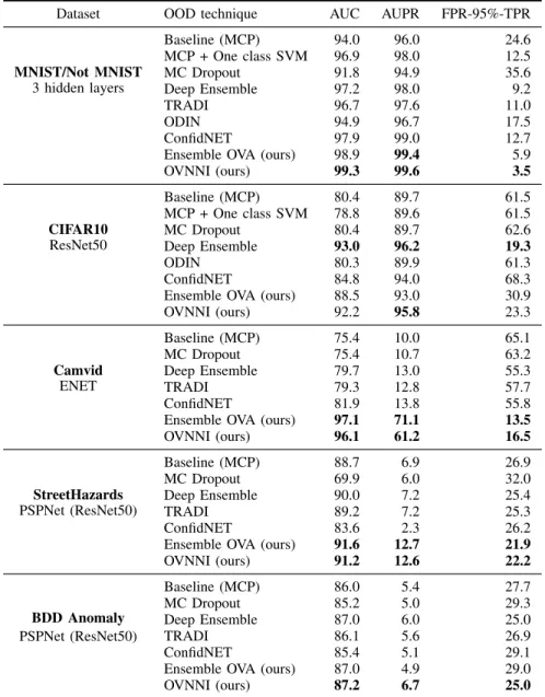
TABLE II: Comparative results obtained on the OOD task.

between the expected accuracy and confidence, is an indicator of the quality of the confidence, and should be close to 0. OOD classification with MNIST [35]. Concerning the classification, we used in a first experiment MNIST [35] which is a dataset composed of digit images as training dataset and NotMnist [1] which contains letter images as OOD dataset. We first trained a classifier to learn to recognize the images of digits then tested it on the test set of MNIST and NotMnist hoping that the classifier would distinguish digits form letters. The DNN used for this experiment is fully connected and composed of 3 layers as in [32], [15]. Results are shown in Tables I and II (MNIST rows).

OOD classification with CIFAR10 [29]. W also trained a network on CIFAR10 composed of classes airplanes, cars, birds, cats, deer, dogs, frogs, horses, ships and trucks. We have considered as OOD SVHN dataset [50]. Many papers [44] train on CIFAR10 and test on the test set of CIFAR10 with noise or on STL-10 [9]. It turns out that the first test aims more at measuring random uncertainty and the second one the

capability to adapt to the domain. We rather have preferred to consider as an OOD dataset SVHN which is a color image dataset of digits, that guarantees that the OOD data really comes from a distribution different from that of CIFAR10. The DNN we used on this experiment is Resnet50 [19], which has the advantage of being popular in the community. Results are shown in Tables I and II (CIFAR10 rows).

OOD Segmentation with Camvid [8]. We used Camvid, a dataset conventionally used in works dealing with segmentation or uncertainty theory and deep learning [25], [10], [15]. This is dataset is an “easy” dataset but allows you to quickly validate results. To test the ability of OVNNI to detect OOD pixels, we trained on all Camvid classes except 3 classes (pedestrian, bicycle, and car), that we deleted, by marking the corresponding pixels as unlabeled. These three classes correspond to OOD classes. Thus this experimental protocol proposed by [15] makes it possible to validate that the trained DNN will detect the pixels on which it has not been trained as OOD. The DNN for this experiment is Enet [54]. Results are shown in Tables I and II (Camvid rows).

(8)

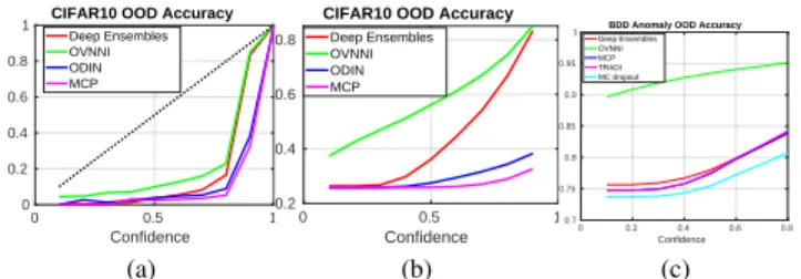
0 0.5 1 Confidence 0 0.2 0.4 0.6 0.8

1 CIFAR10 OOD Accuracy

Deep Ensembles OVNNI ODIN MCP (a) 0 0.5 1 Confidence 0.2 0.4 0.6 0.8

CIFAR10 OOD Accuracy Deep Ensembles OVNNI ODIN MCP (b) 0 0.2 0.4 0.6 0.8 Confidence 0.7 0.75 0.8 0.85 0.9 0.95

1 Deep EnsemblesBDD Anomaly OOD Accuracy OVNNI

MCP TRADI MC dropout

(c)

Fig. 5: (a) and (c) Accuracy vs confidence plot on the CIFAR10 \SVHN and BDD Anomaly experiments, respectively. (b) calibrationn plot on the CIFAR10 \SVHN.

OOD Segmentation with StreetHazards [20]. StreetHazards is a large-scale dataset that contains different sets of synthetic images of street scenes. More precisely, this dataset is composed of 5125 images for training and 1500 test images. The training dataset contains 13 classes and the test dataset is composed of the 13 training classes and 250 OOD classes, making it possible to test the robustness of the algorithms with all possible scenarios. For this experiment we used PSPnet [65] with the experimental protocol in [20]. The architecture used for the PSPnet is ResNet50. Results are shown in Tables I and II (StreetHazards rows).

OOD Segmentation with BDD Anomaly [20]. BDD Anomaly dataset is a subset of BDD dataset, composed of 6688 street scenes for the training set and 361 for the testing set. The training set contains 17 classes, and the test dataset is composed of the 17 training classes and 2 OOD classes. For this experiment we used PSPnet [65] with the experimental protocol in [20]]. The architecture used for the PSPnet is ResNet50. Results are shown in Tables I and II (BDD Anomaly rows).

B. Discussions

On MNIST we can see in Tables I and II that OVNNI has competitive results for detecting OOD data; more specifically, its calibration score (ECE) is the best. With respect to the metrics proposed by Hendryck et al., OVNNI is the most effective in detecting OOD images, improving the best AUC by 1.4% the best AUPR by 0.6% and the best FP of 63.2%. Concerning the metrics proposed by Corbi`ere et al., OVNNI improves the AUC by 1.41%, the AUPR Error by 0.80% the AUPR success by 2.14% and the ECE by 70.6%.

On CIFAR10, although Deep Ensembles achieve good results on all the measurements as well except on the ECE, note that OVNNI is better calibrated. This can also be seen in the histogram in Figure 5. The difference between OVNNI and Deep Ensembles is low and the crucial requirement of DNN is to have a good calibration. Hence, having a good calibration is more important than having a good AUC or AUPR. Also, we have represented the accuracy vs confidence curves in Figure 4. These curves are defined in [32] and are constructed by evaluating the accuracy of all data where the DNN has reached confidence thresholds. These curves show the performance of the OVNNI confidence index over CIFAR10. Finally, we have illustrated the OVNNI calibration on CIFAR10 in the calibration curve in Figure 4. The calibration plot is defined

on [18] and is constructed by taking bins of data based on their confidence score. Then on each bin, we evaluate the accuracy, as it should ideally be comparable to the confidence score. These curves show once again the good performance of OVNNI in terms of calibration.

On Camvid we note that OVNNI improves the results of the state of the art by up to 77% with regard to the metrics proposed by Corbi`ere et al. [10], and by up to 77% for calibration as well. Concerning the metrics proposed by Hendryck et al., OVNNI improves the measurements by a maximum of 22%.

On StreetHazards we show in Table II that OVNNI has better results than the state of the art by improving the best results by up to 42.8%. In Table I OVNNI improves the result by a least 2.6% and improves state-of-the-art ECE by 2%. These results show the interest of using OVNNI for semantic segmentation. Finally, on BDD Anomaly OVNNI improves the calibration by at least 48% which is highly relevant, given the importance of this metric. Furthermore concerning the other metrics, OVNNI improves the results by at least 22%. Furthermore, in Figure 5 we have illustrated the confidence accuracy curve of several algorithms. These curves underline again that OVNNI reaches the best performance in terms of calibration.

Overall, these results show that OVNNI improves the calibration of networks by rendering the confidence in their results more in line with their expected results. Making DNN models more reliable is crucial, especially in areas where the model should not be overconfident. In [18] the authors show that good accuracy of DNNs comes with a price, namely their reliability. In this work, we propose a solution that increases accuracy in most cases, while at the same time improving the calibration and the OOD detection performance. The conceptual simplicity of this solution is a significant asset for its adoption, and the results also convey the message that ’one vs all training’ can still have an interest for a finer understanding of epistemic uncertainty in DNNs.

Ensemble of OVAs and OVNNI act like Deep Ensembles, i.e. discovering and exploring multiple modes [14]. Just like Deep Ensembles, they benefit from the multiple modes provided by each model leading to better calibrated predictions [14]. However, Deep Ensembles can still become overconfident as they follow modern training heuristics [17]. In OVNNI, weighting OVAs with AVA softmax leads to generally less confident predictions and improves calibration (plots in Fig. 5 confirm this quantitatively). This effect is similar to temperature scaling for calibration [17]. However, we do not need an additional validation set to tune this factor. OVA acts as a single class classifier for OOD detection and also learns to perform classification.

V. CONCLUSIONS

In this work, we presented an approach based on One versus all training and mixed with a modern approach based on deep learning. We show that the combination of these approaches reaches states of the art performance on all segmentation experiments. Regarding classification tasks, OVNNI exhibits the best calibration performance. Concurrent approaches suffer from a lack of performance in calibration in most datasets,

(9)

Fig. 6: Results of OVNNI on BDD Anomaly. The first column is the input image, the second is the ground truth, the third is prediction and the fifth is the confidence score of OVNNI. For comparison, we add the MCP confidence score in the fourth column. We can see that OVNNI has a low score on the motorcycle on the three first rows and on the train on the last row which correspond to the OOD classes.

Fig. 7: Results of OVNNI on StreetHazards. The first column is the input image, the second is the ground truth, the third is prediction and the last is the confidence score of OVNNI. For comparison, we add the MCP confidence score in the fourth column. We can see that OVNNI has a low score on the chair, the seat, the rocket and the spider which correspond to the OOD classes.

hence the scores that they provide are overconfident, potentially leading to dangerous scenarios in critical applications. In addition to the reported performance, our approach needs little hyperparameter tuning and is easy to implement.

Future work involves first extending this strategy to new tasks such as medical image analysis. One could also use this framework for active learning since active learning algorithms require techniques that can detect OOD data.

ACKNOWLEDGMENT

This work was supported by ANR Project MOHICANS (ANR-15-CE39-0005). We would like to thank Saclay-IA cluster and CNRS Jean-Zay supercomputer.

REFERENCES

[1] Notmnist dataset. http://yaroslavvb.blogspot.com/2011/09/notmnist-dataset.html [2] Baur, C., Wiestler, B., Albarqouni, S., Navab, N.: Deep autoencoding

models for unsupervised anomaly segmentation in brain mr images. In: International MICCAI Brainlesion Workshop. pp. 161–169. Springer (2018)

[3] Bevandić, P., Kreˇso, I., Orˇsić, M., ˇSegvić, S.: Simultaneous semantic segmentation and outlier detection in presence of domain shift. In: German Conference on Pattern Recognition. pp. 33–47. Springer (2019) [4] Blundell, C., Cornebise, J., Kavukcuoglu, K., Wierstra, D.: Weight uncertainty in neural networks. arXiv preprint arXiv:1505.05424 (2015) [5] Breiman, L.: Bagging predictors. Machine learning 24(2), 123–140 (1996) [6] Breiman, L.: Random forests. Machine learning 45(1), 5–32 (2001) [7] Breunig, M.M., Kriegel, H.P., Ng, R.T., Sander, J.: Lof: identifying

density-based local outliers. In: Proceedings of the 2000 ACM SIGMOD international conference on Management of data. pp. 93–104 (2000)

(10)

[8] Brostow, G.J., Shotton, J., Fauqueur, J., Cipolla, R.: Segmentation and recognition using structure from motion point clouds. In: European conference on computer vision. pp. 44–57. Springer (2008)

[9] Coates, A., Ng, A., Lee, H.: An analysis of single-layer networks in unsupervised feature learning. In: Proceedings of the fourteenth international conference on artificial intelligence and statistics. pp. 215– 223 (2011)

[10] Corbi`ere, C., Thome, N., Bar-Hen, A., Cord, M., P´erez, P.: Addressing failure prediction by learning model confidence. In: Advances in Neural Information Processing Systems. pp. 2898–2909 (2019)

[11] Creusot, C., Munawar, A.: Real-time small obstacle detection on highways using compressive rbm road reconstruction. In: 2015 IEEE Intelligent Vehicles Symposium (IV). pp. 162–167. IEEE (2015)

[12] DeVries, T., Taylor, G.W.: Learning Confidence for Out-of-Distribution Detection in Neural Networks. arXiv e-prints arXiv:1802.04865 (Feb 2018)

[13] Dietterich, T.G., Bakiri, G.: Solving multiclass learning problems via error-correcting output codes. Journal of artificial intelligence research 2, 263–286 (1994)

[14] Fort, S., Hu, H., Lakshminarayanan, B.: Deep ensembles: A loss landscape perspective. arXiv preprint arXiv:1912.02757 (2019) [15] Franchi, G., Bursuc, A., Aldea, E., Dubuisson, S., Bloch, I.: Tradi:

Tracking deep neural network weight distributions. arXiv preprint arXiv:1912.11316 (2019)

[16] Gal, Y., Ghahramani, Z.: Dropout as a bayesian approximation: Repre-senting model uncertainty in deep learning. In: international conference on machine learning. pp. 1050–1059 (2016)

[17] Goodfellow, I., Pouget-Abadie, J., Mirza, M., Xu, B., Warde-Farley, D., Ozair, S., Courville, A., Bengio, Y.: Generative adversarial nets. In: Advances in neural information processing systems. pp. 2672–2680 (2014)

[18] Guo, C., Pleiss, G., Sun, Y., Weinberger, K.Q.: On calibration of modern neural networks. In: Proceedings of the 34th International Conference on Machine Learning-Volume 70. pp. 1321–1330. JMLR. org (2017) [19] He, K., Zhang, X., Ren, S., Sun, J.: Deep residual learning for image

recognition. In: Proceedings of the IEEE conference on computer vision and pattern recognition. pp. 770–778 (2016)

[20] Hendrycks, D., Basart, S., Mazeika, M., Mostajabi, M., Steinhardt, J., Song, D.: A benchmark for anomaly segmentation. arXiv preprint arXiv:1911.11132 (2019)

[21] Hendrycks, D., Gimpel, K.: A baseline for detecting misclassified and out-of-distribution examples in neural networks. arXiv preprint arXiv:1610.02136 (2016)

[22] Hendrycks, D., Mazeika, M., Dietterich, T.: Deep anomaly detection with outlier exposure. arXiv preprint arXiv:1812.04606 (2018) [23] Hora, S. C. (1996). Aleatory and epistemic uncertainty in probability

elicitation with an example from hazardous waste management. Reliability Engineering & System Safety, 54(2-3), 217-223.

[24] Izmailov, P., Podoprikhin, D., Garipov, T., Vetrov, D., Wilson, A.G.: Averaging weights leads to wider optima and better generalization. arXiv preprint arXiv:1803.05407 (2018)

[25] Kendall, A., Badrinarayanan, V., , Cipolla, R.: Bayesian segnet: Model uncertainty in deep convolutional encoder-decoder architectures for scene understanding. arXiv preprint arXiv:1511.02680 (2015)

[26] Kendall, A., Cipolla, R.: Modelling uncertainty in deep learning for camera relocalization. In: Proceedings of the International Conference on Robotics and Automation (ICRA) (2016)

[27] Kendall, A., Gal, Y.: What uncertainties do we need in bayesian deep learning for computer vision? In: Advances in neural information processing systems. pp. 5574–5584 (2017)

[28] Kittler, J., Hatef, M., Duin, R.P., Matas, J.: On combining classifiers. IEEE transactions on pattern analysis and machine intelligence 20(3), 226–239 (1998)

[29] Krizhevsky, A., Hinton, G., et al.: Learning multiple layers of features from tiny images. Tech. rep., Citeseer (2009)

[30] Krizhevsky, A., Sutskever, I., Hinton, G.E.: Imagenet classification with deep convolutional neural networks. In: Advances in neural information processing systems. pp. 1097–1105 (2012)

[31] Kuncheva, L.I.: A theoretical study on six classifier fusion strategies. IEEE Transactions on pattern analysis and machine intelligence 24(2), 281–286 (2002)

[32] Lakshminarayanan, B., Pritzel, A., Blundell, C.: Simple and scalable predictive uncertainty estimation using deep ensembles. In: Advances in Neural Information Processing Systems. pp. 6402–6413 (2017) [33] Lambert, J., Liu, Z., Sener, O., Hays, J., Koltun, V.: Mseg: A composite

dataset for multi-domain semantic segmentation

[34] LeCun, Y., Bengio, Y., Hinton, G.: Deep learning. nature 521(7553), 436–444 (2015)

[35] LeCun, Y., Bottou, L., Bengio, Y., Haffner, P., et al.: Gradient-based learning applied to document recognition. Proceedings of the IEEE 86(11), 2278–2324 (1998)

[36] Lee, K., Lee, H., Lee, K., Shin, J.: Training confidence-calibrated classifiers for detecting out-of-distribution samples. arXiv preprint arXiv:1711.09325 (2017)

[37] Lee, K., Lee, K., Lee, H., Shin, J.: A simple unified framework for detecting out-of-distribution samples and adversarial attacks. In: Advances in Neural Information Processing Systems. pp. 7167–7177 (2018) [38] Liang, S., Li, Y., Srikant, R.: Enhancing the reliability of

out-of-distribution image detection in neural networks. arXiv preprint arXiv:1706.02690 (2017)

[39] Lis, K., Nakka, K., Fua, P., Salzmann, M.: Detecting the unexpected via image resynthesis. In: Proceedings of the IEEE International Conference on Computer Vision (2019)

[40] Liu, F.T., Ting, K.M., Zhou, Z.H.: Isolation forest. In: 2008 Eighth IEEE International Conference on Data Mining. pp. 413–422. IEEE (2008) [41] Liu, W., Anguelov, D., Erhan, D., Szegedy, C., Reed, S., Fu, C.Y., Berg,

A.C.: Ssd: Single shot multibox detector. In: European conference on computer vision. pp. 21–37. Springer (2016)

[42] Liu, Y., Zheng, Y.F.: One-against-all multi-class svm classification using reliability measures. In: Proceedings. 2005 IEEE International Joint Conference on Neural Networks, 2005. vol. 2, pp. 849–854. IEEE (2005) [43] Maaten, L.v.d., Hinton, G.: Visualizing data using t-sne. Journal of

machine learning research 9(Nov), 2579–2605 (2008)

[44] Maddox, W., Garipov, T., Izmailov, P., Vetrov, D., Wilson, A.G.: A simple baseline for bayesian uncertainty in deep learning. arXiv preprint arXiv:1902.02476 (2019)

[45] Malinin, A., Gales, M.: Predictive uncertainty estimation via prior networks. In: Advances in Neural Information Processing Systems. pp. 7047–7058 (2018)

[46] Masana, M., Ruiz, I., Serrat, J., van de Weijer, J., Lopez, A.M.: Metric learning for novelty and anomaly detection. arXiv preprint arXiv:1808.05492 (2018)

[47] Moya, M.M., Hush, D.R.: Network constraints and multi-objective optimization for one-class classification. Neural Networks 9(3), 463– 474 (1996)

[48] Mukhoti, J., Gal, Y.: Evaluating bayesian deep learning meth-ods for semantic segmentation. CoRR abs/1811.12709 (2018), http://arxiv.org/abs/1811.12709

[49] Neal, R.M.: Bayesian Learning for Neural Networks. Springer-Verlag, Berlin, Heidelberg (1996)

[50] Netzer, Y., Wang, T., Coates, A., Bissacco, A., Wu, B., Ng, A.Y.: Reading digits in natural images with unsupervised feature learning (2011) [51] Oliveri, P.: Class-modelling in food analytical chemistry: Development,

sampling, optimisation and validation issues–a tutorial. Analytica chimica acta 982, 9–19 (2017)

[52] Padhy, S., Nado, Z., Ren, J., Liu, J., Snoek, J., & Lakshminarayanan, B. (2020). Revisiting one-vs-all classifiers for predictive uncertainty and out-of-distribution detection in neural networks. arXiv preprint arXiv:2007.05134.

[53] Papadopoulos, A.A., Rajati, M.R., Shaikh, N., Wang, J.: Outlier exposure with confidence control for out-of-distribution detection. arXiv preprint arXiv:1906.03509 (2019)

[54] Paszke, A., Chaurasia, A., Kim, S., Culurciello, E.: Enet: A deep neural network architecture for real-time semantic segmentation. arXiv preprint arXiv:1606.02147 (2016)

[55] Ren, S., He, K., Girshick, R., Sun, J.: Faster r-cnn: Towards real-time object detection with region proposal networks. In: Advances in neural information processing systems. pp. 91–99 (2015)

[56] Rifkin, R., Klautau, A.: In defense of one-vs-all classification. Journal of machine learning research 5(Jan), 101–141 (2004)

[57] Schlegl, T., Seeb¨ock, P., Waldstein, S.M., Schmidt-Erfurth, U., Langs, G.: Unsupervised anomaly detection with generative adversarial networks to guide marker discovery. In: International conference on information processing in medical imaging. pp. 146–157. Springer (2017) [58] Sch¨olkopf, B., Williamson, R.C., Smola, A.J., Shawe-Taylor, J., Platt,

J.C.: Support vector method for novelty detection. In: Advances in neural information processing systems. pp. 582–588 (2000)

[59] Tommasi, T., Patricia, N., Caputo, B., Tuytelaars, T.: A deeper look at dataset bias. In: Domain adaptation in computer vision applications, pp. 37–55. Springer (2017)

[60] Tumer, K., Ghosh, J.: Error correlation and error reduction in ensemble classifiers. Connection science 8(3-4), 385–404 (1996)

(11)

[61] Vyas, A., Jammalamadaka, N., Zhu, X., Das, D., Kaul, B., Willke, T.L.: Out-of-distribution detection using an ensemble of self supervised leave-out classifiers. In: Proceedings of the European Conference on Computer Vision (ECCV). pp. 550–564 (2018)

[62] Wold, S., Esbensen, K., Geladi, P.: Principal component analysis. Chemometrics and intelligent laboratory systems 2(1-3), 37–52 (1987) [63] Wu, T.F., Lin, C.J., Weng, R.C.: Probability estimates for multi-class

classification by pairwise coupling. Journal of Machine Learning Research 5(Aug), 975–1005 (2004)

[64] Zendel, O., Honauer, K., Murschitz, M., Steininger, D., Fernan-dez Dominguez, G.: Wilddash-creating hazard-aware benchmarks. In: Proceedings of the European Conference on Computer Vision (ECCV). pp. 402–416 (2018)

[65] Zhao, H., Shi, J., Qi, X., Wang, X., Jia, J.: Pyramid scene parsing network. In: Proceedings of the IEEE conference on computer vision and pattern recognition. pp. 2881–2890 (2017)

Gianni Franchi received a MSc degree in engineer-ing science from Ecole Centrale Marseille in 2013, and a Ph.D. degree in applied mathematics (2016) from PSL University (Mines ParisTech). Then he did a Postdoc at Siegen University from October 2016 to December 2017. Then he did a Postdoc a Paris Saclay University. He is currently pursuing an assistant Professor at ENSTA Paris. His topics of interest are computer vision, machine learning, statistical learning, video understanding.

Andrei Bursuc is a research scientist at valeo.ai in Paris, France. He completed his PhD at Mines ParisTech in 2012. He was a postdoc researcher at Inria Rennes and Inria Paris. In 2016, he moved to industry to pursue research on autonomous systems. His current research interests concern computer vision and deep learning, in particular learning with limited supervision and predictive uncertainty quantification. Andrei serves regularly as reviewer for major computer vision and machine learning conferences and journals. He is teaching undergraduate courses at Ecole Normale Sup´erieure and Ecole Polytechnique.

Emanuel Aldea is associate professor at Paris-Saclay University. He received his BS and MS degrees in Computer Science from Ecole Polytechnique in 2005 and from Paris 6 University in 2006 respectively, and his PhD in image processing from T´el´ecom ParisTech in 2009. His current research interests include image processing and computer vision for autonomous systems.

S´everine Dubuisson received a Master degree (1997) then Ph.D. degree (2000) in System Control from the University of Technology of Compi`egne. She has been an associate professor in Sorbone Universtity and is currently an associate professor in Aix-Marseille University, France. Her research interests include computer vision, visual tracking, probabilistic models for video sequence analysis and human interaction.

Isabelle Bloch graduated from the Ecole des Mines de Paris, Paris, France, in 1986, and received the master’s degree from the University Paris 12, Paris, in 1987, the Ph.D. degree from the Ecole Nationale Supérieure des Télécommunications (Télécom Paris), Paris, in 1990, and the Habilitation degree from University Paris 5, Paris, in 1995. She has been a Professor at Télécom Paris until 2020 and is now a Professor at Sorbonne Université. Her current research interests include 3-D image understanding, computer vision, mathematical morphology, information fusion, fuzzy set theory, structural, graph-based, and knowledge-based object recognition, spatial reasoning, artificial intelligence, and medical imaging.