HAL Id: hal-02647653
https://hal.inrae.fr/hal-02647653
Submitted on 29 May 2020
HAL is a multi-disciplinary open access
archive for the deposit and dissemination of
sci-entific research documents, whether they are
pub-lished or not. The documents may come from
teaching and research institutions in France or
abroad, or from public or private research centers.
L’archive ouverte pluridisciplinaire HAL, est
destinée au dépôt et à la diffusion de documents
scientifiques de niveau recherche, publiés ou non,
émanant des établissements d’enseignement et de
recherche français ou étrangers, des laboratoires
publics ou privés.
model description and evaluation at 11 eddy-covariance
sites in Europe
Jin Feng Chang, Nicolas Viovy, Nicolas Vuichard, Philippe Ciais, T. Wang,
Anne Cozic, Romain Lardy, Anne-Isabelle Graux, Katja Klumpp, Raphaël
Martin, et al.
To cite this version:
Jin Feng Chang, Nicolas Viovy, Nicolas Vuichard, Philippe Ciais, T. Wang, et al.. Incorporating
grassland management in ORCHIDEE: model description and evaluation at 11 eddy-covariance sites
in Europe. Geoscientific Model Development, European Geosciences Union, 2013, 6 (6), pp.2165-2181.
�10.5194/gmd-6-2165-2013�. �hal-02647653�
www.geosci-model-dev.net/6/2165/2013/ doi:10.5194/gmd-6-2165-2013
© Author(s) 2013. CC Attribution 3.0 License.
Geoscientific
Model Development
Incorporating grassland management in ORCHIDEE: model
description and evaluation at 11 eddy-covariance sites in Europe
J. F. Chang1, N. Viovy1, N. Vuichard1, P. Ciais1, T. Wang1, A. Cozic1, R. Lardy2, A.-I. Graux2, K. Klumpp2,
R. Martin2, and J.-F. Soussana2
1Laboratoire des Sciences du Climat et de l’Environnement, UMR8212, CEA-CNRS-UVSQ,
91191 Gif-sur-Yvette, France
2Grassland Ecosystem Research Unit, French National Institute for Agricultural Research (INRA),
63100 Clermont-Ferrand, France
Correspondence to: J. F. Chang (jinfeng.chang@lsce.ipsl.fr)
Received: 21 March 2013 – Published in Geosci. Model Dev. Discuss.: 8 May 2013
Revised: 20 November 2013 – Accepted: 26 November 2013 – Published: 20 December 2013
Abstract. This study describes how management of
grass-lands is included in the Organizing Carbon and Hydrology in Dynamic Ecosystems (ORCHIDEE) process-based ecosys-tem model designed for large-scale applications, and how management affects modeled grassland–atmosphere CO2
fluxes. The new model, ORCHIDEE-GM (grassland man-agement) is enabled with a management module inspired from a grassland model (PaSim, version 5.0), with two grass-land management practices being considered, cutting and grazing. The evaluation of the results from ORCHIDEE com-pared with those of ORCHIDEE-GM at 11 European sites, equipped with eddy covariance and biometric measurements, shows that ORCHIDEE-GM can realistically capture the cut-induced seasonal variation in biometric variables (LAI: leaf area index; AGB: aboveground biomass) and in CO2
fluxes (GPP: gross primary productivity; TER: total ecosys-tem respiration; and NEE: net ecosysecosys-tem exchange). How-ever, improvements at grazing sites are only marginal in ORCHIDEE-GM due to the difficulty in accounting for con-tinuous grazing disturbance and its induced complex animal– vegetation interactions. Both NEE and GPP on monthly to annual timescales can be better simulated in ORCHIDEE-GM than in ORCHIDEE without management. For annual CO2 fluxes, the NEE bias and RMSE (root mean square
error) in ORCHIDEE-GM are reduced by 53 % and 20 %, respectively, compared to ORCHIDEE. ORCHIDEE-GM is capable of modeling the net carbon balance (NBP) of man-aged temperate grasslands (37 ± 30 gC m−2yr−1(P < 0.01) over the 11 sites) because the management module contains
provisions to simulate the carbon fluxes of forage yield, herbage consumption, animal respiration and methane emis-sions.
1 Introduction
Grassland is a widespread vegetation type, which covers 20 to 40 percent (26.8 to 56 million km2) of the whole land sur-face on the earth, depending on the grassland definition (Sut-tie et al., 2005), and plays a significant role in the global carbon (C) cycle. At the global scale, grasslands were esti-mated to be a net C sink of about 0.5 PgC per year (Scurlock and Hall, 1998), but with considerable uncertainty. Schulze et al. (2009) recently inferred a net C sink in European grass-lands of 57 ± 34 gC m−2yr−1 from a small sample of flux tower net ecosystem exchange (NEE) measurements, com-pleted by C imports/exports at each site to estimate net biome production (NBP). When accounting for emissions of non-CO2greenhouse gases (GHGs) such as methane (CH4)from
grazing animals and nitrous oxide from soil nitrogen (N) ni-trification/denitrification processes, the European grasslands were estimated to be nearly neutral for their radiative forcing, with a net balance of −14±18 g CO2-C eq m−2y−1(Schulze
et al., 2010). Grasslands sequester C in soils – and sequestra-tion is likely favored by high belowground C allocasequestra-tion and root turnover, and possibly by N fertilization (Schulze et al., 2010).
Most of grasslands are cultivated to feed animals, either directly by grazing or indirectly by grass harvest (cutting). Grassland management (including cutting, grazing and fertil-ization) affects the ecosystem C, water and nutrient cycles, as well as the planetary surface energy balance (Feddema et al., 2005; Foley et al., 2005). A net sequestration of C in grass-land soils can be caused by increased litter input associated with increased forage production (Conant et al., 2001) and/or by decreased soil organic matter decomposition, for instance in response to N additions (Berg and Matzner, 1997). Soil C was observed to increase in a grazed semiarid mixed-grass rangeland (Schuman et al., 1999; Reeder and Schuman, 2002) because of an accelerated shoot turnover. However, soil C can also decrease in response to over grazing or poor pasture management (Fearnside and Barbosa, 1998; Abril and Bucher, 1999). Light-to-moderate stocking density was also found to increase C sequestration in the soil (LeCain et al., 2002; Reeder and Schuman, 2002), which was partly attributed to a more diverse plant community and a denser rooting system. Cut grasslands can also sequester C (Sous-sana et al., 2007), but cut European grasslands were on aver-age found to accumulate less C than grazed ones (Soussana et al., 2010). Fertilizer application also affects grassland soil C (Jones and Donnelly, 2004). In particular, a moderate N fertilization was found to increase the organic matter input to the soil more than the soil C mineralization, which favors C sequestration (Soussana et al., 2004).
A better understanding of the C fluxes from grassland ecosystems in response to climate and management requires not only field experiments but also the aid of simulation models. The latter aim at explicitly representing the ac-tual systems, providing a feasible way to predict long-term (compared to experiments) response of ecosystem to exter-nal factors such as climate change and management pro-cesses. Many grassland models have been developed and ap-plied at different scales (from the plot to the global scale). Parton et al. (1988) developed the Century model to sim-ulate soil C, N, P, and S dynamics. The grassland ecosys-tem model (GEM, Hunt et al., 1991; latest version GEM-2, Chen et al., 1996) links biochemical, biophysical and ecosys-tem processes in a hierarchical approach to simulate C and N cycles, but focused only on natural grasslands. A sink-source growth model for prediction of biomass productivity of Lolium perenne grasslands named Lingra (LINtul GRAss) (Schapendonk et al., 1998; Rodriguez et al., 1999) takes cut practice into account. The Simulation of Production and Uti-lization of Rangelands (SPUR2.4, Foy et al., 1999) model is able to track C, N, and water flows in rangeland ecosystems and predicts their response to grazing practice. The Hurley Pasture Model (HPM, Thornley, 1998) describes the C, N and water fluxes in a grazed soil–pasture–atmosphere sys-tem. The process-based model PaSim (Pasture Simulation Model; Riedo et al., 1998) was derived from the HPM to simulate C fluxes exchanged with vegetation, soil and ani-mals and the atmosphere, N2O emissions from soils (Schmid
et al., 2001a, b), NH3 volatilization (Riedo et al., 2002) as
well as CH4emissions from animals (Vuichard et al., 2007a),
considering a range of management options (N fertilization, cutting and grazing practices).
Similarly to plot-scale grassland models, dynamic global vegetation models (DGVMs) are based on equations describ-ing biogeochemical and biophysical processes and simulate the C, N, water and energy fluxes and pools dynamics. These models are generic enough to be applied for regional budgets and long-term simulations, and some of them can be cou-pled with regional or global climate models. Most of them describe vegetation into few plant functional types (PFTs) (i.e., grassland, crop, forest types, etc.) that share the same set of equations and parameters. These models commonly treat grasslands as being unmanaged, thereby ignoring pro-cesses related to agriculture. Only very few DGVMs consider cultivated grasslands, and with simplifications. For example, the LPJmL model (Bondeau et al., 2007) includes an ide-alized “human” or “livestock” disturbance to grasslands by prescribing a removal of 50 % of aboveground grass biomass (AGB) when grazing, with 5 % of grazed AGB entering the litter pool and the rest (95 % of grazed AGB) returning as CO2flux to the atmosphere.
Currently, most of the land surface models have a poor (or no) representation of the management impact on grasslands. Incorporating the grassland management into the Organiz-ing Carbon and Hydrology in Dynamic Ecosystems (OR-CHIDEE) land surface model can improve the model abil-ity in estimating C balance for cultivated grasslands, which enables us to go a step further in assessing C dynamics at-tributed to climate change and human cultivation.
Here, in order to model the impacts of cultivation on Eu-ropean grasslands, we include parameters and functions re-lated to management (e.g., harvested biomass, enteric CH4
emissions and animal production) in the model ORCHIDEE DGVM. The objective of this study is to improve the rep-resentation of grassland by integrating interactions between climate, grass growth and management originating from a managed grassland ecosystem model (i.e., PaSim, Vuichard et al., 2007a) (Sect. 2). Model performance of the modified model was evaluated for 11 eddy-covariance (EC) sites in Europe (Sect. 3) simulating the biometric variables and the monthly to interannual variability of C fluxes.
2 Model description
2.1 ORCHIDEE (Organizing Carbon and Hydrology In
Dynamic EcosystEms)
ORCHIDEE is a process-driven dynamic global vegetation model (DGVM) designed to simulate C and water cycle from site-level to global scale (Krinner et al., 2005; Ciais et al., 2005; Piao et al., 2007). It is composed of two main modules. The SECHIBA (soil–vegetation system and the atmosphere)
parameterization computes the energy and hydrology budget on a half-hourly basis, together with photosynthesis based on enzyme kinetics (Viovy and de Noblet, 1997). These re-sults are fed into a module of ORCHIDEE called STOM-ATE, which simulates C dynamics on a daily basis: gross primary production (GPP) is allocated to different organs, and then respired by the plant or by soil microorganisms when parts of the plant die. These processes determine sev-eral ecosystem state variables such as leaf area index (LAI) and canopy roughness, which are fed back into SECHIBA because they control the energy and water budgets. The equa-tions of ORCHIDEE are described in Ducoudré et al. (1993) for SECHIBA and in Krinner et al. (2005) for STOMATE, and can be found at http://orchidee.ipsl.jussieu.fr/. As in most DGVMs, the vegetation is discretized into a discrete number (13) of PFTs over the globe. For grassland, C3 and C4 grass are included and treated like unmanaged natural systems, where C–water fluxes are only subject to atmospheric CO2
and climate changes. Here we use version 1.9.6, which can be accessed at http://forge.ipsl.jussieu.fr/orchidee/browser/tags/ ORCHIDEE_1_9_6/. The N cycle is not included in this ver-sion of ORCHIDEE.
2.2 PaSim (Pasture Simulation Model)
2.2.1 General structure
PaSim is a plot-scale process-based grassland model devel-oped by Riedo et al. (1998), which simulates grassland pro-cesses at a sub-daily time step. It considers a soil–vegetation– animal–atmosphere system (with state variables expressed per m2)and runs over one to several years. PaSim allows simulating main grassland services such as forage and milk production, as well as the C, N, water and energy fluxes in sown and permanent grasslands. PaSim was applied on a grid to make simulations of grasslands GHG fluxes at the Euro-pean scale by Vuichard et al. (2007b) and was used to run an ensemble of climate change impacts simulations on grass-land services and GHG budgets at French sites (Graux et al., 2012, 2013). PaSim comprises six modules, simulating plant growth, microclimate, soil biology, soil physics, animal pro-cesses, as well as management options. The two latter mod-ules use a daily time step, just as STOMATE does in OR-CHIDEE. See Graux et al. (2012, 2013) for further details about the modelling of grassland processes.
2.2.2 Management simulation
In PaSim, management includes mineral and/or organic N fertilization, and cutting and grazing, which can either be set by the user or optimized by the model (Riedo et al., 2000; Vuichard et al., 2007a; Graux et al., 2011). At each cut-ting operation, a fraction of the shoot biomass is harvested and exported away from the grassland, and a fixed amount corresponding to the residual shoot dry matter (DM) (e.g.,
0.15 kg DM m−2)is left in field. PaSim assumes that a
cer-tain amount (e.g., 5 %) of the grass harvest is lost as lit-ter. For grazing, the version of the animal module of PaSim (version 4.5) developed by Riedo et al. (2000) was further improved by Vuichard et al. (2007a). Riedo et al. (2000) simulated animal herbage intake, milk production (MP), re-turns, respiration and CH4emissions from pastures grazed by
dairy cows or sheep with simplified equations. Vuichard et al. (2007a) further developed this animal module by includ-ing (i) the detrimental effect of tramplinclud-ing on herbage and (ii) cattle selection among shoot compartments when accounting for the grass availability and digestibility (see also Vuichard, 2005, for detailed equations). In the version of Vuichard et al. (2007a), CH4emissions are modeled following
Pinares-Patiˇno et al. (2007) from an empirical-based linear regression of animal emission with digestible neutral detergent fiber in-take (DNDFI) calibrated for dry and early pregnant suckler cows. Simplifications included constant animal live weight and intake capacity during simulation, a grazed only diet and a milk production calculated from the ratio of net energy re-quirements for lactation to the energy content of milk. In this approach, neither the type of animal production (milk, beef) nor net energy requirements for maintenance and produc-tion affected intake. In addiproduc-tion, animals are removed from the paddock when aboveground plant biomass (BM) is lower than a threshold set at 300 kg DM ha−1. Since then, the an-imal module of PaSim (version 5.0) has been improved to simulate mechanistically the diet intake and performances for different types of cattle (suckler cows with their calves, dairy cows and heifers) in response to elevated tempera-tures and management, as well as feedback to the atmosphere through enteric CH4emissions (Graux et al., 2011).
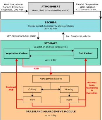
2.3 Coupling strategy
To incorporate into ORCHIDEE a description of manage-ment, our approach is to take the cutting, grazing and fer-tilization options, and the animal module of PaSim (version 5.0, see above) and integrate them into ORCHIDEE. Each day, ORCHIDEE provides AGB to the management mod-ule to be used for cutting or grazing (Fig. 1). Taking into account the types of herbivores (different types of cattle or sheep; Sect. 2.2), the management module simulates har-vested biomass, herbage intake and animal trampling dur-ing grazdur-ing, and followdur-ing C fluxes by animal respiration, milk production, CH4emissions, and excreta returns. Then
it feeds back two variables into ORCHIDEE, the residual AGB fraction, and the newly formed litter. The litter pool of ORCHIDEE is modified from the input of harvested grass residues, manure additions, and from animal trampling ef-fect and excreta returns. We will hereafter refer to the mod-ified version of ORCHIDEE as ORCHIDEE-GM (grassland management). Nine parameters are required for the simula-tions: (i) the timing of cuts and the associated residual total shoot DM (and the residual LAI), (ii) the type of fertilizer, the
Fig. 1. Schematic of ORCHIDEE-GM.
timing of their application and the corresponding amounts, and (iii) the start and length of grazing periods and the graz-ing animals stockgraz-ing rate (nanimal).
2.4 Specific modifications in the ORCHIDEE-GM
As ORCHIDEE is designed to represent the C cycle of un-managed grassland, we adapted the model to include (i) the possibility of reaching high LAI values such as observed in productive managed European grasslands; (ii) the leaf shed in highly dense tillers; (iii) a reduction of the leaf fraction in total AGB, and iv) a translocation of carbon from a reserve pool after cut in order to shape new leaves. In addition, we improved the representation of specific leaf area (SLA) for stimulating regrowth after cutting or grazing. These struc-tural changes made to the ORCHIDEE-GM model code are described below.
2.4.1 LAI limitation in managed grassland and the leaf
shed in highly dense tillers
Formerly, a limitation of LAI (LAImax, 2.5 m2m−2for C3
grass) was prescribed in ORCHIDEE to avoid unrealisti-cally high LAI of unmanaged C3 grass. However, produc-tive grass species selected by agronomists, as well as fer-tilization, make higher LAI possible in grasslands. Accord-ing to maximum LAI observed at 20 European grassland sites (Gilmanov et al., 2007), we alleviated the limitation of
maximum seasonal LAI by increasing the LAImaxparameter
to 7 m2m−2in ORCHIDEE-GM.
Natural grasses in ORCHIDEE seldom shed new leaves during growing season unless “meteorological” leaf senes-cence happens (Krinner et al., 2005). However, highly dense tillers in managed grassland can induce fading of their shaded leaves at the base of the canopy. Thus we added to ORCHIDEE an AGB turnover parameter that depends on tiller density (LAI in the model). For the C pools affected by shading, the rate of loss of their biomass, 1B, is prescribed through
1B = B1t
τ , (1)
where B is the biomass and 1t is the time step of 1 day.
τ (days) is assumed to be a linear function of LAI when a density of grasses (2.5 m2m−2)is reached or surpassed:
τ =max (τmin, τmax−LAI × 10) if LAI > 2.5 m2m−2, (2)
with τmin=45 days and τmax=85 days.
2.4.2 Reduction of leaf fraction in total AGB after
harvest (cut) and following translocation from carbohydrate reserves
During cutting operations, the upper part of AGB is removed, mainly leaves, some stems and all ears. Within the remaining part of AGB near land surface, after cutting, tissues used for sustaining and transporting (stems) become the most signifi-cant proportion of AGB. Thus in ORCHIDEE-GM, we sup-posed a leaf fraction of 10 % and a stem fraction of 90 % in the remaining AGB after a cut event.
Photosynthesis decreases dramatically just after a cut since few leaves remain. A rapid restoration of active photosynthe-sis is thus crucial for plant recovery after defoliation and car-bohydrate reserves play a critical role in sustaining regrowth during the first days after cut (Schnyder and de Visser, 1999). To reproduce this recovery, we placed an additional translo-cation from the ORCHIDEE carbohydrate reserves pool to-ward the leaf biomass pool after each cut, just as it is the case for ORCHIDEE at the leaf onset date, in order to rapidly re-store a relatively dense leaf cover (Krinner et al., 2005).
2.4.3 Age-related SLA
Usually, newly formed leaves have a higher specific leaf area (SLA) value, which decreases with increasing leaf age (Haase et al., 1999; Poorter et al., 2009). Age-related SLA changes were neglected in the standard version of OR-CHIDEE, which has a PFT-specific, fixed SLA value. How-ever, in managed grasslands, the age of leaves is modified by cutting/grazing, and SLA variations with leaf age be-come important. Newly formed leaves with higher SLA help the plant to increase rapidly its LAI with a relatively small
amount of biomass. Therefore we let SLA depend on leaf age class and on the fraction of leaf mass in that class.
There are four leaf age classes in ORCHIDEE. At each time step, GPP allocated to leaves is incorporated into leaf biomass of age class 1, and a fraction of the leaf biomass passes from age class i to age class i +1. This process results in an increasing age of the canopy during the growing period. We calculated SLA as SLA = 4 X i=1 slai×fi, (3)
where fi is the fraction of leaves in age class i, and slai is the prescribed maximum SLA (SLAmax) for age class
i. The value of sla1 equals to SLAmax, then to a fraction
of 0.90, 0.85 and 0.80 of SLAmax for leaf age class 2, 3
and 4, respectively. In ORCHIDEE-GM, SLAmax is set to
0.048 m2g−1C, a value chosen to fit the mean SLA value
of C3 grass in the global TRY database (0.0201 m2g−1DM,
equal to 0.0422 m2g−1C with mean leaf carbon content per dry matter of 47.61 %; Kattge et al., 2011).
3 Evaluation at European grassland sites
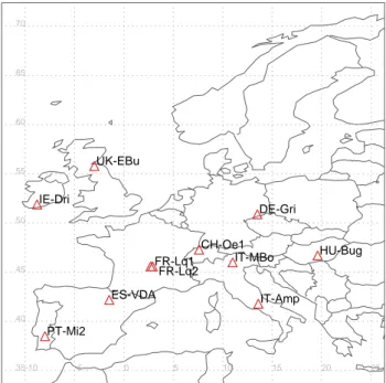
3.1 Site selection and description
To evaluate ORCHIDEE-GM, we ran ORCHIDEE and ORCHIDEE-GM at 11 European grassland sites (Fig. 2) with contrasted management intensity, where good quality flux data (NEE, measurements by eddy-covariance (EC) tech-nique) were collected, the data being gap-filled and parti-tioned to GPP and TER (total ecosystem respiration) us-ing the CarboEurope-IP methodology (see CarboEurope-IP project, e.g., Dolman et al., 2006; Reichstein et al., 2005; Papale et al., 2006; Moffat et al., 2007; Béziat et al., 2009). The 11 sites have sufficiently detailed management records (management type, timing of cutting or grazing, and corre-spondingly harvest severity or stocking density). There are three cut sites, six grazed sites and two mix-managed sites. The geographic information, management type, fertilization practice, year with management or C fluxes records, and mean meteorological variables are listed in Table 1. It should be noted that the enhanced version of the PaSim animal mod-ule (version 5.0) was used in the simulations at FR-Lq1 and FR-Lq2, where animal type (heifers) and characteristics data were available (Graux et al., 2011). At the other grazed sites, due to the lack of such detailed input data on animals, version 4.5 animal module was used instead.
Laqueuille (FR-Lq1 and FR-Lq2) has been a 6.7 ha per-manent grassland for at least 50 yr, grazed by heifers from May to October. The intensively grazed Laqueille site (FR-Lq1, 2.8 ha) is prescribed with a mean stocking density of
∼1 LSU ha−1yr−1and is fertilized with ammonium nitrate in three splits. The extensively grazed site (FR-Lq2, 3.4 ha) is
-10 -5 0 5 10 15 20 25 35 40 45 50 55 60 65 70 CH-Oe1 DE-Gri IT-MBo ES-VDA HU-Bug IE-Dri UK-EBu IT-Amp PT-Mi2 FR-Lq1 FR-Lq2
Fig. 2. Distribution of the 11 European grassland sites in this study.
maintained at half the stocking rate of the intensive paddock and is not fertilized.
Grillenburg (DE-Gri) is a permanent grass-clover mixture managed with 2–4 cuts per year and without fertilization.
Bugac (HU-Bug) is a semi-arid sandy grassland part of the Kiskunság National Park that has been under extensive management (grazing) for the last 20 yr. However, the man-agement data are not known at this site in a protected area.
Dripsey (IE-Dri) is a perennial ryegrass pasture grazed for approximately 8 to 10 months of the year, and fertilized with
∼200 kg N ha−1yr−1.
Amplero (IT-Amp) is a Mediterranean grassland site, char-acterized by summer drought, and is subjected to a once-a-year mowing at the peak of the growing season and some subsequent cattle grazing periods.
Monte Bondone (IT-MBo) is an alpine meadow with pre-cipitation peaking in summer. It is managed with one cut per year in mid-July.
Mitra (PT-Mi2) is composed of C3 annuals, which die-out by the end of spring, and of one invasive C4 grass. The climate is Mediterranean, with a hot and dry summer, and most of the precipitation occurs between October and April. The grassland is highly seasonal. Its growth begins after the autumn rains and lasts until May–June when normally soil water content decreases strongly.
Vall d’Alinya (ES-VDA) subalpine grassland is located in the Mediterranean mountain regions of Spain, characterized by a distinct summer drought. It is moderately cattle-grazed during the summer growing season (0.2–0.4 LSU ha−1).
Oensingen (CH-Oe1) grassland has been sown with grass-clover mixtures in 2001. It is cut four times a year and
Table 1. Location, climate and management for the 11 managed grassland sites in Europe (from the FLUXNET program, http://www.fluxnet.
ornl.gov; Baldocchi et al., 2001).
Altitude MAT MAP Fertilization Year of Year of Site Code Country Latitude Longitude (m) (◦C) (mm yr−1) Management (kgN yr−1) simulation fluxes Laqueuille 1 FR-Lq1 France 45◦380N 02◦440E 1040 7.9 897 Grazing 172–213 2002–2009 2004–2009
Laqueuille 2 FR-Lq2 France 45◦380N 02◦440E 1040 Grazing – 2002–2009 2004–2008
Grillenburg DE-Gri Germany 50◦570N 13◦300E 385 8 439 Cutting – 2004–2008 2004–2008
Bugac HU-Bug Hungary 46◦410N 19◦360E 111 10.6 477 Grazing – 2003–2008 2003–2008 Dripsey IE-Dri Ireland 51◦550N 08◦450W 186 9.6 1271 Grazing ∼200 2003–2005 2004–2005 Amplero IT-Amp Italy 41◦520N 13◦380E 900 10.2 755 Cutting/Grazing – 2003–2007 2003–2006 Monte Bondone IT-MBo Italy 46◦000N 11◦020E 1550 5,1 999 Cutting – 2003–2007 2003–2007
Mitra PT-Mi2 Portugal 38◦320N 08◦000W 190 15,6 550 Cutting/Grazing – 2005–2007 2005–2007
Vall d’Alinya ES-VDA Spain 42◦120N 01◦260W 1770 6.5 891 Grazing – 2004–2008 2004–2008 Oensingen CH-Oe1 Switzerland 47◦170N 07◦440E 450 9.5 1206 Cutting ∼200 2002–2009 2002–2008 Easter Bush UK-EBu United Kingdom 55◦520N 03◦020W 190 9 965 Grazing ∼265 2004–2008 2004–2008
Notes: MAT, mean annual temperature; MAP, mean annual precipitation.
fertilizers are applied as solid ammonium nitrate or liquid cattle manure (∼ 200 kg N ha−1yr−1).
Easter Bush (UK-EBu) grassland is intensively man-aged with cutting for silage (2002–2003) and grazing by dairy cattle and sheep (2004–2008). It receives on average 265 kg N ha−1yr−1 as N-P-K fertilizer. The climate at this site is oceanic with mild winters and cool and moist sum-mers.
3.2 Meteorological data
Meteorological data required as input by ORCHIDEE and ORCHIDEE-GM are half-hourly air temperature, precipi-tation (each event), wind speed, atmospheric water vapor pressure, net radiation, long-wave incoming radiation, mean near-surface atmospheric pressure and annual CO2
atmo-spheric concentration. All the meteorological variables were measured on top of each flux tower on a half-hour time step, meeting the requirement of the models, except for CO2,
which is taken from atmospheric background measurements. The forcing data were firstly cleaned and then gap-filled ac-cording to the methods as follows (see Falge et al., 2001). For small gaps (e.g., one or two hours), linear interpolation was used; for bigger gaps (e.g., one or two days), data from days with similar pattern were adopted; for gaps longer than 10 days (e.g., in winter at cold sites, the data were gap-filled with data from similar previous year; if necessary, precipita-tions have been corrected in order to get the correct total an-nual sum. The long-wave incoming radiation (few measure-ments are available at the sites) and mean near surface atmo-spheric pressure (not measured at the sites) were extracted from the 6-hourly CRU-NCEP 0.5◦×0.5◦ global database (http://www.cru.uea.ac.uk/cru/data/ncep/), which are linear interpolated to half-hourly.
3.3 Models setup
Site-level simulations were conducted with ORCHIDEE and with ORCHIDEE-GM separately. All simulations started from an equilibrium state of C pools with climate and
management obtained with a model spin-up. To initialize ORCHIDEE and ORCHIDEE-GM, we first ran each model without management until all ecosystem C pools reached steady state (spin-up 1); site-specific meteorological data is repeatedly cycled to force each model (Table 1). In real-ity, the equilibrium state of natural ecosystem C pools (after spin-up 1) can be changed by management practices. How-ever, the management history is not clear at the site level. Thus, we assume a general (idealized) management history for each site, i.e., the same management practices as used nowadays have been applied to the additional 40 yr after spin-up 1 to obtain the ecosystem C pools under the grass-land management. Thus, starting from the end of spin-up 1, ORCHIDEE-GM was run for another 40 yr with the same meteorological data and management practices correspond-ing to the (idealized) management history of each site (spin-up 2). Finally, starting from the end of spin-(spin-up 2, simulations were conducted for the target period of evaluation (Table 1).
3.4 Methods for evaluating model performance
To assess model–data agreement for biometric variables such as LAI and AGB, we use the index of agreement (IOA, Willmott et al., 1985; Legates and McCabe, 1999), given by
IOA = 1.0− n X i=1 (Oi−Pi)2/ n X i=1 (|Pi−O|+|Oi−O|)2, (4)
where Piis modeled data, Oiis observed data, O is observed mean, and n is number of data. The index of agreement can overcome the insensitivity of correlation-based measures to differences in the observed and modeled means and variances (Willmott et al., 1985). It varies from 0.0 to 1.0, with higher values indicating better model–data agreement.
Ecosystem–atmosphere fluxes are shaped by a variety of fluctuations on different scales of characteristic variability. Scalar error estimates and residual analysis used to sum-marizing model–data disagreement provide only limited in-sight into the quality of a model (Mahecha et al., 2010). A more sophisticated way could be localizing model–data
Table 2. Limits of the two frequency binning schemes.
Bins Upper Limit p[d] ≤ . . . Lower Limit p[d] > . . . Denotation
A maximum 582.9 low-frequency variability B 582.9 132.2 seasonal-to-annual variability C 132.2 33.1 intermonthly variability D 33.1 minimum daily-to-weekly variability Notes: The discretization is approximately log-equidistant and provides the basis for all multiple timescales CO2fluxes analysis. The choice of the binning is a trade-off, taking into account the requirements for an ecological interpretation and the limitations in the frequency definition of the reconstructed components (in the SSA framework).
mismatches in time (Gulden et al., 2008). Thus, to evaluate time-frequency localized model performance on CO2fluxes
(GPP, TER and NEE), we used a time domain decomposition method called SSA (singular-spectrum analysis; Broomhead and King, 1986; Elsner and Tsonis, 1996; Golyandina et al., 2001; Ghil et al., 2002). Observed and modeled time series can be described as sets of additively superimposed subsig-nals, which can be expressed as
Y =XXi, i =1. . .N, (5) where Xi is the subsignal of corresponding temporal scales. SSA is used to extract subsignals Xi of a given time se-ries. The SSA method was shown to be suitable for ex-ploring the time variability of eddy-covariance ecosystem– atmosphere fluxes (Mahecha et al., 2007), and was used to explore model–data misfit on multiple timescales (Mahecha et al., 2010). In this study, based on the signal decompo-sition and reconstruction from SSA technique (Golyandina et al., 2001; for technical details see Mahecha et al., 2010, Appendix B), the original time series can be separated into four timescale variabilities: daily-to-weekly, intermonthly, seasonal-to-annual, and low-frequency (Table 2). EC obser-vations were not fully available for all the years we simulated (Table 1). Thus, time series with continual full year gap-filled EC observations are used to derive the subsignals (time span for each site are listed in Table 1). The subsignals extracted by the SSA method provide information for a qualitative and quantitative model–data comparison on different timescales (Mahecha et al., 2010).
Model–data agreement of CO2 fluxes for each
SSA-extracted or combined subsignal is assessed with a Pearson’s product–moment correlation coefficient (r) and root mean squared error (RMSE). The Pearson’s product-moment cor-relation coefficient (r) describes the proportion of the total variance in the observed data that can be explained by the model, given by r = n P i=1 (Pi−P )(Oi−O) s n P i=1 (Pi−P )2 s n P i=1 (Oi−O)2 , (6)
where Pi is modeled data, Oiis observed data, P is modeled mean, O is observed mean, and n is the number of data. The root mean squared error (RMSE) is a measure of model ac-curacy reporting the mean difference between the modeled and observed fluxes, expressed as
RMSE = v u u t n X i=1 (Pi−Oi)2/n, (7)
where Pi is modeled data, Oi is observed data, and n is the number of data.
Short time span of observed CO2fluxes reduced reliability
of interannual variability extracted by SSA. Thus, we con-sider an ensemble approach to assess model performance for interannual variability of CO2fluxes, which combines data of
all years at all sites and gives a total of 53 site-years for the analysis. In order to quantify the interannual variability, we normalized observed–modeled CO2fluxes by subtracting the
long-term calendar year observed–modeled mean annual flux for each site-year fluxes. First, biases in model estimates of each CO2flux are identified (observed–modeled) for
calen-dar year average observed–modeled fluxes. Then, r between observed and modeled interannual variability indicates the correlation, and RMSE is used to assess model–data agree-ment on long-term timescale.
3.5 Carbon input/export and NBP calculation
When simulating CO2exchanges in managed grasslands, one
has to take into account animal respiration in the calculation of TER at grazed sites. NEE in ORCHIDEE-GM at grazed sites is calculated as:
NEE = Rhet+Rauto+Ranimal−GPP, (8)
where Rhet, Rautoand Ranimal are heterotrophic, autotrophic
and animal respiration, respectively. Negative value of NEE indicates a net CO2sink.
Besides flowing between plant, soil and atmosphere, C is exported by grass harvest (Charvest)and through animal
prod-ucts formed from grazing (CCH4, Cliveweightand Cmilk); C is also added to the ecosystem by organic fertilizer application (Cfert). For example, slurry or manure is applied at CH-Oe1,
3.8 4.0 4.2 4.4 4.6 4.8 dm 2 gC -1 0 1 2 3 4 m 2 m -2
Jan Mar May Jul Sep Nov JanJan Mar May Jul Sep Nov Jan
SLA
LAI
CUT GRAZE
2007 2007
Fixed SLA Age-related SLA
1027
Figure 3
1028
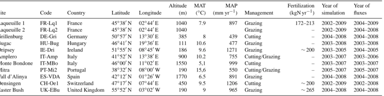
Fig. 3. Age-related SLA and its impact on LAI. Results are
simu-lated by ORCHIDEE-GM with fixed SLA and age-resimu-lated SLA re-spectively on a mowed grassland (CH-Oe1) and a grazed grassland (FR-Lq1) for the year 2007.
respectively). When C input/export is taken into account, the net carbon balance (NBP) of a site can be estimated as NBP = Cfert−Charvest−Cliveweight−Cmilk−CCH4−NEE. (9) Positive value of NBP indicates a net C sink of the ecosys-tem. Animal liveweight gain (Cliveweight) during grazing
comprises only little part of C export (less than 10 % of Cmilk;
see Byrne et al., 2007). In this study, Cliveweight was not
de-termined and will be neglected for the calculation of NBP.
4 Results
4.1 Age-related SLA variation and its effect on LAI
With age-related SLA incorporated in ORCHIDEE-GM, an abrupt rise of SLA at the leaf onset and its subsequent de-crease as canopy ages before the next cutting or grazing event (Fig. 3). After a cutting event, C translocation from carbohy-drate reserves stimulates the formation of new leaves, and then the SLA begins to sharply rise again. For grazing, the SLA does not fluctuate as much as for cutting (Fig. 3), which reflects continuous biomass consumption and leaf regener-ation. Finally, at the end of the growing season, SLA de-creases because of leaf senescence, and a low value is main-tained until the next leaf onset in spring. The average grow-ing season SLA across the 11 sites in ORCHIDEE-GM is of 0.0424 ± 0.0010 m2g−1C, which is close to the observed value of 0.0201 m2g−1DM (equal to 0.0422 m2g−1C, with mean leaf carbon content per dry matter of 47.61 %) reported by Kattge et al. (2011) in the TRY database for 594 species (5033 observations) around the world. The dynamic SLA modeling accelerates grasses regrowth (higher LAI during
0 1 2 3 4 5 6 m 2 m -2 0.0 0.2 0.4 0.6 0.8 1.0 kg DM m -2 -30 3 6 9 12 15 18 g C m -2 day -1 -30 3 6 9 12 15 18 g C m -2 day -1
Apr Jul Oct Jan Apr Jul Oct Jan Apr Jul Oct
-12-9 -6 -3 0 3 6 9 g C m -2 day -1 LAI AGB GPP TER NEE 2005 2006 2007
ORCHIDEE ORCHIDEE-GM OBSERVATION
1029
Figure 4
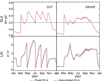
1030 Fig. 4. Comparison of simulated/observed biometric variables and
carbon fluxes for the cut grassland of Oensingen, CH-Oe1. LAI, leaf area index; AGB, aboveground biomass (dry matter); GPP, gross primary production; TER, terrestrial ecosystem respiration; NEE, net ecosystem exchange. GPP, TER and NEE are presented as 15 day running means to smooth out very high frequencies.
growing season in Fig. 3), but the effect on LAI remains small (difference of 2.35 % for annual mean LAI).
4.2 Comparison between simulated and observed LAI,
AGB and CO2fluxes
At the intensively managed sites (cut: CH-Oe1 and grazed: FR-Lq1), LAI, AGB, and CO2fluxes (GPP, TER and NEE)
are compared between the two models, ORCHIDEE and ORCHIDEE-GM, and the observations (Figs. 4 and 5). In ORCHIDEE, as leaf onset is initialized, LAI steadily in-creases to reach its predefined maximum value (2.5 m2m−2),
which is maintained until the senescence occurs. Compared to ORCHIDEE-GM, the seasonal covariance between LAI and AGB could only be found during the periods of plant growth and senescence in ORCHIDEE (Figs. 4 and 5).
At cut site CH-Oe1, the observed LAI, AGB and GPP have dropped abruptly immediately after cutting and restore to a high values within a short time period (e.g., half-month) af-ter cutting (Fig. 4). The same effect is also present in NEE.
0 1 2 3 4 m 2 m -2 0.0 0.2 0.4 0.6 0.8 1.0 kg DM m -2 -30 3 6 9 12 15 18 g C m -2 day -1 -30 3 6 9 12 15 18 g C m -2 day -1
Apr Jul Oct Jan Apr Jul Oct Jan Apr Jul Oct
-12-9 -6 -3 0 3 6 9 g C m -2 day -1 LAI AGB GPP TER NEE 2005 2006 2007
ORCHIDEE ORCHIDEE-GM OBSERVATION
1031
Figure 5
1032 Fig. 5. Comparison of simulated/observed biometric variables and
carbon fluxes for the grazed grassland of Laqueuille, FR-Lq1.
These large saw-teeth like fluctuations between two cuts are better reproduced by ORCHIDEE-GM than ORCHIDEE. However, ORCHIDEE-GM simulates lower TER than the observations (Fig. 4).
For the intensively grazed site FR-Lq1, ORCHIDEE-GM shows a moderate ability to simulate the grazing-induced AGB and LAI limitation (Fig. 5). For example, during the grazing season (May–October) the low and variable AGB and LAI values are partly captured. By contrast, ORCHIDEE without management is unable to reproduce AGB and LAI because it lacks permanent grass consumption and regrowth. ORCHIDEE-GM can simulate the seasonal cycle of NEE better than ORCHIDEE at the FR-Lq1 grazed site. As shown in Fig. 5, both observed and ORCHIDEE-GM modeled NEE switches from a strong sink of atmospheric CO2(largest
neg-ative NEE) in early growing season (e.g., May–June in 2007) to near zero values during the peak growing – grazing season (e.g., June–July in 2007), followed by the resumption of a small CO2sink at the end of the growing season (e.g., July–
August in 2007) because of grazing-stimulated grass uptake of CO2. -5 0 5 10 15 20 g C m -2 d a y -1 -10 -5 0 5 10 g C m -2 d a y -1 -10 -5 0 5 10 g C m -2 d a y -1 -10 -5 0 5 10 g C m -2 d a y -1
May S ep J an May S ep J an May S ep J an May S ep J an May S ep J an May S ep -10 -5 0 5 10 g C m -2 d a y -1 OB S E R V AT ION OR C HIDE E OR C HIDE E -G M S u b si g n a l e xt ra ct io n b y S S A
Original time series
Low frequency variability
Annual-seasonal variablility
Inter-monthly variability
Daily-to-weekly variability
2002 2003 2004 2005 2006 2007
Fig. 6. Model–data comparison on multiple timescales. Observed
and modeled time series are decomposed into subsignals corre-sponding to characteristic frequency bins. Qualitative or quantita-tive model–data comparisons can be carried out on the correspond-ing pairs of subsignals. Figure 6 exemplifies the model–data com-parison with two models simulations of GPP and corresponding ob-servations at the CH-Oe1.
4.3 General performance of ORCHIDEE-GM
4.3.1 Biometric variables
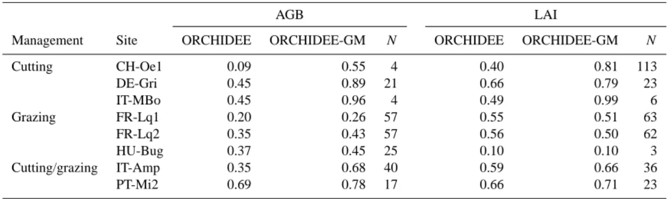
As shown in Table 3, ORCHIDEE-GM has a greater IOA (in-dex of agreement) (AGB: 0.80 ± 0.22 and LAI: 0.86 ± 0.11) than the original ORCHIDEE version (AGB: 0.33±0.21 and LAI: 0.52 ± 0.13) at the 3 cut sites (CH-Oe1, DE-Gri and IT-MBo). At the 3 grazed sites (FR-Lq1, FR-Lq2 and HU-Bug), ORCHIDEE-GM has comparable IOAs for LAI and relatively higher IOAs for AGB (Table 3) than ORCHIDEE. The higher IOAs in both variables are also obtained at two mixed sites (IT-Amp and PT-Mi2) for ORCHIDEE-GM. In addition, ORCHIDEE-GM has always much larger IOA val-ues at cut sites than at grazing and mixed sites.
4.3.2 CO2fluxes on multiple timescales
Figure 6 shows an example (CH-Oe1) of model–data GPP comparison on daily-to-weekly, intermonthly,
Table 3. Index of agreement (IOA) for AGB and LAI between observation and simulation by ORCHIDEE, ORCHIDEE-GM at managed
grassland sites in Europe. N : number of observations.
AGB LAI
Management Site ORCHIDEE ORCHIDEE-GM N ORCHIDEE ORCHIDEE-GM N
Cutting CH-Oe1 0.09 0.55 4 0.40 0.81 113 DE-Gri 0.45 0.89 21 0.66 0.79 23 IT-MBo 0.45 0.96 4 0.49 0.99 6 Grazing FR-Lq1 0.20 0.26 57 0.55 0.51 63 FR-Lq2 0.35 0.43 57 0.56 0.50 62 HU-Bug 0.37 0.45 25 0.10 0.10 3 Cutting/grazing IT-Amp 0.35 0.68 40 0.59 0.66 36 PT-Mi2 0.69 0.78 17 0.66 0.71 23
seasonal-to-annual and interannual timescales. Here, only intermonthly and seasonal-to-annual time scales are discussed given the fact that grassland management pro-cesses in ORCHIDEE-GM act on GPP on these timescales. We do not conduct the model evaluation on interannual timescales because interannual variability could not be robustly extracted by SSA from the short time series. Figure 7 shows the model–data misfit (RMSE) of CO2fluxes
on seasonal–annual scales (bin B) and intermonthly scales (bin C) for all sites. The same pattern is found if r is used instead of RMSE (data not shown). In general, the data shown in Fig. 7 indicate that ORCHIDEE-GM has a lower RMSE and a higher r (not shown) than ORCHIDEE on both timescales.
For seasonal–annual GPP variability, ORCHIDEE-GM performs better than ORCHIDEE at all sites, excepted FR-Lq2 and HU-Bug. Improvement is also found at all sites for NEE. However, in contrary to GPP and NEE, improve-ment brought by including manageimprove-ment is not obvious for TER. For example, most of the sites have similar RMSE values in both ORCHIDEE and ORCHIDEE-GM, a higher RMSE at HU-Bug, and a lower RMSE at IE-Dri and UK-EBu found in ORCHIDEE-GM. On intermonthly scales, the behavior of ORCHIDEE-GM in TER is not significantly dif-ferent from ORCHIDEE. At cut sites, ORCHIDEE-GM has a much lower RMSE than ORCHIDEE on intermonthly vari-ability for GPP and NEE. However, this is not always found at grazed and mix-managed sites (Fig. 7).
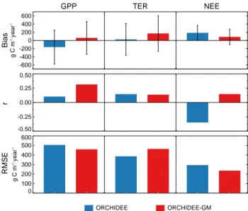
For annual CO2 fluxes, when pooling all the site-years,
ORCHIDEE-GM performs better (lower bias, higher r and lower RMSE) than ORCHIDEE for GPP and NEE (Fig. 8). For example, the NEE bias and RMSE in ORCHIDEE-GM is reduced by 53 % and 20 % respectively, compared to ORCHIDEE. Yet, the simulation of TER is not improved in ORCHIDEE-GM and its bias is even larger than OR-CHIDEE, which could be attributable to two “anomalous” sites (ES-VDA and HU-Bug).
4.3.3 Estimation of C export and NBP
ORCHIDEE-GM has the ability to simulate C exports (Ta-ble 4), e.g., forage production (yield), CH4 emissions and
animal products (i.e., milk) that can be evaluated against independent data. At cut sites, ORCHIDEE-GM gener-ates 718, 336 and 330 g DM m−2yr−1 for DE-Gri, IT-MBo
and PT-Mi2, respectively, which is within a range of 0.88 and 2.26 factor of the observed values (317, 265 and 374 g DM m−2yr−1). For annual animal intake, inter-site dif-ferences are large because of site-dependent grazing inten-sity. For example, the low intake values at both IT-Amp and PT-Mi2 sites are mainly attributable to extensive grazing dur-ing the winter. In addition, both animal respiration and en-teric CH4emissions produced by ORCHIDEE-GM generally
show the same pattern as animal intake (Table 4), which are as a function of animal intake and the time period the animals stay in the field.
After accounting for C export (input) from (to) the site, ORCHIDEE-GM estimates a positive NBP of 37 ± 30 gC m−2yr−1 (P < 0.01) over the 11 sites, which is
comparable to the previous estimate (57 ± 34 gC m−2yr−1)
by Schulze et al. (2009) and lower than that (104 ± 34 gC m−2yr−1) from the GREENGRASS network (Sous-sana et al., 2007). At both intensive and extensive grazed sites, a positive NBP indicative of a net annual carbon sink (18–95 gC m−2yr−1) is found in ORCHIDEE-GM. How-ever, at sites dominated by cutting (including mixed site IT-Amp and PT-Mi2), NBP is modeled to be less than grazed sites or even close zero.
5 Discussion
5.1 Model performance for biometric variables
The addition of an age-dependency of SLA allows intra-annual SLA variation to be modeled in ORCHIDEE-GM, contrary to ORCHIDEE. A rapid increase in SLA during the growing season (Fig. 3) stems from the sprouting of
0 1 2 3 g C m -2 day -1 0 1 2 3 g C m -2 day -1 0 1 2 3 g C m -2 day -1
CH-Oe1 DE-Gri IT-MBo ES-VDA FR-Lq1 FR-Lq2 HU-Bug IE-Dri UK-EBu IT-Amp PT-Mi2
0 1 2 3 g C m -2 day -1 0 1 2 3 g C m -2 day -1 0 1 2 3 g C m -2 day -1
CH-Oe1 DE-Gri IT-MBo ES-VDA FR-Lq1 FR-Lq2 HU-Bug IE-Dri UK-EBu IT-Amp PT-Mi2
Inter-monthly Variability (bin C) Seasonal-Annual Variability (bin B)
RMSE GPP TER NEE GPP TER NEE
CUT GRAZED MIX TOT
ORCHIDEE ORCHIDEE-GM
1035
Fig. 7. Barplot of the root mean squared error (RMSE)
be-tween modeled and observed CO2 fluxes (GPP, TER and NEE)
on seasonal–annual variability and intermonthly variability. Three management types (cut, grazed and mix-managed) are distin-guished. TOT: the mean RMSE and its standard deviation based on all the sites.
new leaves (age class 1 with higher SLA) after cut or dur-ing the grazdur-ing, which helps the plants to capture photosyn-thetic sources and increase the LAI with a relatively small amount of biomass. ORCHIDEE-GM can better reproduce intra-annual variation in biometric variables (LAI and AGB) than ORCHIDEE. This improvement is more noticeable at cut sites than at grazed sites. It could be related to the diffi-culty for ORCHIDEE-GM in accounting for continuous dis-turbance and its induced complex animal–vegetation interac-tions (Vuichard et al., 2007a).
5.2 Model performance for CO2fluxes
ORCHIDEE-GM reproduces intra-annual fluctuations of CO2fluxes significantly affected by grassland management,
either cut (Fig. 4) or grazed (Fig. 5). A better model
GPP -600 -400 -200 0 200 400 600 g C m -2 year -1 TER NEE -0.50 -0.25 0.00 0.25 0.50 0 100 200 300 400 500 600 g C m -2 year -1 Bias r RMSE ORCHIDEE ORCHIDEE-GM 1037 Figure 8 1038
Fig. 8. Statistical performance of models on an interannual scale
for CO2 fluxes (GPP, TER and NEE). Bias: mean model bias
(modeled–observed, gC m−2yr−1) over all site-years, error bar presents the standard deviation of biases; r: correlation between observed and modeled interannual variability; RMSE: root mean squared error for interannual variability in annual totals of CO2
fluxes.
performance in ORCHIDEE-GM compared to ORCHIDEE on intermonthly and seasonal–annual scales is found for NEE and GPP. This further justifies the necessity to incorporate management processes in order to calculate the CO2
ex-change on European grasslands, e.g., for being used as a bet-ter prior of atmospheric CO2 inversions. In addition, an
in-crease in the ability to reproduce NEE at timescales of weeks to year can be attributed to a better simulation of GPP rather than TER that improves marginally. This might be due to the modeling issue of soil organic matter initial disequilib-rium (Carvailhais et al., 2008). Improved GPP simulation by ORCHIDEE-GM comes from more accurate prediction of plant growth under management. However, the main com-ponent of TER is soil respiration. It is highly sensitive to soil organic matter amount, which is initialized by the same soil C module in ORCHIDEE rather than by field observations in this study.
Although ORCHIDEE-GM performs better on both timescales, systematically better at cut sites than at grazed sites, the improvement at grazed sites are more noticeable on the seasonal–annual than on the intermonthly timescales. This illustrates the fact that cut and grazing practices have different influences in the temporal variation of NEE, and that grazing has more impact on seasonal–annual than on in-termonthly timescales. The large amplitude on inin-termonthly timescale (Fig. 6) indicates that the intense sporadic distur-bance, e.g., cut, could also significantly influence CO2fluxes.
5.3 Sources of model–data discrepancies
5.3.1 Initial soil organic matter
All simulations in this study start from modeled steady state, then an arbitrate management history (e.g., 40 yr), rather than based on real soil C conditions, since the latter would require more detailed data on initial C pools of different turnover rates or on site history for the model to simulate the initial value of each carbon pool, compared to what is available. This initialization procedure may cause certain model–data discrepancies.
At CH-Oe1, for example, lower TER is simulated in ORCHIDEE-GM than the observations, which probably re-sults from the simulated low soil organic C and low litter input. Before the year 2002, this site was exposed to a ley– arable rotation management with a nitrogen fertilization of 110 kgN ha−1yr−1. ORCHIDEE-GM simulates a lower soil organic C (12.3 kgC m−2 after 40 yr of spin-up 2) than ob-served (18.3 kgC m−2in 2004, Ammann et al., 2009). More-over, a larger C export (426 gC m−2yr−1)than the observa-tion (∼ 350 gC m−2yr−1)is also found in ORCHIDEE-GM, and then less biomass has thus been left as the litter input.
5.3.2 Site specific parameters
As in other DGVMs, ORCHIDEE simulates an average plant and consequently it only defines average plant functional traits for each PFT, such as mean SLA, the maximal rate of carboxylation (Vcmax)and the light saturate rate of
elec-tron transport (Jmax). However, these traits are highly
site-specific. Plants allocate N to maintain a balance between Vcmaxand Jmax(usually with a close correlation of Jmax≈
2 × Vcmax, Wullschleger, 1993), which are both dependent
on leaf N concentrations and potentially limit photosynthe-sis (Chen et al., 1993). Nutrient (most notably N) limitation also strongly impacts the whole-plant leaf area (Poorter et al., 2009). Then, the soil N availability could be a strong lim-itation of plant growth. ORCHIDEE cannot fully consider the coordination of leaf nitrogen distribution due to the lack of nitrogen cycle, thus preventing simulations of these site-specific parameters.
This model deficiency in capturing site-specific param-eters might introduce the errors in carbon simulations. It can be exemplified by calibrating SLAmax and Vcmax of
ORCHIDEE-GM based on in situ measurements (mean SLA and Vcmax)available at two sites: (i) the intensively grazed
and highly fertilized grassland FR-Lq1, and (ii) the exten-sively grazed grassland FR-Lq2. Our analysis shows that the model errors in GPP, as well as in TER and NEE, are re-duced when site-specific parameter values are used. At FR-Lq1, the RMSE reductions are 8.5 %, 8.9 % and 2.5 % for GPP, TER and NEE, respectively. At FR-Lq2, optimized pa-rameters improve model performance on GPP, TER and NEE (with RMSE reducing 6.0 %, 3.4 % and 3.5 %, respectively).
Our results indicate that wrong-setting values of site-specific parameters (e.g., SLAmaxand Vcmax)could be one of sources
for model–data disagreement. Interestingly to note is that these two parameters are tightly correlated with leaf N con-centrations that are linked to N fertilizer inputs on the fields (Ordoñez et al., 2009).This implies that SLAmaxand Vcmax
could be potentially prescribed to vary spatially as a func-tion of easily available N fertilizer statistical data in future regional simulations.
5.3.3 Observation uncertainties
For CO2 fluxes, NEE is directly measured by
eddy-covariance technique, but with certain site-dependent ran-dom errors from the measurements instruments, the stochas-tic nature of turbulence and varying footprint (area that influences the measurement) (e.g., Hollinger et al., 2004; Richardson and Hollinger, 2005; Richardson et al., 2006; Lasslop et al., 2008). Moreover, the two components GPP and TER are partitioned from NEE by statistical modeling (e.g., Reichstein et al., 2005), which contains certain uncer-tainties (Papale et al., 2006). In addition, certain data gaps due to unfavorable meteorological conditions and system-atic errors in the NEE measurements (e.g., low turbulence occurs in nighttime) can also introduce uncertainties to be
±25 gC m−2yr−1(Moffat et al., 2007). All of these can con-tribute to the observed model–data discrepancies.
5.4 A complete view of NBP
In managed grasslands, the assimilated C by photosynthesis is not only used for ecosystem metabolism but exported by harvest, animal respiration and animal products. After the in-troduction of management, ORCHIDEE-GM is able to sim-ulate forage yield, herbage consumption, animal products (e.g., milk), animal respiration and animal CH4 emissions.
These new variables combined with organic C fertilizer ap-plied on the field could provide a more complete view of grasslands C fluxes for applications of the model on a grid. The added organic fertilizer is also considered given the fact that it could play an important role in some intensively man-aged sites on sustaining soil fertility (e.g., CH-Oe1, IE-Dri, and UK-EBu). The 11 site simulations of this study show that European grasslands generally are C sink (positive NBP). At grazed grasslands, both C export in the form of milk produc-tion and CH4emissions by animals constitute only a minor
part of net primary production (NPP), and this means that NBP mainly depends on NPP. On the contrary, the cut sites accumulate less C in soils because a large part of NPP has been exported as forage production. Given a lower C usage at grazed grasslands than that at cut grasslands, the NBP differ-ence between them indicates a possible relationship between the C usage and NBP found by Soussana et al. (2007). This same relationship is also found within cut grasslands and grasslands having both grazing and cutting (Table 4). The
Table 4. Model output related to management from ORCHIDEE-GM. Yield, mean annual forage production (dry matter, g m−2yr−1); intake, mean annual grass mass digested by animals (dry matter, g m−2yr−1); respiration, mean annual animal respiration (C, g m−2yr−1); MilkC, mean annual C export in milk production (C, g m−2yr−1); CH4, mean annual enteric CH4emission (C-CH4, g m−2yr−1); NBP,
net biome production (C, g m−2yr−1).
Management Site Yield Intake Respiration MilkC CH4 NBP
Cutting CH-Oe1 975 – – – – 3 DE-Gri 760 – – – – 10.0 IT-MBo 288 – – – – 21.0 Grazing ES-VDA – 58 11.0 4.0 0.8 60.1 FR-Lq1 – 374 71.3 – 3.9 41.6 FR-Lq2 – 250 47.6 – 0.7 57.7 HU-Bug – 176 33.5 15.0 2.3 37.9 IE-Dri – 272 51.8 20.7 3.5 68.1 UK-EBu – 231 44.1 14.3 3.9 94.5 Cutting/grazing IT-Amp 301 65 12.5 3.4 1.8 3.5 PT-Mi2 110 43 8.2 2.6 0.8 11
results from paired sites (FR-Lq1 and FR-Lq2, see Table 4) further confirm that increased C usage (higher herbage in-take at extensively grazed grassland, FR-Lq1) may diminish C sequestration (lower NBP) in managed grasslands, given the fact that intensive grazing reduces LAI and further de-cline NPP (Parsons et al., 1983).
Fully accounting for NBP still takes into account dissolved organic/inorganic (DOC/DIC) C losses to water, which, how-ever, is not implemented in ORCHIDEE-GM. If the av-erage DOC/DIC loss estimated at European scale (11 ± 8 gC m−2yr−1; Siemens, 2003) reduced the NBP by 30 %,
the residual NBP (positive, P < 0.05) still indicates a C se-questration in European managed grasslands.
However, it should be noted that our estimation of NBP is biased by the fact that the model initialization of soil C pools is not realistic. Only long-term simulation with pre-cise management history or initialization based on prepre-cise soil organic C (e.g., the European Soil Database; Panagos et al., 2012) can avoid this uncertainty when running the model on a grid for future applications. Nevertheless, a more com-plete picture of NBP provided by ORCHIDEE-GM enables us to separate the role of grassland management from those of other factors (e.g., CO2, climate and land use) in the
at-tribution of the grassland C sequestration (Soussana et al., 2010).
6 Conclusions
This paper is an attempt to realistically represent the impact of management on the C fluxes of European grasslands in a DGVM. We developed a new model, ORCHIDEE-GM, in-tegrating a management module from a grassland specific model (PaSim) and evaluated its results at 11 European sites. Generally, ORCHIDEE-GM is better able to reproduce intra-annual variation of LAI, AGB, and CO2fluxes (GPP, TER,
and NEE) induced by cut or grazing practices. Model–data discrepancies can be attributed to lack of data to initialize soil C pools, to CO2fluxes observation uncertainties and to
some site-specific parameter values. The optimization of N related parameters (SLA, Vcmax, and Jmax)in
ORCHIDEE-GM reduces the model–data misfit at sites where it was per-formed. However, we should state that this study is not de-signed for fully bridging the gap in C fluxes simulations but more for understanding the contributing effect of improved management practices to C fluxes simulations in temperate grassland.
The simulated C fluxes of forage yield, herbage consump-tion, animal products (milk), animal respiration and methane emissions by ORCHIDEE-GM give a more complete pic-ture of NBP in managed temperate grasslands. This model with its realistic management process could enable us to re-examine the C balance in the regions, such as Europe and China, which distribute a large area of managed temperate grasslands. Furthermore, it could also be adopted to under-stand the responses of forage yield or other GHGs to the on-going climate change and investigate the feedback between surface albedo and air temperature induced by management practices (cut and grazing).
Acknowledgements. This work was made possible through the
support of the CARBOEUROPE-IP and Nitroeurope project to eddy-covariance flux sites. Special thanks go to PIs for giving us access to their ancillary and flux data. We would like to thank Ship-ing Chen, who provided ancillary information for sites in China (CN-Du2, CN-Dwu, CN-Xi1 and CN-Xi2). We also acknowledge the PhD funding by Commissariat à l’énergie atomique (CEA) in France. Finally, we greatly thank Ray Anderson and the anonymous reviewers for their constructive comments on the manuscript. Edited by: M.-H. Lo
The publication of this article is financed by CNRS-INSU.
References
Abril, A. and Bucher, E. H.: The effects of overgrazing on soil mi-crobial community and fertility in the chaco dry savannas of Ar-gentina, Appl. Soil Ecol., 12, 159–167, 1999.
Ammann, C., Spirig, C., Leifeld, J., and Neftel, A.: Assessment of the nitrogen and carbon budget of two managed temperate grass-land fields, Agr. Ecosyst. Environ., 133, 150–162, 2009. Baldocchi, D., Falge, E., Gu, L., Olson, R., Hollinger, D., Running,
S., Anthoni, P., Bernhofer, C., Davis, K., Evans, R., and Fuentes, J.: FLUXNET: A New Tool to Study the Temporal and Spatial Variability of Ecosystem-Scale Carbon Dioxide, Water Vapor, and Energy Flux Densities, B. Am. Meteorol. Soc., 82, 2415– 2434, 2001.
Berg, B. and Matzner, E.: Effect of N deposition on decomposition of plant litter and soil organic matter in forest systems, Environ. Rev. 5, 1–25, 1997.
Béziat, P., Ceschia, E., and Dedieu, G.: Carbon balance of a three crop succession over two cropland sites in south west france, Agr. Forest. Meteorol., 149, 1628–1645, 2009.
Bondeau, A., Smith, P. C., Zaehle, S., Schaphoff, S., Lucht, W., Cramer, W., Gerten, D., Lotze-Campen, H., Mueller, C., Reich-stein, M., and Smith, B.: Modelling the role of agriculture for the 20th century global terrestrial carbon balance, Global. Change. Biol., 13, 679–706, 2007.
Broomhead, D. S. and King, G. P.: Extracting qualitative dynamics from experimental-data, Physica D, 20, 217–236, 1986. Byrne, K. A., Kiely, G., and Leahy, P.: Carbon sequestration
de-termined using farm scale carbon balance and eddy covariance, Agr. Ecosyst. Environ., 121, 357–364, 2007.
Carvalhais, N., Reichstein, M., Seixas, J., Collatz, G. J., Pereira, J. S., Berbigier, P., Carrara, A., Granier, A., Montagnani, L., Papale, D., Rambal, S., Sanz, M. J., and Valentini, R.: Implications of the carbon cycle steady state assumption for biogeochemical mod-eling performance and inverse parameter retrieval, Global Bio-geochem. Cy. 22, GB2007, doi:10.1029/2007GB003033, 2008. Chen, D. X., Hunt, H. W., and Morgan, J. A.: Responses of a C3
and C4 perennial grass to CO2enrichment and climate change:
Comparison between model predictions and experimental data, Ecol. Model., 87, 11–27, 1996.
Chen, J. L., Reynolds, J. F., Harley, P. C., and Tenhunen, J. D.: Co-ordination theory of leaf nitrogen distribution in a canopy, Oe-cologia, 93, 63–69, 1993.
Ciais, P., Reichstein, M., Viovy, N., Granier, A., Ogee, J., Allard, V., Aubinet, M., Buchmann, N., Bernhofer, C., Carrara, A., Cheval-lier, F., De Noblet, N., Friend, A. D., Friedlingstein, P., Grun-wald, T., Heinesch, B., Keronen, P., Knohl, A., Krinner, G., Lous-tau, D., Manca, G., Matteucci, G., Miglietta, F., Ourcival, J. M., Papale, D., Pilegaard, K., Rambal, S., Seufert, G., Soussana, J. F., Sanz, M. J., Schulze, E. D., Vesala, T., and Valentini, R.: Europe-wide reduction in primary productivity caused by the heat and drought in 2003, Nature 437, 529–533, 2005.
Conant, R. T., Paustian, K., and Elliott, E. T.: Grassland manage-ment and conversion into grassland: Effects on soil carbon, Ecol. Appl., 11, 343–355, 2001.
Dolman, A. J., Noilhan, J., Durand, P., Sarrat, C., Brut, A., Piguet, B., Butet, A., Jarosz, N., Brunet, Y., Loustau, D., Lamaud, E., Tolk, L., Ronda, R., Miglietta, F., Gioli, B., Magliulo, V., Es-posito, M., Gerbig, C., Korner, S., Glademard, R., Ramonet, M., Ciais, P., Neininger, B., Hutjes, R. W. A., Elbers, J. A., Macatan-gay, R., Schrems, O., Perez-Landa, G., Sanz, M. J., Scholz, Y., Facon, G., Ceschia, E., and Beziat, P.: The CARBOEURPOE re-gional experiment strategy, B. Am. Meteorol. Soc., 87, 1367– 1379, 2006.
Ducoudre, N. I., Laval, K., and Perrier, A.: Sechiba, a new set of parameterizations of the hydrologic exchanges at the land atmo-sphere interface within the lmd atmospheric general-circulation model, J. Climate, 6, 248–273, 1993.
Elsner, J. B. and Tsonis, A. A.: Singular Spectrum Analysis: A New Tool in Time Series Analysis, 164 pp., Plenum, New York, 1996. Falge, E., Baldocchi, D., Olson, R. J., Anthoni, P., Aubinet, M., Bernhofer, C., Burba, G., Ceulemans, R., Clement, R., Dolman, H., Granier, A., Gross, P., Grünwald, T., Hollinger, D., Jensen, N.-O., Katul, G., Keronen, P., Kowalski, A., Ta Lai, C., Law, B. E., Meyers, T., Moncrieff, J., Moors, E., Munger, J. W., Pile-gaard, K., Rannik, Ü., Rebmann, C., Suyker, A., Tenhunen, J., Tu, K., Verma, S., Vesala, T., Wilson, K., and Wofsy, S.: Gap filling strategies for defensible annual sums of net ecosystem ex-change, Agr. Meteorol., 107, 43–69, 2001.
Fearnside, P. M. and Barbosa, R. I.: Soil carbon changes from con-version of forest to pasture in brazilian amazonia, Forest. Ecol. Manage., 108, 147–166, 1998.
Feddema, J., Oleson, K., Bonan, G., Mearns, L., Washington, W., Meehl, G., and Nychka, D.: A comparison of a GCM response to historical anthropogenic land cover change and model sensitivity to uncertainty in present-day land cover representations, Clim. Dynam., 25, 581–609, 2005.
Foley, J. A., DeFries, R., Asner, G. P., Barford, C., Bonan, G., Car-penter, S. R., Chapin, F. S., Coe, M. T., Daily, G. C., Gibbs, H. K., Helkowski, J. H., Holloway, T., Howard, E. A., Kucharik, C. J., Monfreda, C., Patz, J. A., Prentice, I. C., Ramankutty, N., and Snyder, P. K.: Global consequences of land use, Science, 309, 570–574, 2005.
Foy, J. K., Teague, W. R., and Hanson, J. D.: Evaluation of the up-graded SPUR model (SPUR2.4), Ecol. Model., 118, 149–165, 1999.
Ghil, M., Allen, M. R., Dettinger, M. D., Ide, K., Kondrashov, D., Mann, M. E., Robertson, A. W., Saunders, A., Tian, Y., Varadi, F., and Yiou, P.: Advanced spectral methods for climatic time series, Rev. Geophys., 40, 1003, doi:10.1029/2000RG000092, 2002. Gilmanov, T. G., Soussana, J. E., Aires, L., Allard, V., Ammann,
C., Balzarolo, M., Barcza, Z., Bernhofer, C., Campbell, C. L., Cernusca, A., Cescatti, A., Clifton-Brown, J., Dirks, B. O. M., Dore, S., Eugster, W., Fuhrer, J., Gimeno, C., Gruenwald, T., Haszpra, L., Hensen, A., Ibrom, A., Jacobs, A. F. G., Jones, M. B., Lanigan, G., Laurila, T., Lohila, A., Manca, G., Marcolla, B., Nagy, Z., Pilegaard, K., Pinter, K., Pio, C., Raschi, A., Ro-giers, N., Sanz, M. J., Stefani, P., Sutton, M., Tuba, Z., Valentini, R., Williams, M. L., and Wohlfahrt, G.: Partitioning European grassland net ecosystem CO2exchange into gross primary