HAL Id: hal-01678430
https://hal.archives-ouvertes.fr/hal-01678430
Submitted on 10 May 2018
HAL is a multi-disciplinary open access
archive for the deposit and dissemination of
sci-entific research documents, whether they are
pub-lished or not. The documents may come from
teaching and research institutions in France or
abroad, or from public or private research centers.
L’archive ouverte pluridisciplinaire HAL, est
destinée au dépôt et à la diffusion de documents
scientifiques de niveau recherche, publiés ou non,
émanant des établissements d’enseignement et de
recherche français ou étrangers, des laboratoires
publics ou privés.
Optics in Tandem with HST on a Faint Halo Object
T. K. Fritz, S. T. Linden, P. Zivick, N. Kallivayalil, R. L. Beaton, J. Bovy, L.
V. Sales, T. Sohn, D. Angell, M. Boylan-kolchin, et al.
To cite this version:
T. K. Fritz, S. T. Linden, P. Zivick, N. Kallivayalil, R. L. Beaton, et al.. The Proper Motion of Pyxis:
The First Use of Adaptive Optics in Tandem with HST on a Faint Halo Object. The Astrophysical
Journal, American Astronomical Society, 2017, 840 (1), �10.3847/1538-4357/aa6b5a�. �hal-01678430�
arXiv:1611.08598v3 [astro-ph.GA] 1 Apr 2017
THE PROPER MOTION OF PYXIS: THE FIRST USE OF ADAPTIVE OPTICS IN TANDEM WITH HST ON A FAINT HALO OBJECT
T. K. Fritz,1 S. T. Linden,1P. Zivick,1 N. Kallivayalil,1R. L. Beaton,2 J. Bovy,3, 4, 5L. V. Sales,6 S. T. Sohn,7 D. Angell,1M. Boylan-Kolchin,8E. R. Carrasco,9 G. J. Damke,1 R. I. Davies,10 S. R. Majewski,1B. Neichel,11
and R. P. van der Marel7
1Department of Astronomy, University of Virginia, Charlottesville, 530 McCormick Road, VA 22904-4325, USA 2The Observatories of the Carnegie Institution for Science, 813 Santa Barbara St., Pasadena, CA 91101, USA
3Department of Astronomy & Astrophysics at University of Toronto, 50 St. George Street M5S 3H4 Toronto, Ontario, Canada 4
Center for Computational Astrophysics, 162 5th Ave, New York, New York 10010, USA 5Alfred P. Sloan Fellow
6Department of Physics and Astronomy, University of California Riverside, 900 University Avenue, CA 92507, USA 7Space Telescope Science Institute, 3700 San Martin Drive, Baltimore, MD 21218, USA
8The University of Texas at Austin, Department of Astronomy, 2515 Speedway, Stop C1400,Austin, Texas 78712, USA 9Gemini Observatory, Southern Operations Center, AURA, Casilla 603, La Serena, Chile
10Max Planck Institut f¨ur Extraterrestrische Physik, Postfach 1312, D-85741, Garching, Germany 11LAM - Laboratoire dAstrophysique de Marseille, 38, rue Frederic Joliot-Curie, 13388 Marseille, France
ABSTRACT
We present a proper motion measurement for the halo globular cluster Pyxis, using HST/ACS data as the first epoch, and GeMS/GSAOI Adaptive Optics data as the second, separated by a baseline of ∼ 5 years. This is both the first measurement of the proper motion of Pyxis and the first calibration and use of Multi-Conjugate Adaptive Optics data to measure an absolute proper motion for a faint, distant halo object. Consequently, we present our analysis of the Adaptive Optics data in detail. We obtain a proper motion of µαcos(δ) =1.09±0.31 mas yr−1 and
µδ =0.68±0.29 mas yr−1. From the proper motion and the line-of-sight velocity we find the orbit of Pyxis is rather
eccentric with its apocenter at more than 100 kpc and its pericenter at about 30 kpc. We also investigate two literature-proposed associations for Pyxis with the recently discovered ATLAS stream and the Magellanic system. Combining our measurements with dynamical modeling and cosmological numerical simulations we find it unlikely Pyxis is associated with either system. We examine other Milky Way satellites for possible association using the orbit, eccentricity, metallicity, and age as constraints and find no likely matches in satellites down to the mass of Leo II. We propose that Pyxis probably originated in an unknown galaxy, which today is fully disrupted. Assuming that Pyxis is bound and not on a first approach, we derive a 68% lower limit on the mass of the Milky Way of 0.95×10¹²M
⊙.
Keywords: proper motions, globular clusters: individual: Pyxis
Corresponding author: T. K. Fritz
1. INTRODUCTION
Of the globular clusters of the Milky Way, Pyxis (Da Costa 1995; Irwin et al. 1995) is one of the most distant (∼ 40 kpc; Sarajedini & Geisler 1996). Even though the relatively high line-of-sight extinction of E(B-V)≈ 0.25 (Dotter et al. 2011) adds a large uncer-tainty on this measurement, Pyxis clearly resides in the halo. Pyxis has a metallicity of [Fe/H]= −1.45 ± 0.1; (Palma et al. 2000; Dotter et al. 2011; Saviane et al. 2012) and, from comparison to theoretical isochrones, is 11.5±1 Gyr old, roughly 2 Gyr younger than in-ner Milky Way globular clusters of the same metallic-ity (Dotter et al. 2011; Saviane et al. 2012). Together, these measurements suggest that Pyxis belongs to the somewhat younger population of halo globular clusters that have likely been accreted by the Milky Way (Zinn 1993).
Indeed, the three-dimensional location of Pyxis is quite suggestive of a complicated origin. Irwin et al. (1995) speculate that Pyxis originates from the Large Magellanic Cloud (LMC), based on the proximity of Pyxis to its orbital plane. More recently,Koposov et al. (2014) discovered the ATLAS stellar stream and three globular clusters, including Pyxis, were considered po-tential progenitors of the stream. The proper motions of both NGC 7006 and M 15 were inconsistent with the implied orbit of the stream, and Pyxis, with no proper motion measurement, became the most likely candidate. Both scenarios, an LMC origin and that Pyxis is being tidally stripped, can be tested with a proper motion measurement.
Validation of these scenarios has larger implications than just the origin of Pyxis. Detailed observations of stellar streams coupled with numerical simulations can be used to constrain the potential of the Milky Way halo (Koposov et al. 2010; K¨upper et al. 2015; Bovy et al. 2016a) as well as the mass function of subhalos within it (Yoon et al. 2011;Erkal et al. 2016;Bovy et al. 2016b). Longer streams improve such constraints: currently, the ATLAS stream is rather short (12◦ Koposov et al.
(2010)), but if Pyxis is its progenitor system, then it would be one of the longest streams currently traced within the Milky Way halo. Three-dimensional motions for halo objects, like Pyxis, can also be used to constrain the rotation curve at relatively large distances and thus the mass of the Milky Way.
Absolute proper motions for halo objects have been obtained with ground-based seeing-limited observations with long time baselines (≥ 15 years; e.g.,Dinescu et al. 1999; Fritz & Kallivayalil 2015), or with the Hub-ble Space Telescope (HST) (e.g., Piatek et al. 2007; Kallivayalil et al. 2013), which permits measurements
over shorter time scales due to its better spatial res-olution (∼3-5 years). Ground-based adaptive optics have the potential to provide the HST-quality spa-tial resolution to enable shorter baseline proper mo-tion measurements from the ground. Indeed, adap-tive optics techniques have been well-established for proper motions (e.g., Gillessen et al. 2009) using sin-gle conjugated adaptive optics systems. Now, multi-conjugated adaptive optics (MCAO) systems provide a larger field of view and have already been used for rela-tive proper motions (Ortolani et al. 2011;Massari et al. 2016a), in which the motion of a source is measured relative to another object in the Milky Way halo. The larger field-of-view of MCAO makes it possible to now also find faint background galaxies in the same im-ages which can be used to get absolute motions, like what has been done already with seeing-limited im-ages (e.g., Dinescu et al. 1997) and with HST (e.g., Kalirai et al. 2007;Sohn et al. 2013;Pryor et al. 2015). The GeMS/GSAOI system in operation at Gemini South (Rigaut et al. 2014; Carrasco et al. 2012) is the first AO system that combines the large sky-coverage of laser guide-stars with the wide diffraction-limited field-of-view of MCAO (Davies & Kasper 2012) enabling ob-servations of targets without bright stars which are necessary for a system without lasers.
In an on-going multi-year Gemini Large Program (LP-GS-2014B-2; PI: Fritz1), we are using the GeMS/GSAOI
system to measure absolute proper motions for a set of Milky Way halo tracers, including Pyxis. While sys-tems like GeMS/GSAOI are currently rare, planned in-strumentation for 30-meter class facilities include wide-field AO imaging (one example being MICADO, see Davies et al. 2016, for details) and AO-based proper mo-tions from the ground will become more fruitful. The development of proper motion analysis techniques that use such instrumentation, thus, are valuable for future efforts.
The Gemini Large program is still ongoing (we require 3 year baselines) and the second epoch of AO imaging for Pyxis has not yet been obtained. We can, however, utilize archival optical HST imaging, taken in 2009, as our first epoch. This sets a five year baseline between the first optical observations and our second near-infrared AO imaging.
The paper is organized as follow: In Section 2 we present the data used in this study and in Section3 we discuss our techniques to measure photometry and po-sitions in our datasets. We describe the methods used
1 A program summary is available at the following URL
in the measurement of the proper motion of Pyxis in Section 4. In Section 5 we use the proper motion to constrain its orbit and to explore the possible origin of Pyxis. We conclude in Section6.
2. IMAGING DATA SET
In this section, we describe the imaging used to mea-sure the proper motion of Pyxis. Technical details for our imaging datasets are summarized in Table1.
2.1. HST Imaging
The first epoch consists of archival HST ACS/WFC F 606W and F 814W data2. These images were obtained
in 2009 (MJD = 55115.7) and provide a sufficient base-line in combination with our AO imaging. In each band, there are 4 ‘long’ images of about 540 seconds exposure time, which we use for the main astrometry. To recover photometry for bright stars that were saturated in the long exposure images, we use single short exposure (≈53 s) images obtained in both filters. The individual frames are dithered by up to 17′′, such that not all sources are
contained in each individual exposure.
For astrometry and photometry, we use the flc data products produced by the MAST pipeline. The flc data products are bias-subtracted, dark-subtracted, flat-fielded flt images with the pixel-based charge transfer efficiency (CTE) correction applied (Avila et al. 2016). The flc images have a pixel scale of 0.05′′pixel−1. The
pipeline produced drz images for each filter are also used for visual inspection. For some purposes, we create our own chip-merged frames using a chip-separation of 50 pixels between the two ACS chips.
Generally, cosmic rays are flagged by the CALACS pipeline in individual flt/flc exposures in a given filter by comparison against other images of the same filter. The dithering between these exposures, however, leaves some area of the chip without a CR comparison image. In these cases, we flag cosmic rays manually by compar-ing this area to its counterpart in the other filter. The weight of pixels affected by cosmic rays is set to zero so that they do not affect our analysis.
2.2. Gemini Imaging
For the second epoch, we use the wide field AO system GeMS/GSAOI at Gemini South (Rigaut et al. 2014; Carrasco et al. 2012). The Gemini Multi-Conjugate Adaptive Optics System (GeMS) is a multi-conjugate adaptive optics system (MCAO) designed for the Gemini-S telescope. For technical details on the AO sys-tem, we refer the reader toRigaut et al. (2014) and for
2Proposal ID GO11586 PI-Aaron Dotter.
on-sky performance toNeichel et al.(2014). The Gem-ini South Adaptive Optics Imager (GSAOI) instrument is designed to work with GeMS and provides diffraction limited images over the 0.9 to 2.5 µm wavelength range. The image plane is filled with a 2× 2 mosaic of Rock-well HAWAII-2RG 2048×2048 pixel arrays producing a 85′′
× 85′′ field-of-view at 0.02′′ pixel−1 resolution.
For additional technical details on GSAOI, we refer the reader toMcGregor et al.(2004) for instrument design and toCarrasco et al.(2012) for commissioning perfor-mance.
The Pyxis field was chosen to both meet the techni-cal requirements of the AO system (three nearby bright, R< 15.5 mag, stars for tip-tilt and plate-scale mode vari-ations) and to provide maximal overlap with the HST frame for data validation and comparison purposes. We avoided the central part of the cluster where the density is high and background galaxies are more difficult to identify and fully characterize. The science data were obtained on 2015 January 7 (MJD = 57030.3) under good conditions, giving a 5-year baseline between the first (HST) and second (AO) epoch of imaging. The data set consists of 30 science K′-band images of 120
sec-onds each. In addition, off-field images were observed for sky subtraction. The observations of the science frames were divided in five groups of six images each. Within each group, the science images were observed using a small dither-steps (< 1′′) with the tip-anisoplanatic loop
closed (accurate astrometry of the NGS probes in Cano-pus is derived before the loop is closed). Larger dithers of 5′′ were used between each group to cover the gap
regions between detectors and to improve the derived distortion solution for the GeMS/GSAOI data. Offsets above 1′′ requires to open tip- anisoplanatic loop, apply
the large offset and re-do the astrometry of the NGS Canopus probes, before the observations can be contin-ued. The sky images were obtained between the groups. We reduce the individual GSAOI frames in the stan-dard way using domeflats, dead pixel masks, and sky images. The sky is constructed from off-Pyxis images because the source density for on-Pyxis images is too high. The data is also corrected for non-linearity and craters caused by bright stars by setting the affected pixels to values above the saturation limits. We con-struct noise maps from the data and find these to be dominated by sky noise.
The four chips of the GSAOI images are arranged in a 2×2 grid with average separations of 120 pixels in both the x- and y- image dimensions. For the derivation of the distortion corrections, we treat the four chips mostly independently, see Section 4.2. For photometry and pixel positions, however, there are insufficient stars in
Table 1. Summary of Imaging Data
Telescope+Camera Filter MJD ExpTime [s] Nobs Resolution Notes
days [s] ′′pixel−1
HST+ACS/WFC F606W 55115.7 517 4 0.05
55115.7 50 1 0.05 Used to recover saturated stars
F814W 55115.7 557 4 0.05
55115.7 55 1 0.05 Used to recover saturated stars
Gemini-S + GeMS/GSAOI K′ 57030.3 120 30 0.02 Obtained in 5 6-image sets.
Figure 1. Pyxis images: (left) 3-color image of the three high-resolution images used in this study (blue F 606W , green F814W , red K′); (right) GMOS-S i-band image, the GSAOI field is indicated in red and the HST field in blue. The GMOS-S image was also obtained as part of our Long Term Gemini program, but is not used for science in this paper.
any individual chip for the derivation of a point-spread-function (PSF). Thus, we must combine the four chips into a single frame for each exposure using the average chip separation. Our procedure assumes that the chips are perfectly aligned, which is not exactly true, and we will evaluate the impact of this misalignment in our PSF modeling (Section 3.2.2).
Most of our analysis is performed on the individual frames, but for some purposes, like source identification, we use the higher signal-to-noise combined mosaic image of the 30 individual science frames. The mosaic-ed com-bined image is constructed using the package THELI3.
Astrometry and distortion correction are done using the program ”SCAMP” (Bertin 2006) called from THELI.
3
Available: https://www.astro.uni-bonn.de/theli/ (Erben et al. 2005;Schirmer 2013)
The reference catalog is constructed from an archival image obtained in J-band with the Visible and In-frared Survey Telescope for Astronomy (VISTA) and the VISTA InfraRed Camera (VIRCAM) located at Paranal Observatory. After the astrometry and distortion cor-rection are derived, the sky background subtraction is performed on individual images in order to achieve a ho-mogeneous zero background level across the multi-array GSAOI frames. Finally the images are resampled to a common position, mosaic-ed and then combined us-ing the software Swarp (Bertin 2010) called from in-side THELI. The internal astrometric errors in the final co-added mosaic-ed image are less than 10 mas. We did evaluate the use of this higher signal-to-noise im-age for our astrometric analysis, but found the distor-tion correcdistor-tions applied to the individual images before co-addition were not sufficiently precise for our need of
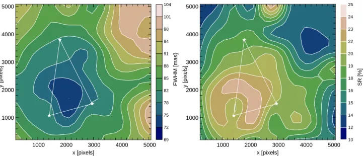
1 mas precision. The individual source shapes, how-ever, were not strongly impacted by the residual distor-tion in the co-added image, and thus the image provides higher S/N for morphology assessment than the individ-ual frames. In Figure2, we demonstrate the quality of our mosaic with the FWHM and Strehl ratio computed across the field of view. As in Neichel et al. (2014) we use Yorick to measure these properties. The correction is relatively good with FWHM< 90 mas SR> 15% over most of the field.
2.3. Image Overlap
Figure1gives a summary of the imaging used for this project. The left panel of Figure 1 is a color compos-ite image of the overlap between the HST optical and GeMS/GSAOI NIR imaging. Approximately 73% of our GeMS/GSAOI field has HST imaging. The right panel of Figure1 uses a GMOS-S image of Pyxis (located in the center towards the right) showing the locations of the imaging used for this paper. While the HST point-ing is on the center of the Pyxis cluster, our GSAOI field is offset to the North where the stellar density is lower. From visual inspection, the GSAOI images are of overall lower photometric depth than those of HST.
3. PHOTOMETRY AND INITIAL POSITIONS
In this section, we describe the creation of Pyxis astro-metric and photoastro-metric catalogs from the optical HST and near-infrared AO imaging. We sub-divide this pro-cess into the procedures for stellar photometry and those for galaxy photometry. Stellar photometry for HST imaging is described in Section 3.1. For the GSAOI images, we first develop appropriate PSF fitting tech-niques in Section 3.2, which are described in detail in those subsections. Our MCAO PSF is applied to stellar sources in Section 3.3. The estimation of galaxy posi-tions is described in Section 3.4, which is done for HST and AO in concert. We determine corrections to the ini-tial positions using a preliminary distortion correction and evaluate the effect of differential chromatic refrac-tion (DCR) in Secrefrac-tion3.5. This process is summarized in Section3.6.
3.1. Stellar Sources in HST
There exist already well-vetted codes for extracting astrometry and photometry from HST images and we follow those outlined in Anderson & King (2006). For the photometry and astrometry, the flc data products were used instead of the provided drz data products since the latter involve an image resampling that de-grades the astrometry. Starting with the flc images, we perform PSF fitting, utilizing empirical ‘Anderson
Core’ PSFs constructed specifically for the F 606W and F 814W filters byAnderson & King (2006), to create a catalog of pixel positions and photometry of all point sources for all exposures. Both stellar and non-stellar sources are included in this catalog, but the positions for galaxies will be refined by 2-dimensional galaxy fit-ting in Section3.4.
We calibrate the photometry using the STScI pro-vided zero points4of 26.406 and 25.520 mag in F 606W
and F 814W , respectively, and use the 0.5′′ to
infin-ity aperture-correct (0.091 mag in both bands from Sirianni et al.(2005).
3.2. Derivation of AO PSFs Using Stellar Sources In MCAO imaging the PSF varies over the field of view. Thus, the PSF needs to be derived as a func-tion of the coordinate posifunc-tion. Because Starfinder (Diolaiti et al. 2000) derives only 1 PSF per attempt, it is a cumbersome tool to derive the PSF for the full field of view. Further, in our case of a low star den-sity the advantage of Starfinder in the regime of a high star density is not valid. In contrast, the low star den-sity, makes it more difficult to choose a local sample of stars, (as inMeyer et al. 2011;Neichel et al. 2014), with sufficient number and spatial coverage. DAOPHOT (Stetson 1987) was used as an option in other works (Ortolani et al. 2011; Massari et al. 2016a). We here opt to test another option, PSF Extractor (Bertin 2011). First, we have to construct an initial high SNR stellar catalog from which the spatial and time-varying PSF can be derived (Section3.2.1). Second, we use PSF Ex-tractor (PSFeX) to build model PSF grids from which the PSF at any given location can be derived (Section 3.2.2). We evaluate the effectiveness of these models for astrometry in Section 3.2.4. Lastly, we develop model grids on the AO mosaic image for photometry in Section 3.2.5.
3.2.1. Source Classification
Our source list is generated from the THELI-mosaicked GSAOI images as these images set the lim-iting photometric depth of our analysis. For the initial selection of sources, we start with the function find in the dpuser image reduction5, which uses a
globally-derived SNR criterion and FWHM to select stars. After an initial pass, additional SNR criteria based on the local noise around an individual source are applied;
4
They are obtained from http://www.stsci.edu/hst/acs/analysis/ zeropoints/old page/localZeropoints.
5
For more details on dpuser see
1000 2000 3000 4000 5000 1000 2000 3000 4000 5000 69 72 75 78 82 85 88 91 94 98 101 104 FWHM [mas] x [pixels] y [pixels] 1000 2000 3000 4000 5000 1000 2000 3000 4000 5000 10 12 14 15 16 18 19 20 22 23 24 25 SR [%] x [pixels] y [pixels]
Figure 2. Quality characteristics of the Pyxis data: On the left the FWHM is shown as a function of position, the unit is mas; on the right the Strehl Ratio is shown as a function of position, the unit is %. Both are measured on the mosaic image. The white stars of the triangle mark the used tip tilt stars.
this step ensures that most selected stellar sources are real. Lastly, each source is then examined by eye in the images to remove spurious sources, including false detection caused by close saturated stars, image arti-facts, or sky noise, or real sources that are compromised due to any of the previous spurious sources. Thus, our final source list contains visually verified objects that are either stars or galaxies.
Validation and addition of more galaxy candidates continues via a visual inspection of the K′-band
mo-saic. To ease detection of galaxies with lower surface brightness features, we first smooth the K′-band mosaic
with a Gaussian of FWHM= 3 pixels and refine the ini-tial classification of star or galaxy. Galaxy candidates are then fit individually with a two-dimensional Gaus-sian and the fit parameters are compared to those fits of neighboring stars. Only candidates that are clearly different from confirmed stars are considered galaxies in this step. Not all objects are clearly classified with a Gaussian fit and for these borderline cases we also con-sider the fit parameters from the Galfit code (Peng et al. 2002) (more detailed galaxy fitting will be provided in Section 3.4). We compare the χ2 of a PSF fit and a
Sersic fit and the obtained Sersic parameters. We ex-clude sources which are fit better by a Sersic, but for which the Sersic index is large, and the effective radius and the axis ratio are both small. These are unphysical parameters for galaxies and these objects are probably barely-resolved binary stars. Overall, only a few sources are reclassified in the second step. Due to the high spa-tial resolution there remain no borderline cases at the end.
We confirm the classifications with visual inspection of the HST imaging and we exclude a few red galax-ies which are invisible in the HST images. Overall, 52 galaxies are confirmed in the GSAOI footprint. The four saturated stars in the AO imaging are added by hand to our star list. Overall, 450 stars are confirmed in the GSAOI footprint.
We note that both the star and galaxy samples were created conservatively owing to the needs of our anal-ysis for clean samples of stars (for the proper motions) and galaxies (for the astrometric reference frame). The faintest sources (galaxy or stellar) contribute only with a very small weight to the overall analysis and the in-completeness of the sample does not affect our proper motion.
3.2.2. PSF estimation for AO images
We use PSF Extractor (PSFeX;Bertin 2011) to gener-ate PSF models for the GSAOI imaging for use in both astrometry and photometry-based analyses. PSFeX is designed to automatically select point-like sources from SExtractor (Bertin & Arnouts 1996) catalogs and con-struct models of the point spread function (PSF) across an image. PSFeX models PSF variations as a user-defined polynomial function of position in an image. However, PSFex does not work directly on the images themselves. Instead, it operates on SExtractor catalogs that have a small image ‘vignette’ recorded for each de-tection. We will first describe general considerations for using PSFeX before we discuss the detailed generation of our PSF grids for astrometry and photometry.
We start by generating SExtractor catalogs for each of our AO frames. PSFeX automatically pre-selects sources from this SExtractor input catalog that are likely to be stellar based on source characteristics, such as half-light radius and ellipticity, while also rejecting contaminated or saturated objects identified in SExtractor. Each iteration of the PSF modeling consists of computing the PSF, comparing the vignettes to the reconstructed model, and excluding detections that show too much departure between the data and the model. We use a pixel-based Principal Component Analysis to build a χ2-minimized image basis vector to represent the PSF.
PSFeX uses these custom basis vectors to interpolate PSF models at specific locations for an output grid with the same resolution and size as each input GSAOI im-age. Thus, there are two critical inputs for PSFeX: (i) the SExtractor catalog from which sources are selected and (ii) the interpolation scheme used to generate the model output grid.
Our GSAOI images are atypical of the normal PSFeX applications due to a very high degree of PSF variability across the frame and a source density that is overall too low for high-fidelity measurements of that variability. Thus, we bypass the “automatic” selection and used our confirmed stellar sample (Section3.2.1) to optimize the basic PSFeX procedure for our GSAOI data in the fol-lowing ways: (i) we use large image vignettes (VIGNET size and PSF SIZE) of 128x128 pixels, (ii) we require a minimum SNR of 20 in the central pixel, and (iii) we allow for large variations in both the maximum elliptic-ity (0-100%) and FWHM (2.5 - 29.7 pixels) of the model sources. These modifications help to maximize the num-ber of sources PSFeX uses to build the basis vectors and thus improve the accuracy of any higher-order in-terpolation to parts of the image where either the source identification is sparse or the background RMS is larger. The size of the image vignettes we used to construct the model were chosen to fully encapsulate the spatial extent of the PSF for the used stars6The large range of
acceptable source properties allowed to account for up to a 100% variation in the typical PSF size as a function of both time and seeing conditions (Dalessandro et al. 2016). Typical values for the FWHM of accepted stars ranged from 5-7 pixels, with ellipticities that ranged from 5-10%. By carefully removing close binaries (within 600 mas) from the sample of stars used by PSFeX, we have also minimized any effects of contam-ination from neighboring sources when using a large image vignette. The reliability of our PSF generation is
6The four brightest stars have also SNR outside that vignette, but we ignore these stars because they are saturated.
thus insensitive to image-by-image changes in the shape of the PSF.
For our purposes, the output grids are configured to have 32 model PSFs in either dimension across the full span of the chip-merged image. Once grids are made, we determine the properly modeled PSF at the location of a given source by interpolating bi-linearly between the nearest four PSFs of the model grid. We use these model PSFs determined at the location for each star as the inputs for the astrometric and photometric analyses to follow.
3.2.3. PSF Model Grids for Astrometry
Our astrometry is performed at the individual frame level and, thus, we must construct a model grid for each of the 30 GSAOI K′-band images of Pyxis
inde-pendently. We build two model grids for each frame. The first (PSF1) uses a set of ‘hand-selected’ sources for the PSF modeling and employs a quadratic interpola-tion scheme to generate the output grid. The second (PSF2) uses a larger automated ‘SExtractor-expanded’ source list and employs a cubic interpolation scheme. We discuss the details of each model separately.
The ‘hand-selected’ (PSF1) source selection selects the highest SNR sources from our initial stellar list based on their properties in the individual frames. We perform an additional verification of the image shapes as they appear in the individual frames to remove saturation and close neighbors. Additionally, we exclude any stars within 35 pixels of the edges of each chip in an individ-ual exposure to minimize the number of sources in the final list that would be greatly affected by the unreliable noise estimates there, and would thus be unreliable for building the PSF models.
Our ‘hand-selected’ PSF grids were generated using an average of 20 sources per image, with 100% of the sources passing the FWHM, SNR, and ellipticity selec-tion criteria described above. A quadratic interpolaselec-tion was preferred due to the small number of sources in each image, and, in particular, in some border regions of each GSAOI detector. We tested cubic interpolation, and while in many regions of the image it was reassuringly similar to quadratic, in sparser regions it showed too many artifacts.
Our ‘SExtractor-expanded’ PSF (PSF2) grids were generated using an average of 40 sources per image, with ∼ 98% of the sources passing the automated PS-FeX selection criteria for FWHM, SNR, and elliptic-ity. This catalog is effectively ‘blind’ to our ‘hand-selected’ catalog, but since our ‘hand-‘hand-selected’ catalog represents the ‘best’ stars in the frame, many of those stars will be included. Similar to the ‘hand-selected’
case, we do additional source verification checks on indi-vidual frames. For this expanded list of sources, we then choose a cubic interpolation scheme (higher order than for ‘hand-selected’) while all other parameters remained the same as in the generation of our ‘hand-selected’ grids (PSF1). The lower limit on the acceptable FWHM for each source is important to filter out any cosmic rays detected when using the ‘SExtractor-expanded’ (PSF2) source lists.
For both PSF1 and PSF2, the actual sources used for any given image will vary due to several factors. The main factors are (i) the SNR of a star on an image which varies due to conditions, and (ii) whether the star is close to a border. (Stars within 35 pixels of a chip border on a particular image are excluded.) Figure 3 shows the distribution of stars used by PSF1 and PSF2. Overall it is clear that the stars used to build both PSF models do a good job at sampling the entire image, and are not systematically biased to any one location on the images. The overall SNR of our ‘SExtractor-expanded’ cubic PSF grid (PSF2) is slightly lower but comparable to our ‘hand-selected’ quadratic PSF grid (PSF1). In general, if the number of detected sources is constant one would expect a quadratic interpolation scheme to produce a model grid with a higher integrated SNR because less parameters need to be fit compared to a cubic interpo-lation scheme. The fact that the two grids have simi-lar integrated properties shows us that higher-order in-terpolation schemes are much more robust when nearly twice as many sources per image are used to build the model grid.
3.2.4. Comparison of the PSF models for Astrometry
Only relative differences induced by the two PSF grids creates motion uncertainty. We compare velocities ob-tained with both PSFs to measure the contribution of the PSF modeling schemes adopted. For that we cal-culate our final velocity in Section 4.4with both PSFs and use the difference between the two motions to the get the additional error terms of 0.07/0.09 mas yr−1 in
R.A./Dec. The relatively small error indicates that the effects of our two different PSF models on the motion are not the dominating error terms. This uncertainty is probably even an overestimate of PSF effects, since the complex distortion correction can add additional effects. Using the two distortion corrections we also measure the astrometric scatter over the different detections. The astrometric scatter for each stellar source is overall sim-ilar in both PSFs; for our galaxies, however, the scatter is slightly smaller for PSF1. We average the resulting positions from PSF1 and PSF2 to obtain our final mea-surement.
Figure 3. The distribution of stars used by PSF1 (red open circles) and PSF2 (blue filled circles) to build the PSF model grids. The stars are shown on the mosaic. Here, the area of the symbols is proportional to the number of images on which they are used (1-30), with the largest symbols corresponding to a star used to build the PSF model on all images.
3.2.5. Model Grids for Photometry
Our photometry is performed on the higher S/N K′
-band mosaic image and, thus, we also build PSF models for the THELI mosaic image. Due to the higher S/N, we follow the general scheme of the ‘SExtractor-expanded’ model to generate this PSF. More specifically, we chose a pixel-based PCA, cubic interpolation scheme, and a model accuracy threshold of 10% as with the individ-ual frames. We modify the selection criteria to account for the higher S/N in the mosaic image and, thus, the range of allowed parameters for FWHM, MINSN, and MAXELLIP are tightened. We increased the minimum S/N to 400 and changed the FWHM range to 0 − 19.7 pixels. Cosmic rays were removed in the creation of the mosaic. Our mosaic PSF grid was generated using 40 input sources and we require that 100% of the sources pass the modified PSFeX selection criteria.
3.3. Application of AO PSFs to Stars
For the AO data we use Galfit to fit for the positions of the stars, due to the difficulty in adapting the HST-specific codes (e.g., Section3.1) for images obtained with a substantially different instrument. The stars are fit with the PSFs developed for the AO mosaic in Sec-tion 3.2.2. We first fit all objects on the mosaic
us-Figure 4. Photometric calibration of our GSAOI K′data to VISTA-VHS Ks-band (McMahon et al. 2013). Twenty-eight stars are used. The lines show the zero point and its formal uncertainty.
ing the mosaic PSF grid (Section3.2.5), which provides good initial values for the objects. We use a fit win-dow of 101 pixels for stars and of 151 pixels for galaxies, which again includes secondary stars and galaxies. In all cases we check whether the primary source is well fit and make some adjustments in details like the starting values, especially the magnitudes.
We then use a preliminary version of an inverse distor-tion correcdistor-tion (Secdistor-tion4.2) to predict the positions of our sources in the individual frames and bi-linearly in-terpolate the PSF grid to the location of the source. We combine these positions and PSF models with the pre-liminary fit results from the mosaic (as a starting guess) to fit all sources in each of the individual frames. We do this for both PSF grids. This method fails in a few cases for which the source has a much brighter neigh-bor. We evaluate sources that are flagged by Galfit as being overall less reliable with a ∗ and find that the po-sitions residuals are not significantly different from more reliable sources. Thus, we use them.
We exclude detections of individual stars whose de-rived magnitudes are more than 1 magnitude different from the magnitude of that star in the mosaic image. Further, we exclude those objects for which the centroid is outside a chip or the position error is larger than 20 pixels. The position errors of stars depend on the flux measured by Galfit because σx ∝ 1/SNR (Lindegren
1978). While noise is always well-measured the signal is not well-measured when the SNR is low. In this case, the position errors are too low or too high when the measured flux is too high or too low. Therefore, we multiply the position-errors measured by Galfit by the flux ratio between between its measured flux in the
sin-Figure 5. Comparison of star positions measured on F814W images with the different codes. We show the av-erage and standard deviation in magnitude bins.
gle image and its flux in the mosaic. Also, after adjust-ment, the position errors depend on the Strehl ratio and the noise of the single image. In this process, we also compare the Galfit positions for stars on HST images with the well-establishedAnderson & King(2006) tech-niques (Section 3.1), see Figure5. We obtain for stars with 20< mF814W<23, that the difference in position is
on average 0.1 mas per image. Since more than one im-age is used the bias on the final positions is even smaller, and the scatter in position is 0.65 mas. Thus, the two codes agree sufficiently for our purposes.
To calibrate our photometry, we cross match our stel-lar photometric catalog to the VISTA Hemisphere Sur-vey7 (VISTA-VHS; McMahon et al. 2013) which is in
turn tied to the 2MASS photometric system. There are 28 stars with reliable magnitudes measured in both cat-alogs. Figure4compares the zero-point derived for each of the 28 stars to its VISTA-VHS magnitude down to the limiting depth of the VISTA-VHS catalog of Ks= 18.1
mag. To obtain a reduced χ2 of 1, we must add 0.025
mag in quadrature to the reported photometric uncer-tainties in the VISTA-VHS catalog. The added value likely accounts for the GSAOI uncertainties, which are probably caused by imperfect PSF knowledge. We ob-tain a zero point of 25.453 ±0.009 mag. The uncerob-tainty is likely underestimated as several terms are not taken into account explicitly; for example, we do not consider the filter-curve differences between GSAOI and VISTA-VHS which will introduce color-dependent effects. Since we do not use K’-band photometry for source selection, the error underestimate does not affect our results.
7
3.4. Positions for Galaxies
For galaxies we require a method that can both ac-count for the spatially varying PSFs across an individual image and provide consistent results with different PSFs on the different instruments. Specifically, the temporal variability of the AO corrections makes it important to decompose the effects of the PSF from intrinsic shape effects (seeFritz et al. 2016).
Our approach uses Galfit for the astrometry and pho-tometry of galaxies in both the HST and AO imaging. Galfit fits source models to the data by minimizing the χ2 with a Levenberg-Marquardt algorithm, where the
χ2 is determined between the image and model under
consideration of the associated uncertainties on a per pixel basis. The uncertainties for the output model pa-rameters are based on diagonalizing and projecting the covariance matrix. We use Sersic profiles (Sersic 1968) as models for the galaxies. Even though this is a sim-plistic model, it is advantageous over more complicated models that are not point-symmetric and have less well-defined centers. In more complicated galaxy models, the galaxy center variations with wavelength might be even more problematic. We use a preliminary version of the inverse distortion correction (Section4.2) to obtain starting centroids for Galfit and mask out bad pixels.
In a few cases, a multi-component (bulge and disc) Sersic improves the fit in the K′-band from visual
in-spection of the residual image and we fit also two Sersic components to the HST images. We force the two com-ponents to have the same center, but all other parame-ters are free in the fit.
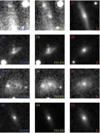
Of the 52 galaxies in our initial list, we exclude one galaxy (number 27) due to its very peculiar shape (to be discussed further in Section4.4). We then fit the other galaxies for all images and for all bands where they are present. Stars (as PSFs) or secondary galaxies (as 1 or 2 component Sersics) within the fitting window (a box 61 pixels on a side for HST) are also fit to take into account their influence on the primary galaxy. Diffraction spikes are fit as Sersics, albeit the resulting fit is very elon-gated. The fit fails in a few cases to obtain a reasonable result; reasons for that are (i) the galaxy is invisible in the image, (ii) the galaxy is too faint compared to other neighboring sources or (iii) image artifacts (usu-ally diffraction spikes). In general, fainter galaxies have more problems and fits fail more often; this is particu-larly problematic in F 606W since our K′-band selected
galaxies are typically fainter in that band. Since faint sources are not constraining astrometrically, that is not a problem.
3.5. Differential Chromatic Refraction
The atmosphere of the earth refracts light:
α = α′tan(ζ) (1)
Therein ζ is the angle from zenith and α′is the deflection
at 45◦. Most of the refraction is corrected for
automat-ically in any linear transformation, see Section4.2 and Fritz et al.(2010), such that it does not impact relative astrometry. It is not possible this way to correct refrac-tion which depends on the color of the source, differen-tial chromatic refraction (DCR). The refraction depends in the following way on λ:
α′= n(λ) 2
− 1
2 n(λ)2 . (2)
Specifically, the effective wavelength of the source within the used band sets the refraction. While DCR is large in the optical (Kaczmarczik et al. 2009; Fritz & Kallivayalil 2015), it is much smaller in the in-frared (Fritz et al. 2010). Of the near inin-frared bands it is smallest in the K-band (Trippe et al. 2010;Fritz et al. 2016). This is one of the reasons why we use K’-band observations. Since essentially all stars (especially the relatively blue Pyxis stars) are in the Rayleigh-Jeans tail in the K’-band the DCR effect between the stars in our observations is less than 0.2 mas even at ζ = 45◦
(Fritz et al. 2010,2016).
In contrast, galaxies have a longer effective wave-length because they are redshifted. We use the cata-log of Galametz et al. (2013) to estimate the observed H − Kscolor of our reference galaxies from the K′
mag-nitudes. We obtain that the mean color is H −Ks= 0.79
(Vega) mag, and that the variation with magnitude is weak. From photometric redshift catalogs, like that of Ilbert et al.(2009), it follows from their magnitudes that our galaxies have a redshift of about z= 0.9. Using red-shifted spectra of galaxies as in Fritz et al. (2016), we obtain that the H − K′ color of such redshifted galaxies
is consistent with the colors in Galametz et al.(2013). We then use redshifted galaxies like inFritz et al.(2016) to obtain that the typical DCR shift between blue stars and galaxies is about 0.5 mas at ζ = 45◦. This shift is
probably overestimated, because the brighter, astromet-rically more important galaxies, are slightly bluer and thus more similar to stars. Pyxis was observed with ζ between 7.2◦ and 20.6◦. Since DCR scales as total
at-mospheric refraction, it follows from Equation1that the the DCR difference is at most 0.17 mas or 0.03 mas yr−1.
On average over the 30 images DCR is even smaller, it is 0.01 mas/yr in Dec. and even smaller in R.A. This is negligible compared to our other errors, especially the reference frame (to be discussed in Section4.4), so we did not attempt to correct it.
3.6. Summary
We derive stellar photometry and astrometry from HST and AO imaging; for the former we use standard routines and for the latter we develop custom PSFs. We evaluate individual sources via visual inspection to classify spurious sources (e.g., cosmic ray hits), stellar sources, and non-point sources; the latter are quantita-tively evaluated using Galfit and determined to be ei-ther unresolved binaries or galaxies. We use 2-d Sersic models to determine the true photocenters of galaxies in both the HST and AO imaging. We use a preliminary distortion correction to refine the locations of the sources for matching across catalogs and evaluate the impact of DCR. At the conclusion of this process, we have velocity measurements for 349 stars and 32 galaxies. That are less objects than detected in K’-band (Section3.2.1) be-cause some are outside of the HST field of view or could not be fit on the HST images due to faintness, com-plex source shape, or a too bright neighboring source or diffraction spike.
4. DERIVING THE PROPER MOTION OF THE
PYXIS CLUSTER
We describe here how we derive the proper motion of Pyxis using HST and GSAOI data. For good proper mo-tions a good distortion correction is necessary. Deriva-tion of the distorDeriva-tion correcDeriva-tion begins with classifying the stars as Pyxis members and non-members. The clas-sification of stars in this way is an iterative process us-ing both photometry and astrometry (Section4.1). This analysis starts with an isochrone analysis. That classifi-cation is then used in the preliminary determination of the distortion and preliminary relative proper motions (Section 4.1). This then leads to a refinement of the membership classification using the preliminary proper motions. This cycle is then repeated until the mem-bership uncertainty found is not an important source of proper motion error. The distortion correction is ex-plained in detail in Section4.2. This Section concludes with deriving position uncertainties and some additional checks for proper motion systematics. Then, we deter-mine the final relative proper motions for the stellar sources, including a full evaluation of the astrometric reference frame (Section4.3). We summarize our error budget in Section 4.5before deriving the final absolute proper motion in Section4.6.
4.1. Pyxis Membership Determination
Our observations contain both Pyxis stars and unas-sociated field stars. The latter are usually foreground stars in the Galactic disk, because there are few stars around the distance of Pyxis in the halo. The target star
selection is important; firstly, because only Pyxis stars should be used for calculating the motion, and secondly, whether stars are members or not is relevant for how they are used in the distortion derivation (Section4.2). Our selection is an iterative process using photometry and astrometry.
We start with photometry. We use the optical HST photometry, because it has higher SNR for the rather blue Pyxis stars. To select members we use the best fit-ting isochrone fromDotter et al.(2011). We obtain this isochrone from the Dartmouth stellar evolution database (Dotter et al. 2008) which was also used byDotter et al. (2011). We determine by hand which offset needs to be added to the isochrone so that it matches the observed Pyxis star sequence. Since the majority of the blue stars are Pyxis members (see Figure 6), the details do not matter much for Pyxis star selection. We obtain offsets of 18.859 magnitudes in F 606W and 18.525 magnitudes in F 814W . This procedure corrects for distance, ex-tinction and imperfect zeropoints. To select Pyxis stars we shift the isochrone slightly. The shift (0.062 mag at bright magnitudes and more at the faint end, see Fig-ure 6) is chosen such that the box contains nearly all stars in the Pyxis sequence.
We then use this first sample for the first run of the distortion correction, which uses only Pyxis stars, see Section4.2. However, we do not use stars brighter than mF814W= 20.7 in the first iteration because bright stars,
which are not Pyxis members, can bias the distortion correction severely. We use then this preliminary dis-tortion correction to calculate the preliminary relative proper motions, using the median position over all detec-tions for the K’-band posidetec-tions, and for HST posidetec-tions, the average of all detections. The error of the proper mo-tions is dominated by the scatter over the K’-detecmo-tions. The error contribution from HST is relatively minor. In two iterations we then exclude stars whose motions di-verge by more then 4σ or 0.4 pixels = 3.9 mas yr−1
from the Pyxis proper motion. That error is dominated by K′-band SNR, therefore it is a function of K-band
magnitude, see Figure 6. Four stars fainter than the limit are excluded with this cut. Of the stars brighter than this limit, three are clearly not members, two are clearly members, and two are borderline cases. We in-clude them in our primary sample but we also check how the proper motion changes when we exclude them. The primary sample consists of 220 Pyxis stars.
As another test of whether our motion is sensitive to the Pyxis selection, we widen the selection box by a factor of three. That adds 18 stars, but 7 of them are astrometrically not Pyxis members. Thus, this variant only includes 11 additional stars, all of which are faint.
Figure 6. Final selection of Pyxis stars, using photometry and astrometry; stars need to fulfill both criteria to be iden-tified as Pyxis Members (blue dots), otherwise they are non-members (red stars). Two are unclear (gray triangles). Top: Color magnitude diagram. The range of color is restricted on the red side, to make the plot in the Pyxis region clearer. The Pyxis isochrone (black) is from the Dartmouth stellar evolution database using the determination byDotter et al.
(2011). The gray lines show the selection box. Bottom: 2D proper motion/2D offset compared to the mean Pyxis mo-tion. The dashed green line shows the typical error as a function of magnitude. The solid black line shows our selec-tion criterion, stars above it are excluded from the sample.
The impact of including these stars is smaller than of using the two bright stars, because these stars are of lower weight in the motion due to their SNR.
Finally we calculate whether the selection of Pyxis stars impacts the velocity of Pyxis. Therefore we repeat the calculation in Section4.4for the different Pyxis star samples. We obtain that the uncertainty in the selection of Pyxis stars adds an error of 0.05 mas yr−1.
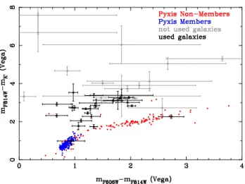
As an additional test, we show here the color-color diagram of all our sources, not just the stars, see Fig-ure7. We use galaxies as reference objects, because due
to tip-tilt star constraints, it is not possible to select a field with a quasar. Also galaxies are less affected by residual distortion, because since we can use several of them, these systematics roughly average out. The galaxies are selected morphologically, see Section3.2.1. For a given F 606W − F 814W color in Figure7, most galaxies are redder than stars in F 814W − K′. This
is expected because galaxies are redshifted compared to the stars. Some galaxies overlap with the stellar se-quence, as it is expected for these and similar colors, see e.g. Galametz et al. (2013). Galaxies that are blue in F 814W − K′ are all obviously extended in our images,
such that it is clear from visual inspection that they are galaxies. In contrast, the more compact galaxies are all outside of the color-color stellar locus, which confirms our visual morphological selection.
We check also the locations of our stellar sources in the color-color diagram. The vast majority lie on the stellar locus and are thus obviously stars. There are two sources which are clearly redder in F 814W − K′ as is
expected for QSOs. We check these sources: one of them lies on a strong diffraction spike in the HST images, making its properties unreliable. The second source has a K′ = 21.6 mag and an absolute proper motion of 4.7
mas yr−1 and we conclude that it is probably a star.
Since the different optical and NIR imaging were not obtained simultaneously, it is also possibly that it is a variable star. Regardless, with a position uncertainty of about 0.5 mas yr−1, the object has a low weight in the
proper motion fitting and is not providing any useful constraints.
4.2. Distortion correction, image registration and position errors
For distortion correction we start with a similar ap-proach as inFritz & Kallivayalil(2015), which assumes that one data set is clearly easier to correct for dis-tortion. For this analysis, HST data is better than the GSAOI data because the distortion of ACS/WFC is well-characterized and stable in time apart from the linear terms (Anderson & King 2006). An STScI-developed code (Anderson & King 2006) was used to perform the geometric distortion correction of the source positions. This leaves offsets induced by the time de-pendence to be removed by a separate linear transfor-mations. After applying this distortion correction we correct for all linear terms, including skew terms, by means of fully general 6-parameter transformations into the F 814W image, which has the largest overlap with the GSAOI imaging.
The distortion of GSAOI is not known for this study, because it is not stable on long time scales (Neichel et al.
Figure 7. Color-color diagram of the observed sources. It is clearly visible that essentially all morphologically-selected stars (dots, error bars are omitted for clarity) share the same sequence, the stellar locus. Galaxies (triangles with error bars) form mostly a cloud above this sequence. The ‘used galaxies’ show the reference sample against which the proper motion of Pyxis is obtained.
2014), thus we must derive the distortion solution em-pirically from our images. Our full distortion correction for GSAOI is a combination of using an external true reference (HST in our case; Section 4.2.1), as well as internal referencing within the GSAOI data itself (Sec-tion4.2.3).
4.2.1. External Distortion Correction for Pyxis using HST
Since the HST data was observed at a different epoch, we can only use objects which have not moved relevantly as an external reference. Unfortunately, there are too few bright galaxies for the distortion correction. The non-Pyxis members of Section4.1are nearly all Galactic disk stars, which are likely to have larger proper motions than our distortion correction can tolerate. In other work,s often the members of the target satellite are used for distortion correction. The member stars in Pyxis have internal motion and thus move relative to each other. This motion could correspond to an additional error term which needs to be added to the other errors terms when a distortion solution is derived (for exam-ple as inDalessandro et al. 2016;Massari et al. 2016a). However, the relative importance of the internal motions can be ascertained from the internal velocity dispersion of Pyxis.
Since no measurement of the dispersion of Pyxis ex-ists, we instead use data from other globular clusters to determine scaling relations for this quantity, using data from Harris(1996). We start with the luminosity, find-ing that faint globular clusters like Pyxis have smaller dispersions. In addition, the dispersion depends on the
mass concentration. We use as a measure for the size of the globular cluster the half light radius. We obtain that, as expected, σ ∝ p(L/rhalf) is valid. Using for
Pyxis MV = −7.0 and rhalf = 17.7 pc (see Section4.6)
we obtain for Pyxis σ = 0.97 ± 0.16 km/s, where the error is from the scatter in the relation over the glob-ular clusters with both measurements. The properties of Pyxis are somewhat uncertain, but it is clear that the dispersion of Pyxis is less than 2 km/s, which trans-lates at its distance into a proper motion dispersion of less than 0.01 mas yr−1. This is negligible compared to
other terms (Section4.2.3and4.5.), and thus we ignore it.
Similar to the approach inFritz & Kallivayalil(2015), we combine the determination of the distortion with the determination of the linear terms, which register the im-age and correct the imim-age scale. For the fitting, we use the mpfit package (Markwardt 2009).
The linear terms can be described as follows, R.A. = c1+ c2xcor+ c3ycor
Dec. = d1+ d2xcor+ d3ycor
(3) and are as expected not stable. This is primarily due to airmass variation, but other effects, such as atmospheric turbulence and corrections made by the the AO system, contribute also to modulations of the image scale.
For the distortion correction, we fit both cubic and quadratic order polynomials finding that the χ2/d.o.f.
of both are quasi-identical. This suggests that the cu-bic approach overfits the data and we therefore adopt a quadratic correction of the form:
xcor= a1+ a2x′+ a3y′+ a4x′2+ a5x′y′+ a6y′2
ycor= b1+ b2x′+ b3y′+ b4x′2+ b5x′y′+ b6y′2
(4) Here the constant and linear terms are used to ac-count for the offsets and scale differences between the four chips. Chip 1 is the reference, thus a2 and b3 are
for chip 1 defined to be 1, and a1, a3, b1 and b2 are
de-fined to be 0. As usual all distortion parameters are different for the four distinct chips. Equation 3 and 4 are also used in Section4.2.3. In practice, we apply first the distortion correction (Equation 4) to the data and then apply the linear terms (Equation3).
We test whether the four detectors should be treated independent of each other for the linear correction (Equation 3), but we find that in this case the er-rors are larger than when we fit these time-dependent linear terms to all four detectors simultaneously. The preference for coupled chips is also supported by fact that the χ2 values are smaller when they are coupled.
parameters is the better strategy: firstly, because the relative chip orientation is effectively stable. Secondly, because there are relatively few bright sources in the images, it is preferable to fit fewer terms.
4.2.2. Tests for Stability over Full Observation Window
We test whether the distortion is stable over the 2.5 hours over which we observed Pyxis (Fritz et al. 2016). Thereby, we solve for different distortion coefficients when the astrometric loop is closed (i.e., within each six-image set), versus considering all the 30 images, i.e., even when the astrometric loop is not closed. This test is done relative to our mosaic since it is then possible to treat all stars, also not Pyxis members, the same way. We find a slight decrease in the error floor in the x-dimension from 0.40 mas (when only one distortion so-lution is derived for all the 30 images) to 0.29 mas (when one distortion solution is derived for only the images in the closed loop) to 0.24 mas (when different distortion solutions are derived for each of the 30 images), and in the y-dimension from 0.26 mas to 0.24 mas to 0.22 mas, for the three cases respectively. Stated differently, we find a relatively small decrease in the error floor of 0.16 mas in x and 0.02 mas in y. While some improvement is expected when allowing these terms to vary (because the GeMS/GSAOI system is not stable; see discussions in Neichel et al. 2014) and/or (because of atmospheric variability; see discussions inMassari et al. 2016b), it is surprising that the error floor decreases when all images are used versus when the astrometric loop is closed since during this time the distortion should be stable. There-fore, the improvement is probably caused by more de-grees of freedom. Further, the decrease of the error floor is small when compared to other errors. We therefore assume the distortion solution is stable over the total observation window for the analyses to follow.
4.2.3. Internal Distortion Correction
It turns out that the Pyxis member-star sample does not obtain a sufficiently good distortion correction solu-tion, due to the fact that the system is relatively sparse, and we find that when using only this sparse sample, the resulting offset between chips has a non-negligible uncer-tainty. The bulk of the Pyxis member-star sample has lower SNR (i.e., the bulk of the Pyxis stars are faint), while non-member stars are typically brighter. Thus we devise a method to leverage these brighter stars in the distortion solution. Since the non-members move, we cannot use their position on the HST image as refer-ence. We must instead use their positions only within the GSAOI data which was all taken within the same epoch. We use the first GSAOI image as reference, be-cause i) it is in the center of all images and thus has the
biggest overlap with the other images, and ii) this image has also a relatively high Strehl ratio compared to the other images in the program. Since, the first GSAOI im-age is distorted as well, we also have to apply the same distortion correction to the positions in the first image, as described further below. This procedure adds 170 stars that we can use to help bootstrap the distortion terms. Overall, we end up using 390 of the 450 stars for deriving the distortion correction (5 stars are omitted because they are saturated or close to a saturated star in the first image and an additional 55 stars are excluded because they are not on the first image).
We can no longer use mpfit for this expanded sam-ple, because for non-Pyxis members there are no true positions which remain unchanged between frames (i.e., the non-Pyxis stars have no known position, since they depend on the distortion which is yet to be determined). We instead develop our own Monte Carlo fitting method. As a starting point we use the distortion solution de-rived using only Pyxis stars. Because the fitted function contains 222 free parameters, the minimum cannot be reached in a sufficient time if all are allowed to remain free. After some initial iterations, we fix all parame-ters that affect only one image in the solution; these include all linear parameters to transform each individ-ual GSAOI image to HST, with the exclusion of the parameters of the first GSAOI image, which is used as the ‘reference’ image for all non-Pyxis stars. It is ex-pected that the influence of these parameters is reduced by√N since N (up to 29) different images are used to calculate the final positions. After fixing these frame-specific parameters, the 48 parameters are left to vary in the fit, which increases the speed of the procedure.
As a result of our custom Monte Carlo fitting proce-dure, the uncertainties for the fitted parameters in the distortion solution (e.g., the chip separations) are now small compared to the positional errors of the galax-ies used to define the absolute frame. The impact of imperfect linear terms in the distortion solution (those held partly fixed in the fitting process) is included de facto for galaxy positions, because the total uncertainty in the position of an individual source is derived from its frame-to-frame scatter. The two PSF options (PSF1 and PSF2) obtain consistent proper motions.
4.2.4. Position Errors
Here we describe more fully the initial set-up and re-jection criteria used for the Monte Carlo method above, and then give an estimate of the typical position errors that we achieve after distortion correction. For an ini-tial set of input errors for the stars, we use the Galfit positional uncertainties. In the first iteration, we
iden-tify the Pyxis members (Section 4.1). Since the Pyxis membership of a few stars is uncertain, we use two dif-ferent samples, which include the uncertain stars or not. We also test positions obtained with both of our model PSFs. We then proceed with each possible combination of PSF and Pyxis membership sample.
We first clean each sample of outliers based on a com-parison to its median position, defining a cutoff criterion as follows:
Ri=
q
∆Rx, i2+ ∆Ry, i2< η σi, (5)
where ∆Rx, i and ∆Ry, i are the differences between the
median position of the source and its position in the i-th image, σi is the positional scatter of this star and η
is a scaling factor that is changed iteratively. The be-havior of the solution is monitored with stricter cuts on η and, in our final iteration, we use η = 5. Then we measure the scatter over all detections of a star (i.e., in all the images for which it has a good detection). We also calculate 1.483× the median deviation of the stellar positions as a robust measure of the positional scatter, and adopt a ratio between the scatter and this median to adjust the final uncertainty for each source. How-ever, sometimes low number statistics can cause non-physically small scatter values, and to safeguard against this, we also keep track of the typical error expected for stars of a given magnitude (as coded basically by their SNR and quality of fit to the PSF), and use this typical value if it is higher than the scatter.
We modify the process slightly for non-Pyxis stars. Already in our first iteration we include an error floor estimate, because for some bright stars the uncertainty scaled by the SNR is much smaller than realistic er-rors. In a second iteration, we then exclude outliers with Ri > 5σi and again adjust uncertainty using the scatter
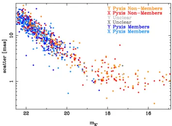
as before. To avoid any single star having a very large weight in the final fit, we set a minimum uncertainty of 0.5 mas. This is somewhat smaller than our error floor (≈ 1 mas) measured after the final iterations, see Fig-ure8. This floor is mainly caused by residual distortion, and its level is consistent with other measurements for GSAOI, seeNeichel et al. (2014).
We now present the typical positional errors we obtain after the distortion correction process is done. In sub-sequent analysis, we use the median position of a star in the GSAOI images, after application of the distortion correction, as the star’s final position for the GSAOI epoch. The uncertainty in this position is defined as the robust scatter of the set of frame positions divided by the square root of the number of images in which the source appears. Because the distortion residuals probably do not average out over the small (1′′) dither between
in-Figure 8. GSAOI position scatter of the stars used in the transformation. Dots stand for the scatter in X (the X of the HST image), boxes for the scatter in Y. We use 1.483· the median deviation as a robust scatter measure. The scatter is measured after transformation into the HST reference frame, thus it contains also a contribution from residual distortion. Only the scatter for PSF1 is shown, but the difference be-tween PSF1 and PSF2 is small.
dividual frames, but do average out over the large (7′′)
dither between image sets, we add an additional error term of 1 mas (the error floor) divided by the square root of the number of image sets in which the source appears (maximum of 5). This estimate is conservative since there are fewer large dither steps (5) than there are images (30). In the best case, bright stars detected in 5 images sets, we obtain a precision of 0.4 mas in the star positions and of 0.08 mas yr−1 in the proper
motions. The final uncertainties for star positions only affect the relative motions; for the absolute motions, the error contribution of the reference galaxies is the domi-nant term.
4.2.5. Comparison to Other GSAOI Distortion Solutions
We now analyze and compare our distortion field with those previously found in the literature. The maximum distortion vector of our distortion field is 12.9 pixel, which is 259 mas. To ease comparison with most lit-erature, we set the average shift in our distortion map to zero by a linear transformation in the same way as Ammons et al.(2016). We show the derived distortion map in Figure 9. The standard deviation over the dis-tortion field is 63 mas in x and 1.8 mas in y. A stronger distortion in x and a similar distortion field was also observed by Ammons et al. (2016) and Massari et al. (2016a) for GSAOI.
We compare our distortion field quantitatively with Ammons et al. (2016)8 and Dalessandro et al. (2016)
(we applied on their field a linear transformation in the same way as to our data). After the transformation, the distortion field ofDalessandro et al.(2016) is similar to the others and shows much larger shifts in x. We cal-culate the difference in the distortion field between us and the Ammons/Dalessandro field. This difference has similar distortion strengths in x and y, the scatter is in both about 4 mas forAmmons et al.(2016) and 3.5 mas for Dalessandro et al. (2016). This difference is much smaller than the distortion in x, but it is clearly bigger than the errors in our and the other distortion determi-nations. The data used for the Ammons et al. (2016) distortion determination was obtained at the end of 2012, and the data of theDalessandro et al.(2016) dis-tortion determination was obtained around May 2013, both well before our observations. Thus, it is not sur-prising that the distortion fields differ, as it is known that the distortion of GSAOI is not stable on long time scales (Neichel et al. 2014). The distortion also depends to some extent on the guide-star asterism used.
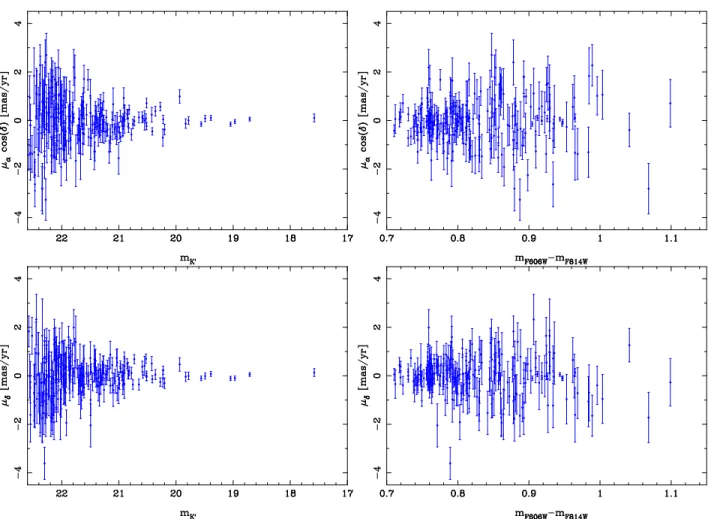
As additional checks for systematics we test, simi-larly to Bellini et al. (2014); Casetti-Dinescu & Girard (2016), whether the proper motion varies as a function of magnitude and color, see Figure 10. We use only Pyxis stars since the other stars have large peculiar mo-tions such that this would hide any trend. It is clear that there is no trend as a function of magnitude or color.
4.3. Relative proper motions of stars
The positions and motions are first measured in pixel space. To transform them into the world coordinate system (WCS), we again utilize the VISTA-VHS data (McMahon et al. 2013) obtained in April 2012, which is astrometrically tied to 2MASS. As before, we only use stars that are isolated in the VHS data. A total of 23 stars are common to the VISTA-VHS observations and our HST footprint. We perform a fit to determine a linear transformation between final pixel positions and the VISTA-VHS WCS. The scatter between transformed HST positions and the VHS positions is 26/25 mas in R.A./Dec9. The positional uncertainty in the
VISTA-VHS WCS must also be considered and this is about 100 mas10. The precise error in the WCS is not important
8
For quantitative use of theAmmons et al.(2016) field we use their distortion parameters directly, which were kindly provided to us.
9
Here, as always, the position/velocity in R.A. is multiplied by cos(Dec.)
10
For details see: https://www.eso.org/sci/observing/phase3/ data releases/vhs dr2.pdf
Figure 9. Distortion map of GSAOI derived from PSF1 data (but the difference is very small between the two PSFs). The vectors showing the distortion field are magnified by a factor of 25. Not shown are linear scale differences and tilts between the different chips. Also the chips do not exactly have the shown positions. Further, a linear transformation which sets the average shift of each chip to zero is applied for easy comparison with the literature.
for us since we are not interested in absolute astrometry, only in absolute motions.
We compute the average motion of the 23 VISTA-VHS stars relative to Pyxis member stars finding it to be ∼16 mas. This difference does not impact our proper motion because we use the same WCS transformation on both the HST and GSAOI epochs. The position uncertainty in the VISTA-VHS frame causes an uncertainty in the overall image scale, which is a systematic uncertainty on the final proper motion. Since the sources used for the WCS transformation extend over 96/56′′in R.A./Dec.,
the image scale uncertainty is at most 0.11/0.17% using the 100 mas error in the VISTA-VHS WCS. Without accounting for this error term, the motion uncertainty is 0.86% of the motion for the stars with the smallest fractional motion uncertainty. Thus, even in the most extreme case, the image scale error is smaller than the other error components (even more so for the absolute proper motion, see Section4.4).
As test we calculate the error weighted average motion of the Pyxis members. We obtain
µαcos δ = −0.04 ± 0.02 mas yr−1 and µδ = 0.01 ± 0.02
mas yr−1. Given that Pyxis is the reference the motion