Current and Future Arctic Aerosols and Ozone From Remote Emissions and Emerging Local Sources—Modeled Source Contributions and Radiative Effects

HAL Id: hal-02292757

https://hal.sorbonne-universite.fr/hal-02292757

HAL is a multi-disciplinary open access

archive for the deposit and dissemination of sci-entific research documents, whether they are pub-lished or not. The documents may come from

L’archive ouverte pluridisciplinaire HAL, est destinée au dépôt et à la diffusion de documents scientifiques de niveau recherche, publiés ou non, émanant des établissements d’enseignement et de

Current and Future Arctic Aerosols and Ozone From

Remote Emissions and Emerging Local Sources-Modeled

Source Contributions and Radiative Effects

Louis Marelle, Jean-Christophe Raut, Kathy S. Law, Olivier Duclaux

To cite this version:

Louis Marelle, Jean-Christophe Raut, Kathy S. Law, Olivier Duclaux. Current and Future Arctic Aerosols and Ozone From Remote Emissions and Emerging Local Sources-Modeled Source Contribu-tions and Radiative Effects. Journal of Geophysical Research: Atmospheres, American Geophysical Union, 2018, 123 (22), pp.12,942-12,963. �10.1029/2018JD028863�. �hal-02292757�

See discussions, stats, and author profiles for this publication at: https://www.researchgate.net/publication/328566016

Current and Future Arctic Aerosols and Ozone From Remote Emissions and

Emerging Local Sources—Modeled Source Contributions and Radiative Effects

Article · October 2018 DOI: 10.1029/2018JD028863 CITATIONS 0 READS 46 4 authors, including:

Some of the authors of this publication are also working on these related projects:

VOC oxydationView project

PM characterisation and modelingView project Louis Marelle

IGE / LATMOS

30 PUBLICATIONS   191 CITATIONS    SEE PROFILE

Jean-Christophe Raut

Sorbonne University, Paris, France

121 PUBLICATIONS   1,846 CITATIONS    SEE PROFILE

Olivier Duclaux

TOTAL Solaize France

23 PUBLICATIONS   75 CITATIONS    SEE PROFILE

Current and future Arctic aerosols and ozone from

remote emissions and emerging local sources

-modeled source contributions and radiative effects

Louis Marelle, [email protected]

1_{LATMOS/IPSL, Sorbonne Universit´e,}

UVSQ, CNRS, Paris, France

2_{TOTAL S.A, Direction Scientifique, Tour}

Michelet, 92069 Paris La Defense, France

3_{CRES, Centre de Recherche TOTAL,}

69360 Solaize, France

This article has been accepted for publication and undergone full peer review but has not been through the copyediting, typesetting, pagination and proofreading process, which may lead to differences be-tween this version and the Version of Record. Please cite this article as doi: 10.1029/2018JD028863

Abstract. The Arctic is influenced by air pollution transported from lower latitudes, and increasingly by local sources such as shipping and resource ex-traction. Local Arctic emissions could increase significantly in the future due to industrialization in a warming Arctic, and further influence Arctic climate. We use the regional model WRF-Chem to investigate current (2012) and fu-ture (2050) sources of Arctic aerosol and ozone pollution and their radiative impacts, focusing on spring and summer emissions from mid-latitude anthro-pogenic sources, biomass burning, Arctic shipping, and Arctic gas flaring. Results show that remote anthropogenic and biomass burning emissions are likely to remain the main source of Arctic pollution burdens and of black car-bon (BC) deposition over snow, and the main contributors to direct aerosol and ozone radiative effects in the Arctic. However, local Arctic flaring emis-sions are already a major source of BC in Northwestern Russia, with a

di-rect radiative effect of ∼ 25 mW m−2, and Arctic shipping is a strong

cur-rent source of aerosols and ozone during summer in the Nordic Seas. We find that the direct effect of ozone and aerosols from summertime Arctic ship-ping are respectively negative (due to frequent temperature inversions) and positive (because of the high surface albedo) in our simulations, two new re-sults. With the development of diversion shipping through the Arctic Ocean in summer 2050, Arctic shipping emissions could become the main source of surface aerosol and ozone pollution at the surface, with strong associated

indirect effects of −0.8 W m−2, while flaring would remain an important BC

Keypoints:

• Significant contributions from Arctic shipping and gas flaring to present-day and future surface Arctic pollution

• Ozone from shipping cools the atmosphere due to the near-surface tem-perature inversions in the Arctic

• Significant negative summertime aerosol indirect effects (−0.8 W m−2₎

1. Introduction

The Arctic atmosphere is influenced by air pollution transported from lower latitudes. Anthropogenic emissions from Europe, Asia and North America in the midlatitudes are currently the main source of Arctic pollution, especially in winter and spring when pole-ward atmospheric transport is efficient and removal processes are weak [Barrie, 1986; Stohl , 2006]. Biomass burning at middle and high latitudes is also an important source of Arctic pollution during late spring and summer [Brock et al., 1989; Stohl , 2006; Warneke et al., 2009; Ikeda et al., 2017], although its exact contribution is uncertain. These remote emissions are an important source of Arctic aerosols (e.g. black carbon (BC), sulfate) and ozone, which act as short-lived climate forcers that can enhance or mitigate the observed rapid Arctic warming [Shindell et al., 2006; Najafi et al., 2015; AMAP , 2015]. Ozone is a greenhouse gas, and also absorbs short wave radiation directly [e.g., Berntsen et al.,

1997]. Aerosols can scatter or absorb short wave radiation [direct effects, ˚Angstr¨om, 1929;

Haywood and Shine, 1995]; influence the life cycle of clouds by modifying atmospheric tem-perature and humidity profiles [semi-direct effects, Hansen et al., 1997]; and influence cloud formation, cloud optical properties, cloud height and cloud lifetime through their microphysical interactions with cloud droplets [indirect effects, Twomey, 1977; Albrecht , 1989]. In addition, absorbing aerosols deposited on snow reduce the surface albedo and lead to earlier snow melt [Warren and Wiscombe, 1980].

Decreasing anthropogenic emissions in Europe, Western Asia and North America are thought to be responsible for the observed decline in black carbon and sulfate aerosol concentrations at several surface sites in the Arctic [Hirdman et al., 2010; Sharma et al.,

2013], and these declining trends could continue in the future due to further global re-ductions in emissions of short-lived climate forcers and their precursors [IPCC , 2013]. At the same time, Arctic warming and the associated decline in sea ice [Kirtman et al., 2013] is progressively opening the region to human activity, especially shipping and resource extraction [IPCC , 2014]. Local Arctic pollutant emissions could increase rapidly as a result [Corbett et al., 2010; Peters et al., 2011]. It is currently unclear if local Arctic emis-sions could then start to have a more significant impact on Arctic air pollution, compared to the historically predominant remote sources, and whether local sources could become important drivers of Arctic climate change or have an impact on regional air quality or ecosystems [Arnold et al., 2016; Law et al., 2017]. These questions are important for pol-icymakers, who need to understand the trade-offs between air quality and climate when reducing local Arctic emissions of short-lived pollutants and their precursors [Schmale et al., 2014; Stohl et al., 2015; Sand et al., 2016; AMAP , 2015].

However, the answer to these questions is currently unclear, for two main reasons. First, models struggle to represent short-lived pollutants, especially aerosols, in the Arctic [e.g., Koch et al., 2009; Eckhardt et al., 2015; Schwarz et al., 2017], due to limited model resolution [Sato et al., 2016; Raut et al., 2017], uncertainties in emissions [Stohl et al., 2013] and uncertainties in processes such as aerosol removal by precipitation and clouds [e.g., Browse et al., 2012; Mahmood et al., 2016; Qi et al., 2017a; Raut et al., 2017]. Second, the lack of accurate emission inventories also makes it difficult to quantify precisely the impact of local Arctic emission sources. Early inventories by Peters et al. [2011] for Arctic oil and gas extraction, and Corbett et al. [2010] for Arctic shipping, used in earlier studies [e.g., Ødemark et al., 2012; Dalsøren et al., 2013; Browse et al., 2013], appear to have

underestimated the magnitude of Arctic pollutant emissions, compared to more recent estimates [Winther et al., 2014; Klimont et al., 2016]. New Arctic emission inventories for flaring associated with oil and gas extraction have already been used in recent studies, highlighting the important contribution from this source to current BC concentrations and BC deposition in the Arctic [Stohl et al., 2013; Xu et al., 2017; Qi et al., 2017a], but with little focus on its potential future impacts.

While global climate models are the ideal tools for estimating future radiative impacts of short-lived and long-lived climate forcers, they often include simplified representations of chemical and aerosol processes including aerosol-cloud interactions [e.g., see Sand et al., 2017]. In addition, the resolutions of global model used to study Arctic aerosols and

ozone remain low, typically 2°×2° or lower for coupled chemistry-aerosol-climate models

[Eckhardt et al., 2015; Emmons et al., 2015]. Alternatively, regional models only simulate limited domains, which costs less computing power than simulating global domains, freeing computing resources in order to either increase the resolution, use more complex physics, aerosols, or chemistry schemes, or in order to run longer simulations or ensembles to quantify the statistical significance of model results

In this study, we use the regional model WRF-Chem 3.5.1 [Weather Research and Forecasting model, including chemistry; Grell et al., 2005; Fast et al., 2006], which includes explicit calculations of the aerosol size distributions within 16 size bins (8 interstitial and 8 in clouds) for sulfate, nitrate, ammonium, primary and secondary OA, BC, dust and sea salt, as well explicit aerosol activation in clouds and “online” feedback on the meteorology, allowing us to calculate the indirect effect of aerosols directly [details are given in Section 2 and in Marelle et al., 2017]. To our knowledge, the only model included

with similar capabilities in the Arctic intercomparisons of Eckhardt et al. [2015] or in the assessment report of AMAP [2015] is CESM1-CAM5. However, CESM1-CAM5 uses fewer parameters for the size distribution, does not include nitrate aerosols, and was run

in these studies with a low resolution of 1.9°×2.5° and 30 levels. The WRF-Chem model

has recently been improved for the Arctic and is now able to capture observed aerosols and ozone in the Arctic [Marelle et al., 2017, details in Section 2.3]. It is run here with recent inventories for current (2012) and future (2050) remote and local Arctic emissions [Winther et al., 2014; Klimont et al., 2016].

In Section 2, we present the WRF-Chem model, the emission inventories, and the dif-ferent simulations performed in this study. These simulations are used to compare the relative influences of local (Arctic shipping and gas flaring) and remote (midlatitude an-thropogenic emissions, biomass burning) sources of Arctic aerosols and ozone, on surface aerosol concentrations, surface ozone concentrations, and black carbon deposition in the Arctic (Section 3); on the vertical distribution of aerosols and ozone in the Arctic (Sec-tion 4); and on the direct and indirect radiative effects of aerosols and ozone in the Arctic (Section 5). Conclusions are presented in Section 6. The focus of this study is to inves-tigate the effect of emissions from these different sources in the present-day and in the future. For this reason, we change emissions but keep the meteorological conditions the same in the present-day and future simulations.

2. Methods

The impacts of the different emission sources are determined by performing 6-month long (March to August), quasi-hemispheric WRF-Chem 3.5.1 simulations over the Arc-tic, using emissions for the years 2012 and 2050. The WRF-Chem model is a coupled

meteorology-atmospheric chemistry-aerosol mesoscale model based on the model WRF-ARW [Advanced Research WRF; Skamarock et al., 2008]. In this study, we use a version of WRF-Chem 3.5.1 modified for quasi-hemispheric Arctic simulations [Marelle et al., 2017], including updates to the treatment of surface temperatures over sea ice, trace gas de-position and photolysis over snow, dimethylsulfide (DMS) emissions and DMS gas-phase chemistry, aerosol sedimentation aloft, and also including the effects of sub-grid scale clouds on aerosols and trace gases. The Arctic region is defined in this study as the region

from 60° N to 90° N.

2.1. Simulation domain and model setup

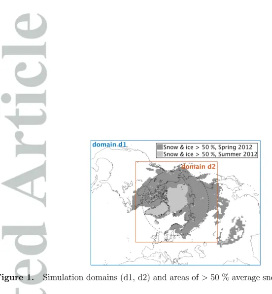
The simulation domains (polar stereographic projection) are shown in Figure 1. The d1 domain includes regions with emissions potentially transported to the Arctic in under 30 days [Stohl , 2006], and the inner d2 domain is focused on the Arctic region. The horizon-tal resolution is 100 km×100 km, with 50 vertical levels. This resolution is similar to the resolution of state-of-the-art global climate models, although coupled aerosol-chemistry-climate global models included in recent intercomparisons in the Arctic [Eckhardt et al.,

2015; AMAP , 2015] used even lower resolutions of 2°×2° or 3°×3° and 30 vertical

lev-els. We used this relatively low resolution in order to use complex physics and aerosol schemes within WRF-Chem, especialy a 2-moment cloud microphysics scheme with ex-plicit aerosol activation and its feedback on cloud properties, and to add additional en-semble simulations. These choices were made in order to calculate indirect effects due to cloud/aerosol interactions directly within WRF-Chem, without using a parameterization for cloud droplet numbers, and also to assess the statistical significance of our results and separate signal from noise, especially for radiative calculations (Section 2.3). We also note

that although there are some models in Eckhardt et al. [2015] with comparable or higher resolutions than in the present study, they are “offline” Lagrangian or chemical-transport models unable to calculate the feedbacks of aerosols and chemistry on the meteorology.

The model setup for meteorology, aerosols and chemistry is presented in Marelle et al. [2017]. Briefly, gas-phase chemistry calculations use the SAPRC-99 [Statewide Air Pol-lution Research Center, 1999 version; Carter , 2000] mechanism, combined to a version of the 8-bin sectional aerosol scheme MOSAIC [Model for Simulating Aerosol Interactions and Chemistry; Zaveri et al., 2008], which includes secondary organic aerosol (SOA) for-mation [Shrivastava et al., 2011], and aqueous chemistry in grid-scale [Morrison et al., 2009] and sub-grid scale [Berg et al., 2015] clouds. Wet removal of BC in WRF-Chem is performed by explicitly calculating activation in clouds of the BC-containing internally mixed aerosols, based on their size distribution and chemical composition and subsequent removal by precipitation. In addition, wet removal by impaction is also calculated. Ra-diative calculations for the longwave (LW) and shortwave (SW) fluxes are performed by RRTMG [Rapid Radiative Transfer Model for Global applications; Iacono et al., 2008], and take into account the effect on radiative transfer of model predicted aerosols and ozone. Initial and boundary meteorological conditions for meteorology, as well as sea sur-face temperatures and sea ice, are from NCEP FNL (National Center for Environmental Prediction, final analysis). WRF winds and temperatures are nudged (grid nudging) to FNL above the boundary layer. Boundary and initial conditions for aerosols and trace gases (domain d1) are from the global model MOZART-4 [Model for Ozone and Related chemical Tracers, version 4; Emmons et al., 2010]. MOZART-4 and FNL fields are up-dated every 6 hours.

The model is run from 15 February 2012 to 1 September 2012, using anthropogenic emissions for 2012 and 2050 (described in Section 2.2). The first 15 days of simulation (15 February 2012 to 29 February 2012) are considered as spin-up and are discarded from the analysis. Model results are thus available for two seasons, spring (March-April-May, MAM), when long-range pollution transport to the Arctic is significant, and summer (June-July-August, JJA), when long-range transport is less efficient, loss by wet deposition more prevalent, and when local emissions could play a larger role, especially shipping due to ice-free conditions. This limited 6-month period is thus well-adapted to reach one of the main objectives of this study, which is to compare the impacts of emerging local Arctic sources and of the more well-known remote sources. It is also the period when the direct radiative effects of Arctic aerosols are the largest [Sand et al., 2017].

In this study, we focus on quantifying relative contributions from different anthropogenic emission sources in the present day (2012) and in the future (2050). Therefore, simulations for 2050 are also forced by 2012 sea ice, sea surface temperatures, and meteorology from the NCEP FNL analysis, and use present-day vegetation, as well as 2012 chemical, initial, and boundary conditions from the MOZART-4 model. For tropospheric ozone, we focus

on the contribution of non-methane precursor emissions of nitrogen oxides (NO_x), volatile

organic compounds (VOCs) and carbon monoxide (CO), in line with previous analyses (AMAP, 2015). Methane concentrations are not directly calculated in WRF-Chem 3.5.1 and are set to a constant level throughout the troposphere [1.893 ppm in this study; Blasing, 2014] in the 2012 and 2050 simulations. Longer simulations would be needed to quantify the contribution from methane oxidation and effects related to methane feedbacks on tropospheric ozone.

2.2. Emissions

Anthropogenic emissions are taken from the ECLIPSEv5 inventory [Evaluating the Cli-mate and Air Quality Impacts of Short-Lived Pollutants; Klimont et al., 2016], except sub-Arctic shipping emissions from RCP8.5 [Representative Concentration Pathway 8.5; Riahi et al., 2011] and Arctic shipping emissions from Winther et al. [2014]. Biomass burn-ing emissions for 2012, includburn-ing wildfires and agricultural burnburn-ing, are from FINNv1.5 [Fire INventory from NCAR, version 1.5; Wiedinmyer et al., 2014]. In order to avoid double-counting, agricultural fire emissions from ECLIPSEv5 are not used. Emissions of terrestrial biogenic compounds, sea salt, dimethylsulfide (DMS), mineral dust, and

lightning NO_x are calculated online by the model, as described in Marelle et al. [2017].

Future anthropogenic emissions in 2050 follow the ”Current legislation” (CLE) scenario for ECLIPSEv5, assuming full enforcement of current and planned environmental regu-lations. As a result, between 2012 and 2050, ECLIPSEv5 March to August emissions of

NO_x, SO₂ and BC within the d1 domain change by +24 %, +27 % and −27 %. In this

study the focus is on the changes in anthropogenic emissions. For this reason, wildfire emissions and agricultural burning, collectively denoted as biomass burning, as well as natural emissions, are the same in the 2012 and 2050 simulations. In addition, initial and boundary conditions (as well as emissions within MOZART-4 driving these) do not change between the 2012 and 2050 scenarios

Local emissions from flaring associated with oil and gas extraction, primarily in north-ern Russia, are included as part of the ECLIPSEv5 dataset, and local Arctic shipping emissions are from the inventory of Winther et al. [2014]. In 2050, additional “diversion shipping” emissions from Corbett et al. [2010] are used, corresponding to a diversion of 5%

of global shipping through the Arctic Ocean. We assume that Arctic diversion shipping occurs in July and August, following Corbett et al. [2010], and that diversion shipping emissions are equally divided between the Northern Sea Route and the Northwest Pas-sage. All future shipping emissions are based on “High Growth” projections, described

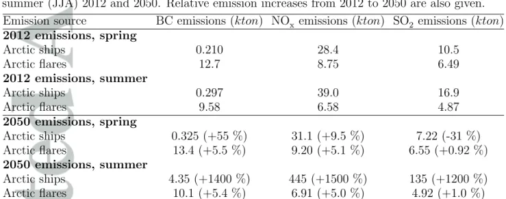
in Corbett et al. [2010] and Winther et al. [2014]. Emission totals of NO_x, SO₂ and BC

from Arctic shipping and Arctic flaring in 2012 and 2050 are given in Table 1. Arctic

shipping mostly emits NO_x and SO₂, and flaring is an important local source of BC [as

already noted by Stohl et al., 2013]. Table 1 shows that flaring emissions from ECLIPSEv5 are relatively stable between 2012 and 2050 [in agreement with earlier findings by Peters

et al., 2011], but that shipping emissions of BC, NO_x and SO₂ from Corbett et al. [2010]

and Winther et al. [2014] increase very strongly in summer 2050 due to diversion shipping

through the Arctic Ocean. Arctic shipping SO₂ emissions (north of 60° N) decrease by

−31% in spring 2050 due to shipping emission controls reducing sulphur fuel contents [IMO , 2010], but, in summer 2050, this decrease in emission factors is more than

com-pensated for by the projected increase in traffic, and total Arctic shipping SO₂ emissions

increase.

2.3. Simulations

The simulations performed in this study are presented in Table 2. The CONTROL sim-ulation includes all sources of emissions. We also perform sensitivity simsim-ulations without emissions from Arctic ships (NOSHIPS), Arctic flares (NOFLARES), mid-latitude

anthro-pogenic emissions south of 60° N (NOANTHRO MIDLAT, including ships) and biomass

These control and sensitivity simulations are performed with 2012 and 2050 emissions (but NOFIRES uses the same biomass burning emissions for 2012 and 2050).

A simulation for the year 2008 using the same setup as CONTROL (on domain d1) was presented and validated against surface and airborne measurements in Marelle et al. [2017], showing good agreement with observed Arctic BC and sulfate. The root mean square error (RMSE) at the Arctic surface in spring and summer 2008 was found to be

14.2 ng m−3 for BC, and 0.261 µg m−3 for sulfate, and the corresponding correlation

coefficients 0.87 for BC and 0.73 for sulfate. WRF-Chem was however shown to be biased high for surface ozone (RMSE 7.56 ppbv), despite a good correlation coefficient of 0.73. This high bias was due to ozone overestimations over sea ice during spring, due to the lack of halogen chemistry in the model. This has only limited impacts on the attribution results presented in this study, since we show in Section 4 that only one source (remote anthropogenic emissions) has significant impacts on ozone in the Arctic lower troposphere during spring. In addition, the radiative effect of Arctic ozone is not very sensitive to concentrations in the boundary layer [Rap et al., 2015].

Sensitivity simulations NOANTHRO MIDLAT, NOFIRES, NOSHIPS and NOFLARES are used to evaluate the impacts of a given emission source on modeled quantities, e.g. CONTROL(2012) - NOSHIPS(2012), to assess the effect of Arctic shipping emissions in 2012. In Sections 3, 4 and 5, results are shown in terms of relative contributions, e.g., [CONTROL(2012) - NOSHIPS(2012)] / CONTROL(2012). Since we do not study every potential source and since non-linearities might be present in the model, the sum of contributions may not add up to 100 %. This is especially the case for ozone, since large natural sources (stratospheric, lightning) are excluded from our analysis. In addition, the

ozone response from switching off sources completely may not be additive, because ozone chemistry is highly non-linear [Wu et al., 2009].

Since emissions from Arctic shipping and flaring activities are only 0.2 % and 0.7 %

of total NO_x and BC anthropogenic and fire emissions in the d1 domain, they may only

have relatively small effects on pollutant concentrations, BC deposition, or on the radia-tive budget in the Arctic. As a result, such effects may be locally small compared to the effects of internal meteorological variability in the model [e.g., Stofferahn and Boybeyi , 2017], making them difficult to quantify. Therefore, in order to separate the signal from these local Arctic emissions from internal variability, we use a filtering approach based on ensemble runs and the Student t-test [Stofferahn and Boybeyi , 2017]. A first CON-TROL simulation is performed on domain d1, and used to set the boundary conditions for the sensitivity simulations NOSHIPS, NOFLARES and a second CONTROL performed on domain d2. Four ensemble members are then generated for each of these runs by initializing the model at 00 UTC, 06 UTC, 12 UTC and 18 UTC on 15 February. A two-tailed Student t-test is later used to assess whether the average effect of, for example, Arctic shipping (ensemble average for CONTROL - NOSHIPS) is different at the 95 % significance level from the variability between the 4 different (in this case CONTROL - NOSHIPS) realizations. This filtering is not used for the NOANTHRO MIDLAT and NOFIRE simulations because of the high computational cost of performing ensembles on the large d1 domain, and because emission changes associated with these sources are large and thus less sensitive to internal variability (see discussions in Sections 3, 4 and 5).

3. Local and remote contributions to surface concentrations and BC deposition in the Arctic

This Section examines the impacts of the different emission sources (anthropogenic activity in the mid-latitudes, biomass burning, Arctic shipping, and Arctic oil and gas flaring) on ozone mixing ratios and aerosol concentrations (excluding dust and sea salt) at the surface (0 to 50 m altitude), and their impacts on BC deposition fluxes in the Arctic. Since local emissions are directly emitted at the Arctic surface, their impacts are expected to be higher at low altitudes. The vertical distributions of these contributions are discussed in the next section.

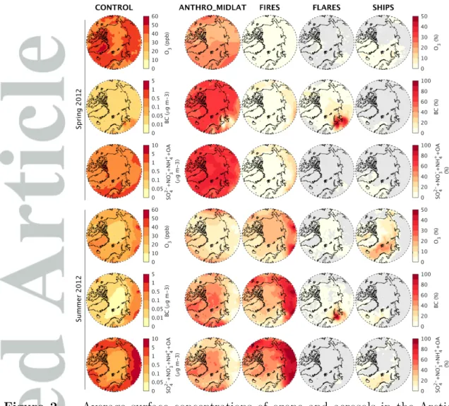
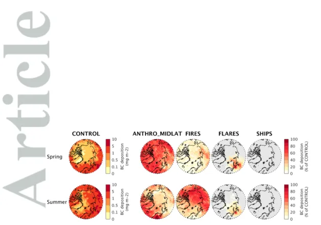
Figure 2 shows the simulated ozone and aerosol (BC; sum of sulfate + ammonium + nitrate + organic aerosol (OA)) surface concentrations in spring and summer 2012, and the contributions from each source. Similarly, Figure 3 presents the contributions from each source to BC deposition in the Arctic. For reasons noted earlier, individual contributions do not necessarily add up to 100 %. In addition, we do not quantify the contributions from local Arctic emissions other than ships and flares or from sources outside of the d1 domain.

In Figure 2, results from the CONTROL simulation (left-hand column) are in agreement with the well-known seasonal cycle of pollution in the remote Arctic [Quinn et al., 2007], increasing in winter and spring and lower during summer. These lower concentrations

in summer are clear at higher latitudes (north of 70° N), but at lower latitudes, aerosol

concentrations increase over land during summer due to boreal biomass burning emissions.

3.1. Present-day (2012) surface concentrations and BC deposition from remote and local emissions

In spring 2012, mid-latitude anthropogenic emissions are an important source of Arc-tic surface ozone (15 to 30 % of total ozone) and aerosols (∼ 70 % of total sul-fate+nitrate+ammonium+OA), and of BC deposition at the surface (∼ 60 %, Figure 3). Biomass burning is a weak source of surface BC in spring 2012, but has a large effect on BC deposition (up to 50 % in Russia). Earlier studies have shown that agricultural fires in Eurasia could be effectively transported to the Arctic at low altitudes in spring during specific events [Stohl et al., 2007; Warneke et al., 2009; Marelle et al., 2015], but this does not seem to occur significantly in spring 2012. During summer 2012, when boreal wild-fires occur, biomass burning emissions are a major source of short-lived pollutants at the surface (15 to 50 % for ozone, 50 to 100 % for BC and sulfate+nitrate+ammonium+OA) and of deposited BC in the Arctic (up to 80 %). Anthropogenic emissions are also an im-portant source of aerosols in the central Arctic and in the European and Atlantic sectors (50 %) during summer, and a significant but small source of summertime surface ozone (5 to 20 %).

The results for BC are in general agreement with the attribution studies by Stohl et al. [2013] and Xu et al. [2017], who found that the main sources of BC measured at the Arctic surface during spring are anthropogenic emissions in Europe and Asia, while biomass burn-ing is a major summertime BC source. Compared to these studies, and to the sprburn-ingtime analysis of Qi et al. [2017b], our results suggests an even smaller role of biomass burning during spring (< 10 %, excluding Siberia), and a higher contribution in summer from anthropogenic BC emissions, especially over the sea ice pack and Greenland, although there could be significant interannual variability due to variations in wildfire emissions.

Earlier studies [e.g., Walker et al., 2012; Wespes et al., 2012; Arnold et al., 2015] also found that Arctic ozone is sensitive to biomass burning emissions during summer. How-ever, Wespes et al. [2012] estimated that surface ozone in the Arctic is far more sensitive to anthropogenic emissions, while our results indicate that biomass burning is a larger source in many parts of the Arctic. These differences could be due to the focus of Wespes et al. [2012] on the limited period of the ARCTAS campaign flights in June and July 2008. Differences in emission inventories and methodologies may also play a role. Arnold et al. [2015] showed that there is significant inter-model variability in simulating Arctic ozone from boreal burning emissions, in particular due to treatments of VOC oxidation.

As illustrated in Figure 2, Arctic flaring emissions are a major source of present-day surface BC, but do not contribute much to surface concentrations of ozone or to other aerosol types. 10 to 20 % of total BC concentrations over the central Arctic in spring are due to Arctic flares, with up to 50 to 100 % over snow- and ice-covered regions in northern Russia and over the Kara Sea. In these regions, flaring emissions are also responsible for 50 to 100 % of the total BC deposition (Figure 3). Flares have a more localized influence on Arctic BC during summer compared to spring, due to less efficient transport and more active loss by wet deposition at this time of year [Raut et al., 2017] (The increase in total BC deposition in summer in our simulations is also seen in Figure 3, bottom left panel).

Our results show that flaring has a large influence (> 10 %) on surface BC in the European Arctic, the central Arctic and the Western and central Russian Arctic, but little influence outside of these regions. This is partly at odds with Stohl et al. [2013] and Xu et al. [2017], who found significant flaring influence in spring in northern Alaska (Barrow) and northern Canada (Alert), but in agreement with Qi et al. [2017b] and Winiger et al.

[2017], who also found little influence from flaring BC on surface concentrations in eastern Siberia. Winiger et al. [2017] concluded that this limited influence in eastern Siberia was incompatible with high Russian flaring BC emissions such as those present in the ECLIPSEv5 inventory. However, our simulations reproduce this limited flaring influence in Siberia using the same ECLIPSEv5 BC emissions used in the studies by Stohl et al. [2013] and Winiger et al. [2017], indicating that ECLIPSEv5 emissions are not necessarily inconsistent with the findings of Winiger et al. [2017]. Winiger et al. [2017] supposed that these inconsistencies could not be due to limitations in their model (FLEXPART), i.e. to an overestimated BC lifetime in FLEXPART, because “a too-long BC lifetime in the model would also lead to a general overestimation of observed BC, which is not the case”. However, a recent case study using WRF-Chem found that Arctic flaring BC was more efficiently removed than BC from other emission sources during transport [transport efficiency lower than 30 % Raut et al., 2017], even though WRF-Chem slightly overestimates BC in the Arctic [Marelle et al., 2017]. The reason for this discrepancy could thus be that FLEXPART overestimates the flaring BC lifetime specifically, or that WRF-Chem underestimates it, by e.g., overestimating precipitation (drizzle) in the region of the flaring emissions, or overestimating the hydroscopicity of aerosols containing flaring BC. Additional research is needed to resolve this issue, including more dedicated measurements of flaring BC in the Arctic in order to validate emission inventories, BC removal and BC transport.

In 2012, shipping emissions have no significant effect on BC concentrations, or on BC deposition fluxes during spring, but are an important source of surface aerosols and ozone during summer, when Arctic shipping emissions and photochemistry are the highest.

Summertime Arctic shipping contributes significantly to ozone (15 to 25 % of total ozone in the Norwegian, Barents and Kara Seas), BC (10 to 30 %), and to nitrate, sulfate, and ammonium aerosols (10 to 30 %). This can be due to a combination of increased precursor

emissions (NO_x, SO₂), to changes in aerosol chemistry [i.e. increased condensation of

ammonia with increased nitrate and sulfate; Seinfeld and Pandis, 2006] and to enhanced

oxidant levels due to NO_x emissions. In regions influenced by Arctic shipping, shipping

emissions are responsible for up to 50 % of total surface hydroxyl radical (OH) levels during summer (not shown). Increases in OH are known to lower the lifetime of greenhouse gases

such as CH₄ [Levy, 1971], and have also been shown to significantly reduce the lifetime of

SO₂ in the Arctic [Fuglestvedt et al., 2014].

The results for present-day Arctic shipping can be compared to the high-resolution (15 km×15 km) WRF-Chem simulations for northern Norway in July 2012 presented in Marelle et al. [2016]. Both studies find that Arctic ships are responsible for up to 30 % of BC and sulfate concentrations along the Norwegian coast during summer. However, this study predicts larger ozone enhancements from shipping over the Norwegian and Barents Seas (3 to 6 ppbv) compared to Marelle et al. [2016] (1 to 1.5 ppbv). Ødemark et al. [2012] also found relatively low ozone enhancements of 2 to 3 ppbv in a global

model study, but used 65 % lower Arctic shipping NO_xemissions. Ozone production from

shipping emissions could be overestimated in the present study, since this is a known artifact of models run at lower resolutions [Huszar et al., 2010], but Vinken et al. [2011] estimated that this effect was at most 1 to 2 ppbv in the Arctic. Alternatively, simulations presented in Marelle et al. [2016] could have underestimated shipping ozone production

domain covering Norwegian coastal areas, thereby not taking into account additional ozone production downwind of emissions.

3.2. Future (2050) surface concentrations and BC deposition from remote and local emissions

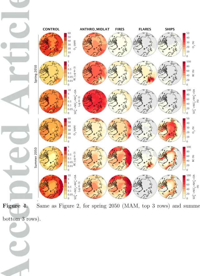
Results for spring 2050 are shown in Figures 4 and 5. Even though Arctic shipping emissions of BC increase by 55 % between spring 2012 and 2050, they remain too low to have a strong impact on surface BC concentrations or BC deposition. Between 2012 and 2050, the contribution from remote anthropogenic emissions to surface BC and BC deposition decreases from 60 % to 50 % approximately, because of the decrease in global anthropogenic BC emissions in the ECLIPSEv5 CLE scenario (−27 % in domain d1). The contribution from biomass burning emissions, assuming constant 2012 emissions, remains low during spring. Flares also remain an important springtime source of BC and BC deposition, especially in northwestern Russia. The relative contribution of flaring to Arctic BC increases slightly compared to 2012 (from 10 % to 15 % in the central Arctic) because of the small projected increase in flaring BC emissions and the strong decline in global BC emissions.

In summer 2050, Figure 4 shows that local shipping emissions become the main source of Arctic surface ozone (up to 35 %, 10 ppbv) and surface aerosol pollution (up to 70 %,

250 ng m−3 for BC; 50 %, 1 µg m−3 for other aerosols) along diversion shipping lanes

in use in July and August. Increases in sulfate, nitrate, and ammonium aerosols from

Arctic shipping are again likely due to a combination of higher emissions (NO_x, SO₂),

in-creased oxidant levels (OH), and changes to aerosol chemistry (as discussed in Section 3.1. However, an important caveat is that this does not include the effect of changing

mete-orology and sea ice in 2050, since they are kept constant between 2012 and 2050 in our simulations. These climate-related changes could have an important effect on the ozone chemistry during sumer in the Arctic, by e.g. increasing dry deposition (due to decreased atmospheric stability and larger open ocean surfaces) and decreasing photolysis [due to the decreased albedo from reduced snow and sea ice cover; Voulgarakis et al., 2009].

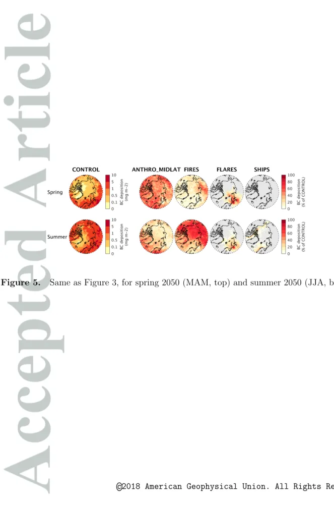
Shipping emissions are responsible for most of the total surface BC along Arctic shipping lanes in summer 2050, but do not cause a strong increase in BC deposition fluxes at the surface (Figure 5). In our simulations, BC deposition is mainly due to wet removal, which also depends on BC concentrations aloft that are insensitive to surface Arctic shipping emissions (Section 4). The contribution of shipping emissions to total BC deposition is higher along the Northwest Passage than over the Northern Sea Route, because of lower background deposition along the Northwest Passage. However, in agreement with Browse

et al. [2013] and M´en´egoz et al. [2013], we find that diversion shipping, even in this “High

Growth” future scenario, does not strongly increase BC deposition over snow and ice (at most 4 to 8 % locally during summer; the snow and ice limit is shown in Figure 1). This is due to the short residence time of Arctic shipping BC (1.4 days during summer 2050), limiting transport away from the shipping lanes and onto ice or snow. Deposition of shipping BC over sea ice could be even lower using realistic weather conditions and sea-ice for 2050, due to the lower sea-sea-ice available for BC to deposit on [Wang and Overland , 2012] and to the reduced aerosol lifetime from increased precipitation [Jiao and Flanner , 2016]. In our simulations, BC lifetime in the Arctic is mostly controlled by wet removal (96 % of the total BC deposition in the Arctic). Although there is to our knowledge no direct observational constraint on the short BC lifetime found in the Arctic summertime marine

boundary layer, we note that, using a similar setup, WRF-Chem was able to reproduce the observed summertime BC concentrations near the Arctic Ocean [Marelle et al., 2017] at Zeppelin (Svalbard), Nord (Greenland) Alert (Canada), and Barrow/Utqia ˙gvik (Alaska), giving some confindence in these results.

4. Future (2050) local and remote emission contributions to vertical

distributions Arctic aerosols and ozone

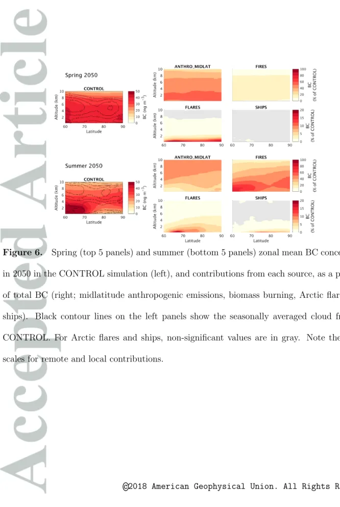
The radiative effects of aerosols and ozone do not scale with surface concentrations, and are more strongly related to total column burdens. Radiative effects are also known to be very sensitive to vertical pollutant distributions [Lacis et al., 1990; Rap et al., 2015; Flanner , 2013]. In addition, wet deposition of BC is sensitive to aerosol concentrations at higher altitudes, in or below clouds. For these reasons, and to better understand the origin of Arctic aerosols and ozone, Figures 6 and 7 show the seasonally averaged zonal mean BC and ozone contributions from different emission sources in 2050 (results in 2012 are qualitatively similar, except that shipping has much smaller impacts). These figures also show the average cloud cover in the CONTROL simulation, indicating that clouds are often present (mean cloud cover up to 25 %) at the surface and at altitudes from 4 to 8 km in the Arctic.

Figure 6 indicates that mid-latitude anthropogenic and biomass burning emissions are responsible for the majority of the Arctic-wide burden of aerosol pollution. Remote an-thropogenic sources have a strong influence on BC throughout the troposphere during spring, and are also a strong source of BC during summer, especially between 3 to 9 km

and at the surface north of 75° N. Biomass burning has a relatively small influence on BC

during summer, especially south of 75° N, close to boreal fire sources. These results are in agreement with those from Xu et al. [2017] for spring. During summer, Ikeda et al. [2017] and Stohl et al. [2013] found even higher biomass burning contributions to BC.

In Figure 6, at higher altitudes, the sum of the individual quantified BC contributions (ANTHRO MIDLAT+FIRES+FLARES+SHIPS) adds up to less than 100 % of CON-TROL BC. In this study, we only quantify the contributions of the following sources of

Arctic aerosols and ozone: anthropogenic emissions south of 60° N, biomass burning

emis-sions, shipping emissions north of 60° N and flaring emissions north of 60° N. All of the

other sources (e.g., the stratospheric source, sources outside of the domain boundary, Arc-tic emissions from the residential or road transport sectors) are included in CONTROL and in all of the sensitivity simulations, but their individual contributions to Arctic BC are not quantified, since no simulations are performed with these sources turned off. It is clear in Figure 6 that some of these unquantified contributions have an important in-fluence on high-altitude BC in the Arctic in spring. Since BC transport to the Arctic is quasi-isentropic, these unquantified contributions to high-altitude Arctic BC are likely to originate from the lower latitudes, e.g. from the tropics or even the southern hemisphere (Figure 4.3 of AMAP [2015]), south of the d1 domain boundary conditions specified by the MOZART4 model. Indeed, AMAP [2015] showed that even emissions in the southern hemisphere could be responsible for approximately 10 % of Arctic BC burdens. At the surface, the sum of individual BC contributions is also less than 100 % during spring. This is because we focus in this study on remote emissions and on the ermerging Arctic gas flaring and shipping emissions, but do not quantify the contribution from other local Arctic BC sources, such as domestic combustion, which has been shown to be a relatively

strong source of surface Arctic BC in winter and spring [Stohl et al., 2013]. However, these points do not affect the conclusions of this study, since the contribution of one source of interest (e.g. Arctic Flares) to Arctic BC can be estimated without estimating the contribution from all the other potential sources.

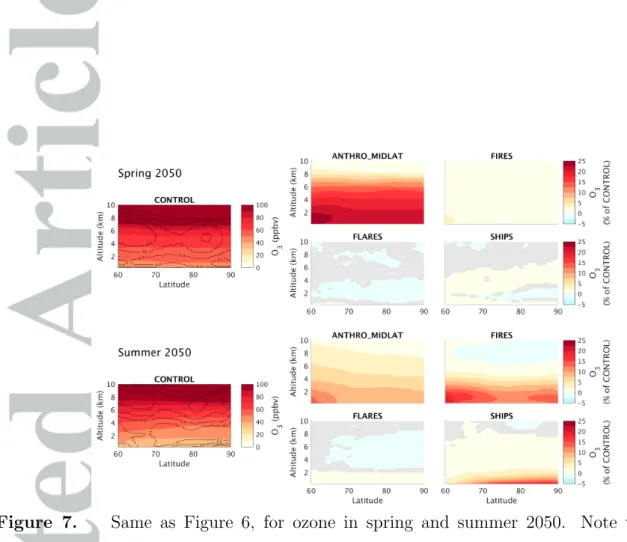
With regard to ozone, Figure 7 shows that non-methane remote anthropogenic emis-sions make an important contribution to ozone in the lower Arctic troposphere during spring, while biomass burning emissions have a very limited role, in agreement with We-spes et al. [2012]. Anthropogenic emissions make a small relative contribution in the upper troposphere during spring, due to the large stratospheric source [not quantified here, see e.g. Wespes et al., 2012]. However, absolute enhancements due to remote an-thropogenic emissions are significant, 5 to 13 ppbv at altitudes 5 to 8 km. During summer, biomass burning emissions contribute more than remote anthropogenic emissions to lower tropospheric ozone. This contrasts to results from Wespes et al. [2012], who found that Northern American and European anthropogenic emissions were the dominant sources of summertime Arctic ozone at low altitudes. As already noted, Wespes et al. [2012] focused on a limited time period during summer 2008, using a different model, and significant dis-agreement remains between models regarding boreal fire impacts on Arctic ozone Arnold et al. [2015].

Arctic flaring emissions have an important effect on the BC zonal mean, 5 to 20 %, comparable to results from Stohl et al. [2013]. This effect is mostly confined below 2 km. As discussed in Section 3, flaring has a more localized influence during summer, due to stronger total deposition and to the northern shift of the Arctic Front. Arctic flares have a negligible effect on ozone levels.

In 2050, Arctic shipping makes a relatively small contribution to zonal mean BC con-centrations, even at the surface during summer (at most, 10 % below a few hundred

meters at latitudes 70° N to 80° N). However, future Arctic shipping has a larger effect on

summertime ozone in the lower troposphere (5 to 20 % below 2 km), especially at higher latitudes.

5. Present-day and future Arctic radiative effects due to local and remote emissions.

In order to compare the contribution of each source to the local radiative budget, we

calculate with the WRF-Chem model the Arctic-wide average (60° N to 90° N) of the

radiative effects at the top-of-atmosphere (TOA) of aerosols and ozone from local and remote sources of Arctic pollution.

5.1. Calculating the radiative effects of short-lived pollutants in WRF-Chem The RRTMG module in the WRF-Chem model calculates radiative fluxes at TOA, taking into account predicted aerosols. In this work, RRTMG was also modified to use model-predicted ozone for radiative calculations, instead of climatological values. In these simulations, the RRTMG module is called 3 times at every radiative time step, first with all species taken into account, then without aerosols, and without ozone, in order to calculate the total direct radiative effects at TOA of aerosols and ozone. The direct effect from a specific source (e.g. Arctic shipping) is calculated as the difference in total direct effect between the simulations with (CONTROL) and without (e.g. NOSHIPS) for this source. The direct effect of aerosols includes the effect of changes in BC, sulfate, nitrate, ammonium and OA concentrations due to a particular source, but the effect of these different components is not estimated separately here. The calculation of direct effects

does not take into account the effect of rapid adjustments in stratospheric temperatures, tropospheric temperatures and water vapor; i.e., calculated direct effects presented here are the so-called ”instantaneous radiative forcings” [e.g., Myhre et al., 2013a].

WRF-Chem also calculates aerosol activation in liquid clouds and the resulting ef-fects on cloud properties, including cloud albedo and cloud lifetime, for both grid-scale clouds [Morrison microphysics scheme; Morrison et al., 2009] and sub-grid clouds [KF-CuP scheme; Berg et al., 2015]. As a result, changes in aerosol concentrations, com-position and size between two simulations, e.g., CONTROL and NOSHIPS, may also change cloud properties [aerosol first and second indirect effects; Twomey, 1977; Albrecht , 1989]. Semi-direct aerosol effects [Hansen et al., 1997] are also taken into account, since predicted aerosol optical properties (and ozone concentrations) are coupled to radiation calculations within WRF-Chem, and have an influence on heating rates, temperature and relative humidity profiles, causing additional changes in cloud formation, cloud properties, and cloud lifetime. As a result, we calculate the direct+indirect+semi-direct radiative ef-fects at TOA from a specific source as the difference of total upwelling radiative flux at TOA between the simulations with and without a particular source. Since the direct effect of aerosols and ozone is also known separately from the calculations presented above, we can extract from these runs the indirect+semi-direct effects for each source. The radiative effect of snow albedo changes due to BC deposition is not included in our calculations, nor the effect of ozone produced from methane and related long-term feedbacks, although they can be substantial and account for approximately half of the direct effects of BC and ozone respectively [AMAP , 2015].

For Arctic shipping and flaring, the calculations are performed for each ensemble mem-ber, and a Student t-test is then performed to assess whether each radiative effect (e.g. direct aerosol effect of shipping) is significant at the 95 % level, following the approach presented in Section 2.3. Only statistically significant values are given and discussed in the following.

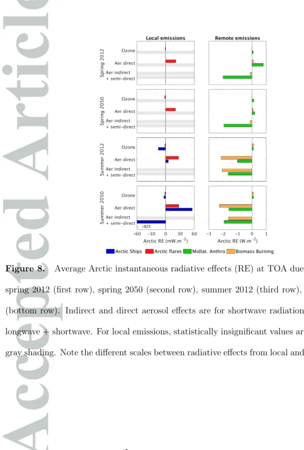
5.2. Direct and indirect radiative effects of aerosols and ozone in the Arctic

Figure 8 shows the calculated radiative effects at TOA in the Arctic (latitude > 60° N)

of aerosols and ozone due to present-day and future emissions from Arctic shipping and flaring, as well as biomass burning and mid-latitude anthropogenic emissions. Positive radiative effects at TOA have a global warming effect, while negative values have a global cooling effect.

5.2.1. Current and future radiative effects from remote anthropogenic sources and from biomass burning

Radiative effects due to biomass burning and mid-latitude anthropogenic emissions are approximately two orders of magnitude larger than those from local Arctic shipping and flaring emissions. The only exception is the indirect effect of shipping emissions in summer 2050 (see discussion below). The larger role of remote sources is a consequence of the larger emission amounts, leading to higher pollution burdens in the Arctic, as discussed in previous sections.

Present-day biomass burning and remote anthropogenic aerosols have a combined direct

effect in the Arctic of 0.9 W m−2 during spring, and −3.1 W m−2 during summer. These

combined effects are more intense than estimated by the AEROCOM phase II models [the

2017]. In our simulations, the direct aerosol radiative effect is net positive in the Arctic in

spring (0.9 W m−2), as for half of the AEROCOM phase II models [Sand et al., 2017], due

to the high albedo of snow and ice. It is well known that even aerosols with low single-scattering albedos (i.e. containing little black carbon) can have a positive direct effect over highly reflective surfaces [Pueschel and Kinne, 1995]. In summer, we estimate a strong

negative direct aerosol effect (−3.1 W m−2, see Figure 8), lower by −2.7 W m−2 than Sand

et al. [2017]. This difference could be due, in part, to the fact that several AEROCOM phase II models do not represent SOA and ammonium aerosols, which could enhance the global direct aerosol effect by 30 % [Myhre et al., 2013b]. In addition, AEROCOM phase II models calculate the direct aerosol effect as a difference between present-day (2000) and preindustrial (1850) emissions, when our simulations use the difference between present-day (2012) emissions and zero emissions. This last point could be especially important for the DRE of biomass burning aerosols, since preindustrial biomass burning emissions are far from zero due to the contribution of natural wild fires in preindustrial times. In order to compare our results to Sand et al. [2017], we also calculated the average JJA 2012 aerosol optical depth at 550 nm (AOD) in WRF-Chem, interpolated at 9 Arctic observing stations (Alert, Canada; Ny lesund, Svalbard; Barrow, Alaska; Kangerlussuaq, Greenland; Resolute Bay, Canada; Bonanza Creek, Canada; Yakutsk, Russia; Andenes, Norway; Tiksi, Russia). We found that the mean AOD in WRF-Chem at these sites is 0.17, substantially higher than in Sand et al. [2017] where the multimodel mean is 0.078 (individual models from 0.028 to 0.15). This difference in AOD could be due to stronger aerosol transport to the Arctic in summer 2012, or to intermodal differences (e.g. a longer aerosol lifetime in the Arctic free troposphere in WRF-Chem). However, this difference

in AOD is unlikely to be due to differences in emissions since summertime anthropogenic and biomass burning emissions from AEROCOM phase II [Lamarque et al., 2010] for BC,

SO₂, and Organic Carbon in domain d1 are 20 %, 17 %, and 19 % higher than in the

present study, while only NO_x emissions are lower, by 8 %.

The sum of aerosol indirect and semi-direct effects due to present-day anthropogenic

and biomass burning emissions in spring (−2.1 W m−2) and summer (−3.7 W m−2) are

of the same magnitude but stronger than estimates for the indirect effect of aerosols in

the high Arctic (68° N to 90° N) for 2003 by Shindell [2007], −0.25 W m−2 in spring;

−1.75 W m−2 _{during summer.}

The total (SW+LW) radiative effect of ozone from midlatitude anthropogenic emissions

is ∼ 0.1 W m−2 in spring and summer. The effect of ozone from biomass burning emissions

during summer is also ∼ 0.1 W m−2. These values are similar to the annual average

radiative effect of ozone in the Arctic of 0.15 W m−2 estimated by Collins et al. [2013].

Note that these values do not include the effect of methane emissions, which are estimated to be responsible for nearly half of the historical radiative forcing of ozone [Stevenson et al., 2013].

Between 2012 and 2050, global anthropogenic emissions of BC decrease in the

ECLIP-SEv5 CLE scenario, while SO₂ and NO_x emissions increase. As a result, the direct effect

of aerosols from remote anthropogenic sources is more negative in 2050 compared to 2012,

changing by ∼ −0.6 W m−2 in both spring and summer. Such a change would reverse

esti-mated recent trends in the Arctic direct aerosol effect, since Breider et al. [2017] calculated

changes of ∼ +0.48 W m−2 between 1980 and 2010 due to declining Arctic aerosol loads

the ECLIPSEv5 CLE scenario, some scenarios project strong reductions in future sulfur dioxide emissions, reducing the sulfate load globally and in the Arctic [e.g. Representative Concentration Pathways scenarios, Lamarque et al., 2011]. Such reductions would cause a positive change in direct radiative effect relative to present-day [Gillett and Von Salzen, 2013].

Biomass burning emissions are kept constant in our experiments, and as a result the associated direct radiative effects also remain approximately constant, with some small differences in 2050 likely due to model non linearities. However, since these non linearities are higher for the cloud response, indirect effects from biomass burning are noticeably different in summer 2050 and in summer 2012 despite constant emissions.

5.2.2. Current and future radiative effects from local Arctic flaring and ship-ping

Arctic flaring emissions have small but significant positive direct radiative effects (20 to

30 mW m−2) in spring and summer 2012 and 2050 (Figure 8), which are comparable to

earlier annual estimates from AMAP [2015]. This is due to their large influence on Arctic BC. However, we find no significant indirect and semi-direct aerosol effects from Arctic flares, and very weak radiative effects for ozone. Arctic flaring emissions are relatively stable between 2012 and 2050 in the CLE scenario, and as a consequence radiative effects from Arctic flares do not change much between present and future in our simulations.

Present-day Arctic shipping aerosols have a small positive direct effect during summer

(∼ 6 mW m−2 in 2012, ∼ 55 mW m−2 in 2050), whereas earlier studies found a negative

direct effect [e.g., Ødemark et al., 2012]. This positive net direct effect from shipping aerosols seems to be driven by the effect of BC over sea ice, even though shipping aerosols

are mostly found over the open ocean and only occasionally over snow and ice. Sand et al. [2017] showed that, during summer, anthropogenic and biomass burning aerosols in the Arctic have a strong positive direct effect over sea ice and a very weak negative effect over open water. In 2050, the positive direct effect of shipping aerosols increases due to higher emissions, but remains low compared to the effects of remote sources. This is a consequence of the relatively small contribution of Arctic shipping emissions to the total aerosol burden in the Arctic. In addition, aerosols from ships are mostly located below and within clouds (Figure 6), which can reduce their direct effect but increase their indirect and semi-direct effects.

Present-day indirect effects from Arctic shipping emissions (spring and summer) are not found statistically significant by our method (p value = 0.15 during summer). Previous studies [Ødemark et al., 2012; Marelle et al., 2016] have reported large negative indirect effects from Arctic shipping emissions during summer, but we find here that internal variability in a coupled model such as WRF-Chem is large enough to mask this relatively strong signal. These results suggest that larger ensembles or longer integration periods are needed to quantify moderate indirect effects in models. In contrast, we estimate a large negative indirect and semi-direct aerosol radiative effect from Arctic shipping of

−0.8 W m−2 _{in summer 2050, This is due to increased diversion shipping in the scenario}

employed here. This value is similar in magnitude to the indirect effects of aerosols from remote anthropogenic and biomass burning emissions. This large future effect is likely due to the indirect effects of increased concentrations of hydrophillic sulfate, ammonium and nitrate aerosols, which are significantly higher in 2050 due to summertime diversion

globally by the use of shorter diversion shipping routes through the Arctic, reducing global warming in the long-term [Fuglestvedt et al., 2014]. In addition, Dalsøren et al. [2013] showed that moderate diversion shipping in 2030 combined with strong emission reduction measures could lead to a decrease in the Arctic sulfate burden, causing warming compared to the present day. This is not the case in our study due to the extreme growth in traffic in the ”High Growth” diversion scenario for 2050. These results indicate that predictions of future shipping impacts on climate are very sensitive to assumptions used to estimate future emission scenarios.

Surprisingly, we find that ozone from Arctic shipping has a small negative effect at

TOA (∼ −15 mW m−2 in summer 2012, ∼ −4 mW m−2 in summer 2050), even though,

as a greenhouse gas, the radiative effect of ozone is usually positive at TOA. To our knowledge, this is in contrast with all previous estimates of the radiative effect of ozone from Arctic ships, e.g. Ødemark et al. [2012], Dalsøren et al. [2013], Fuglestvedt et al. [2014]. This negative effect is due to the LW effect of ozone and to temperature inversions in the Arctic. Figure 7 shows that ozone pollution from Arctic shipping is confined close to the surface. In the model, air temperatures in these lower layers are often warmer than surface temperatures, a situation known as a temperature inversion, which is commonly observed in the Arctic [e.g., Devasthale et al., 2010]. As a result, enhanced ozone in these warmer atmospheric layers increases LW emission and heat loss to space. In the CONTROL simulation, temperature inversion frequencies in the Arctic are 70 % during spring, 58 % during summer. Using clear-sky satellite measurements, Devasthale et al. [2010] estimated similarly high inversion frequencies of 88 to 92 % during winter, and 69 to 86 % during summer. Rap et al. [2015] also showed that increasing ozone at the surface

in the Arctic and Antarctic could cause a negative LW effect [Figure 1b in Rap et al., 2015], although they estimated that this effect would be compensated by an associated positive SW effect. This compensation does not occur in our simulations, either because the SW effect is lower due to ozone enhancements being often located below clouds, or because the LW effect is larger than in Rap et al. [2015] due to stronger or more frequent temperature inversions. Overall, this negative net effect from ozone can be expected to depend strongly on the vertical ozone profile from a given source, and on the strength, pattern, and frequency of temperature inversions in the model. Since Arctic shipping

O₃ increases LW emission from the warm near-surface layers, it will also increase LW

backradiation to the surface. As a result, the LW effect associated with shipping O₃

could warm the surface but cool the lower troposphere, and the combination of these two competing effects may have only limited effects on Arctic surface temperature, although it could decrease atmospheric stability. Flanner et al. [2018] have recently studied the effect of greenhouse gas enhancements in inversion layers on surface temperature, and found that the likely resulting effect would still be a warming of the Arctic surface.

In 2050, the negative LW effect from shipping O₃ is larger than in 2012 (Figure S1a

and S1b in the electronic supplement), because of the higher O₃ shipping enhancements

from larger emissions. However, in 2050 the positive SW effect is increasing more than the LW effect, especially over sea ice (Figure S1c and S1d in the electronic supplement), and the resulting future total effect (SW+LW, shown in Figure 8) is thus reduced. We attribute this large increase in the SW effect to the high diversion shipping emissions in

the central Arctic ocean, which increase O₃ over the ice pack, where the SW O₃ effect

with O₃. Compared to these simulations using constant meteorology and sea-ice, it is

likely that there would be less O₃ over sea ice in 2050 along with reduced sea ice, since

diversion routes would only be operating far away from the ice edge, although ozone has a lifetime of several days and can also be transported far from where ship emission occurs. At the same time, there would also be less inversions in 2050 since sea ice cover is a good proxy for temperature inversions in the Arctic [Pavelsky et al., 2011].

6. Conclusions

Local Arctic emissions from shipping and resource extraction are currently growing and could become an important source of pollution in the Arctic, relative to anthropogenic and biomass burning sources emitted largely outside the Arctic. This study investigates the impacts of remote emissions (midlatitude anthropogenic, biomass burning) and emerging local emissions (Arctic shipping, Arctic gas flaring) on the distributions and radiative effects of aerosols and ozone in the Arctic. In this study, we have considered the effect of changing future emissions, but not the effect of the changing Arctic climate, including changing sea ice, which could also influence future Arctic aerosols and ozone and their impacts. Voulgarakis et al. [2009] showed that, in an ice-free Arctic, ozone would increase significantly during spring due to reduced bromine chemistry, and decrease significantly during summer due to reduced photolysis. Concerning aerosols, Jiao and Flanner [2016] have showed that warming-induced transport changes and wet removal increases could decrease Arctic BC burdens by 14 %, further reducing the contribution of long-range transport to Arctic aerosols and ozone.

with-concentrations (surface, troposphere), BC deposition fluxes, and radiative effects, in spring and summer for the present-day (2012) and the future (2050). Future projections use a scenario taking into account current planned emission reduction legislation (ECLIPSEv5

CLE), projecting lower 2050 BC and higher SO₂ and NO_x emissions relative to 2012

in the Northern Hemisphere, with slowly growing Arctic flaring emissions. We also use high-growth projections of future shipping emissions in the Arctic, including future diver-sion shipping through the Arctic Ocean. Our results assume constant biomass burning emissions compared to 2012. The key novel points in this study are the following:

First, this study quantifies the relative impacts of emerging local sources of Arctic pol-lution (Arctic shipping and Arctic gas flaring emissions), compared to remote sources of pollution. The importance of this issue has been highlighted in recent papers, [Arnold et al., 2016; Law et al., 2017], but this comparison has not to our knowledge been inves-tigated in previous studies. In line with previous work on Arctic pollution, we find that long-range transport of pollution from mid-latitude anthropogenic emissions and biomass burning emissions is the main source contributing to pollution burdens in the Arctic (for 2012 and 2050 emissions), with anthropogenic pollution dominating in spring and biomass burning during summer. However, we find that local sources already have an important influence on surface and lower tropospheric concentrations of ozone and aerosols (BC,

NO₃–, NH₄+, SO₄2 –). With 2012 emissions, Arctic shipping makes an important

contribu-tion to surface ozone (15 to 25 % of total surface ozone) in the Norwegian and Barents Sea region during summer. This is caused by a strong increase in summertime surface OH

concentrations (∼ by a factor of 2 in the Norwegian Sea) due to shipping NO_x emissions.

Arctic gas flaring is estimated to be a major source of current surface BC in spring and summer, and of BC deposited over snow and ice in spring over northern Russia and the Kara Sea. We show that these significant contributions could continue in the future, and that the relative influence of local flaring BC in the Arctic could increase due to pro-jected anthropogenic BC emission reductions in the mid-latitudes. In contrast to some previous studies, we do not find that gas flaring is a significant source of Arctic surface BC outside of northern Europe, northern Russia and the Kara Sea. Due to the projected growth in Arctic shipping emissions associated with diversion shipping in 2050, Arctic shipping could become a major source of surface ozone (up to +10 ppbv) and aerosols (locally, the main source of surface BC) during the Arctic summer. Diversion shipping does not contribute significantly to BC deposition over snow and ice due to efficient wet BC removal over the open Arctic Ocean at this time of year. The relative contribution of remote anthropogenic emissions could be further reduced by emission control in the midlatitudes: the ECLIPSEv5 CLE scenario used for future projections contains lower BC emissions in 2050 than in 2012. However, such predictions are very sensitive to the uncertain evolution of future global emissions.

Second, this study gives an estimation of the indirect aerosol effects from remote and local Arctic sources using a model resolving aerosol activation in clouds explicitly. Quanti-fying radiative effects due local Arctic emissions is complicated by model internal variabil-ity due to small perturbations in concentration distributions and aerosol-cloud feedbacks. Here, we use ensemble simulations to diagnose statistically significant direct and indirect radiative effects. Our results show that present-day biomass burning and remote

in spring and −3.7 W m−2 in summer. In comparison, we find a combined direct effect

of +0.9 W m−2 during spring, and −3.1 W m−2 during summer. Compared to these

remote sources, we estimate small present-day radiative effects from shipping and gas

flaring with 2012 emissions (at most ∼ 25 mW m−2 for the direct aerosol effect of Arctic

flaring, both in spring and summer). The indirect aerosol effect due to present-day local Arctic emissions could not be assessed using our method, since the values were found to be too small to be statistically significant. However, a major finding of this study is that the increased aerosol load due to future shipping could cause a very strong negative

indirect and semi-direct effect of −0.8 W m−2, which is comparable in magnitude to the

direct and indirect effects due to anthropogenic and biomass burning emissions. In our simulations, this large effect is due to the location of shipping aerosols, which are often present within clouds, particularly in the summer when Arctic diversion shipping occurs. The radiative impacts of BC deposition could not be investigated here due to the lack of a detailed snow-albedo model within our version of WRF-Chem. However, the results presented here could be used in future work to assess the radiative effects of remote and local sources due to these processes.

Third, in contrast to previous studies, we diagnose a small significant negative radiative

effect at TOA due to ozone from Arctic shipping (∼ −15 mW m−2 in summer 2012,

∼ −4 mW m−2 _{in summer 2050). This is due to the frequent temperature inversions in}

the Arctic, and to the fact that ozone produced from Arctic shipping is often located in atmospheric layers that are warmer than the surface.

Our results indicate that, even though emissions from local sources are relatively low compared to global totals, they already have significant impacts in the Arctic. Arctic

shipping emissions are one of the major sources of surface OH and ozone, and Arctic flares are a major source of surface BC concentrations and BC deposition. This influence can also be expected to increase in the future, especially if diversion shipping develops rapidly. In this case, Arctic shipping could become a major source of surface aerosol and ozone pollution in the summer, and could potentially have very large negative local radia-tive effects at TOA due to their indirect effects. However, even for worst-case future local emission scenarios, mid-latitude anthropogenic emissions and biomass burning emissions can be expected to remain the main sources of ozone and aerosol burdens in the Arctic troposphere, as well as the main sources contributing to aerosol and ozone radiative ef-fects in the Arctic. However, in order to improve our confidence in these results, improved quantification of aerosol-cloud feedbacks as well as processes influencing the vertical dis-tribution and loss of pollutants are needed, together with refined methodologies to assess pollutant radiative effects under a range of possible emission scenarios.

Acknowledgments. We acknowledge funding from the European Union (Framework 7 programme) ICE-ARC (Ice, Climate, Economics - Arctic Research on Change) project, under Grant Agreement 603887 and the French Chantier Arctique Pollution in the

Arctic System (PARCS) project. Computer resources were provided by IDRIS HPC

under GENCI, and by IPSL CICLAD/CLIMSERV. Louis Marelle acknowledges fund-ing from TOTAL SA through an ANRT CIFRE PhD grant. We thank colleagues at PNNL (Jerome D. Fast, Manish Shrivastava, Larry K. Berg, Richard C. Easter) and CICERO (Maria Sand) for helpful discussions. The WRF-Chem model is available at http://www2.mmm.ucar.edu/wrf/users. Meteorological and chemical data from NCEP and MOZART4, used for initial and boundary conditions, can be found at https://rda.

ucar.edu/ and https://www.acom.ucar.edu/wrf-chem/mozart.shtml. DMS oceanic data is available at https://www.bodc.ac.uk/solas_integration/implementation_

products/group1/dms/documents/dmsclimatology.zip. RCP8.5 shipping emissions,

ECLIPSEv5 anthropogenic emissions, Arctic shipping emissions for local and di-version shipping, and FINNv1.5 fire emissions are available at https://tntcat.

iiasa.ac.at/RcpDb/dsd?Action=htmlpage&page=download, http://www.iiasa.ac.

at/web/home/research/researchPrograms/air/ECLIPSEv5.html, http://envs.au.

dk/en/knowledge/air/emissions/projects/arctic-ship-emissions/, http://coast. cms.udel.edu/ArcticShipping/, http://bai.acom.ucar.edu/Data/fire/.

References

Albrecht, A., Bruce (1989), Aerosols, cloud microphysics, and fractional cloudiness, Sci-ence, 245 (4923), 1227–1230, doi:10.1126/science.245.4923.1227.

AMAP (2015), Amap assessment 2015: Black carbon and ozone as arctic climate forcers, Tech. rep., Arctic Monitoring and Assessment Programme (AMAP), Oslo, Norway. ˚

Angstr¨om, A. K. (1929), On the atmospheric transmission of sun radiation and on dust

in the air, Geogr. Ann., 11, 156–166, doi:10.2307/519399.

Arnold, S., K. Law, C. Brock, J. Thomas, S. Starkweather, K. von Salzen, A. Stohl,

S. Sharma, M. Lund, M. Flanner, T. Pet¨aj¨a, H. Tanimoto, J. Gamble, J. Dibb,

M. Melamed, N. Johnson, M. Fidel, V.-P. Tynkkynen, A. Baklanov, S. Eckhardt, S. Monks, J. Browse, and H. Bozem (2016), Arctic air pollution: Challenges and op-portunities for the next decade, Elementa, 4, 104, doi:http://doi.org/10.12952/journal. elementa.000104.