HAL Id: hal-03137748
https://hal.archives-ouvertes.fr/hal-03137748
Submitted on 11 Feb 2021
HAL is a multi-disciplinary open access
archive for the deposit and dissemination of
sci-entific research documents, whether they are
pub-lished or not. The documents may come from
teaching and research institutions in France or
abroad, or from public or private research centers.
L’archive ouverte pluridisciplinaire HAL, est
destinée au dépôt et à la diffusion de documents
scientifiques de niveau recherche, publiés ou non,
émanant des établissements d’enseignement et de
recherche français ou étrangers, des laboratoires
publics ou privés.
R. Sauzède, J. Johnson, H. Claustre, G. Camps-Valls, A. Ruescas
To cite this version:
R. Sauzède, J. Johnson, H. Claustre, G. Camps-Valls, A. Ruescas. ESTIMATION OF OCEANIC
PARTICULATE ORGANIC CARBON WITH MACHINE LEARNING. ISPRS Annals of
Photogram-metry, Remote Sensing and Spatial Information Sciences, 2020, V-2-2020, pp.949-956.
�10.5194/isprs-annals-V-2-2020-949-2020�. �hal-03137748�
ESTIMATION OF OCEANIC PARTICULATE ORGANIC CARBON WITH MACHINE
LEARNING
R. Sauz`ede1∗, J.Emmanuel Johnson2, H. Claustre1, G. Camps-Valls2, A.B Ruescas2
1CNRS-INSU, Sorbonne Universit´e, Institut de la Mer de Villefranche, Villefranche-Sur-Mer, France
2University of Valencia, Image Processing Laboratory, 46980 Paterna (Val`encia), Spain
KEY WORDS: Machine Learning, Parameter retrieval, Particulate organic carbon, Depth-resolved reconstruction,
Biogeochemical-Argo profiling floats, Global Ocean
ABSTRACT:
Understanding and quantifying ocean carbon sinks of the planet is of paramount relevance in the current scenario of global change. Particulate organic carbon (POC) is a key biogeochemical parameter that helps us characterize export processes of the ocean. Ocean
color observations enable the estimation of bio-optical proxies of POC (i.e. particulate backscattering coefficient, bbp) in the surface
layer of the ocean quasi-synoptically. In parallel, the Argo program distributes vertical profiles of the physical properties with a global coverage and a high spatio-temporal resolution. Merging satellite ocean color and Argo data using a neural network-based method has already shown strong potential to infer the vertical distribution of bio-optical properties at global scale with high space-time resolution. This method is trained and validated using a database of concurrent vertical profiles of temperature,
salinity, and bio-optical properties, i.e. bbp, collected by Biogeochemical-Argo (BGC-Argo) floats, matched up with satellite ocean
color products. The present study aims at improving this method by 1) using a larger dataset from BGC-Argo network since 2016 for training, 2) using additional inputs such as altimetry data, which provide significant information on mesoscale processes
impacting the vertical distribution of bbp, 3) improving the vertical resolution of estimation, and 4) examining the potential of
alternative machine learning-based techniques. As a first attempt with the new data, we used some feature-specific preprocessing routines followed by a Multi-Output Random Forest algorithm on two regions with different ocean dynamics: North Atlantic and
Subtropical Gyres. The statistics and the bbpprofiles obtained from the validation floats show promising results and suggest this
direction is worth investigating even further at global scale.
1. INTRODUCTION
The ocean plays a crucial role in the climate of our planet by regulating the amount of atmospheric carbon dioxide. The mag-nitude of carbon sequestration in the ocean is driven by two dif-ferent mechanisms: the so-called physical and biological car-bon pumps. The latter is governed by the global export of particulate organic carbon (POC) from surface waters to the deep ocean. However, despite their importance, the processes involved in the biological carbon pump are still poorly con-strained. This essentially results from the paucity of global observations at the appropriate spatial and temporal resolution, and in particular in situ POC measurements. Therefore, and in order to start developing an in depth understanding and quan-tification of export processes at the context of global change, the first prerequisite is to acquire and/or develop data sets with improved spatio-temporal coverage.
The particulate backscattering coefficient (bbp) is widely used
as a bio-optical proxy for POC (e.g.Cetinic et al.,2012). bbphas
the advantage that it can be continuously measured in situ from robotic platforms, like Biogeochemical-Argo (BGC-Argo)
pro-filing floats (Claustre et al.,2020;Roemmich et al.,2019) or
retrieved from satellite remote sensing. Thus, bbpis a key
bio-optical property for studying the space-time dynamics of the vertical distribution of POC, possibly opening a path for im-proving the characterization and quantitative assessment of the
biological carbon pump in the global open ocean (Boyd et al.,
2019;Briggs et al.,In Press). Satellite-derived products of POC
from bbp-based algorithms (Stramski et al., 2008) have also
∗Corresponding author
shown their potential to study the spatio-temporal distribution
of POC in the open ocean (Gardner et al.,2006;Loisel et al.,
2002;Stramska, 2009). However, such satellite-based estim-ates, restricted to the ocean surface layer, are insufficient in the context of global carbon cycle studies including carbon produc-tion and export.
A recent study showed that a neural network-based method could
efficiently extend surface bio-optical properties (i.e. bbp) to
depth by merging ocean color and hydrological data (SOCA method for Satellite Ocean-Color merged with Argo data to in-fer the vertical distribution of particulate backscattering
coeffi-cient;Sauz`ede et al.,2016). The interest in merging such type
of data resides in the fact that bbpand hence POC reflects the
stock of biological particles. This stock, derived from oceanic photosynthesis, is primarily driven by nutrient availability and light regime in the upper ocean which are both influenced by the physical forcing. Thanks to the Argo program operating and array of nearly 4000 robots measuring hydrological properties with much enhanced spatio-temporal resolution in the global
ocean (Roemmich et al.,2009) the resuting acquired data can
be combined with ocean color to retrieve the vertical
distribu-tion of bbpwith high resolution.
Data-driven techniques have become more popular within the
scientific community (Bergen et al.,2019) including the ocean
sciences (Malde et al.,2019). We are dealing with an
explo-sion of data from different sources of varying quality. Physical models are powerful but trial-and-error approaches to modi-fying these methods to accommodate new data streams is not possible. As an alternative, data-driven techniques within the machine learning (ML) community are numerous with many
approaches that can handle the large quantity, quality and
com-plexity (Reichstein et al.,2019;Camps-Valls et al.,2019). In
the context of the study mentioned above, a neural network-based method was trained using the BGC-Argo floats database
(∼4700 concurrent in situ temperature, salinity and bbp
pro-files). This method retrieves the bbpin the water column with
an error of ∼20% at a global scale.
Merging data from different sources presents many challenges and so the original authors with the SOCA method (SOCA2016
hereafter,Sauz`ede et al.,2016) used artificial neural networks
to find a function that predicts bbpvertically at a global scale.
The original methods used were able to predict bbpfor 10
differ-ent layers (from the surface to the depth where there is no more phytoplankton biomass). Although the database used in 2016 was representative of most open ocean oceanographic condi-tions in the global ocean, some areas were significantly under-sampled (e.g. southern ocean). It is therefore expected that using the new BGC-Argo database available today (with ∼ 5 times more data and a much better spatial coverage), the method could be greatly improved. In addition, it is timely to consider and evaluate a more powerful method that would allow to
estim-ate bbpat higher resolution along the vertical dimension which
is of great interest for carbon export applications.
The success of SOCA2016 motivated the effort to create depth-resolved global proxy of POC with higher space-time resolu-tion, a prerequisite for improving the characterization and quan-tification of export carbon fluxes. In particular, investigators of biogeochemical models have shown great interest and their need for such products, essential for the initialisation and valid-ation of biogeochemical models. Thus, this study takes place in the context of the European Copernicus Marine Environ-ment Monitoring Service (CMEMS), one challenges of which is to improve SOCA2016 to have high level 3D gridded global products of POC (with associated estimation errors), to support biogeochemical model data requirements for their improvements. The current study is aimed to improve upon the SOCA2016 method (upgraded method hereafter referred as SOCA2020) by 1) using the large amount of new acquired data from BGC-Argo floats network since 2016, 2) using additional inputs such as the sea level anomaly which could give significant informa-tion about sub-mesoscale processes the vertical distribuinforma-tion of phytoplankton biomass and hence of POC, 3) replacing some inputs such as the ocean color chlorophyll a concentration and
bbp by satellite reflectances to avoid additional errors due to
ocean color algorithms, 4) improving the vertical resolution
of the outputs (bbpretrieval) and 5) investigating the potential
of alternative machine learning-based techniques that could be more efficient and additionally could estimate the retrieval er-ror associated to the outputs, an essential point in the context of modelling.
2. DATA AND METHODS
The BGC-Argo database used in this study is composed of con-current vertical profiles of temperature, salinity and particulate
backscaterring coefficient (bbp) merged with satellite products.
First, we present more in details BGC-Argo measurements. Then, the procedure for the matchup between BGC-Argo and satellite observations is given in detail. The third section presents the machine learning models envisaged to carry out this study.
2.1 BGC-Argo measurements
Profiling floats typically collect measurements from 1000 m to the surface with a 1 m vertical resolution every 10 days. When the float surfaces, data is transmitted in real-time using Iridium communication. Physical Argo profiling floats are equipped with the standard conductivity-temperature-depth sensors that allow one to continuously measure the temperature and salinity
in the global open ocean since the early 2000s (Roemmich et
al.,2009). The integration of new biogeochemical sensors on
Argo floats has led to a new generation of floats, the BGC-Argo floats. These floats measure proxies of major biogeochemical
variables such as bbpthat is used to train and validate the SOCA
methods.
The BGC-Argo profiling floats used in this study are equipped with backscattering sensors that measure the angular scattering
coefficient at 124◦relative to the direction of light propagation
at wavelength of 700 nm. This measurement is transformed
into bbp(700) (hereafter bbp) followingSchmechtig et al.(2016).
The same quality control procedure as inSauz`ede et al.(2016)
was applied to each profile. Because of their log-distribution,
bbpvalues were log transformed.
2.2 BGC-Argo and satellite matchup database
For the development of the SOCA2020 method, the new in-puts are: 1) ocean color data: the reflectances (ρ) at 5 wave-lengths (412, 443, 490, 555 and 670 nm) and the Photosyn-thetically Available Radiation (PAR) and 2) altimetric data: the Sea Level Anomaly (SLA). The ρ are used in this study to
re-place Chl and bbpsatellite estimations used in SOCA2016, in
order to avoid additional input variability due to ocean color al-gorithms errors. For the long-term vision, PAR and ρ data come
from GlobColour satellite multi-mission data (Garnesson et al.,
2019) that were downloaded from the Copernicus Marine
En-vironment Monitoring Service (CMEMS, http://marine.coper-nicus.eu/). The matchup was done using the value of the closest pixel available with a 5-day window (before and after the obser-vation) and within a 5x5 pixel grid. This matchup procedure led to discarding ∼ 50% of the BGC-Argo profiles. The altimetric information (the SLA) is additionally used in SOCA2020 al-gorithm because it is highly linked to mesoscale structures that are known greatly influence the nitracline depth and so the ver-tical distribution of phytoplankton biomass and primary
pro-ductivity (L´evy et al., 2018). The altimetric data are issued
from the Global Ocean Multimission altimeter satellite gridded sea surface heights (available from CMEMS, daily data with a
0.25◦spatial resolution). The SLA is computed with respect to
a 20-year mean of sea surface height.
The resulting BGC-Argo and satellite matchup database ap-pears to be representative of a broad variety of hydrological and biogeochemical conditions prevailing in the global open ocean making the method applicable everywhere. Here, we focus our study on the North Atlantic Ocean (NA) and the oligotrophic
Subtropical Gyres (STG) (blue and red points in Figure1,
re-spectively). These two areas show quite different physical char-acteristics and dynamics: the NA ocean presents less salinity and lower temperatures than the STG throughout the year, and it presents strong mixing of water during winter (mixed layer depth, MLD, acquired by the BGC-Argo floats vary between 15 and 900 m). STG areas have a marked water stratification spe-cially during summer, with high sea surface temperature and deeper nitracline depth. These datasets are also representat-ive of most trophic conditions observed in the open ocean (i.e.,
Figure 1. Geographic distribution of the BGC-Argo profiles used to train and validate the model for the North Atlantic ocean
(blue) and the oligotrophic Subtropical Gyres (red).
from oligotrophic to eutrophic waters) and variations in phyto-plankton species composition and sizes.
2.3 Preprocessing
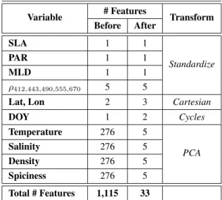
We implemented some basic preprocessing techniques to make the algorithms easier to train. Ultimately, there were over 1,100
features (Table1) with majority of the features coming from the
variables temperature, salinity, density and spiciness (that re-flects isopycnal water-mass contrasts). In addition, there were only 2,860 samples for the North Atlantic dataset and 1,353 samples for the Subtropical Gyres dataset. This is a bad samples-to-features ratio so we reduced the amount of correlation between the large number of features and alleviate this burden from the machine learning algorithms by implementing a series of simple transformations to better capture the most important aspects of our data.
The distributions for the core variables (SLA, PAR, MLD and the ρ at 5 wavelengths) were skewed and heavy tailed so we
did a simple standardization by removing the mean µx from
each feature and dividing by the standard deviation σx. There
was still very little correlation across variables except between
some of ρ variables like ρ412and ρ443. Some variables are
cyc-lic in nature so we converted the day of the year (DOY) variable to the corresponding sin and cos representation to better cap-ture the time component. The geographic coordinate system (lat, lon), while relevant in Earth sciences, can be very diffi-cult for machine learning algorithms due to the Earth curvature. For example, utilizing distance calculations like the euclidean distance between samples is non-trivial task in a geographical coordinate system compared to a Cartesian coordinate system. The trade-off is that the eventual predictions might produce er-rors due to the between-coordinate transformation erer-rors. So we converted the latitude and longitude (lat,lon) features into Cartesian (x,y,z) features to better accommodate euclidean-centric distance calculations.
The high dimensional variables (temperature, salinity, density and spiciness) were the ones with the largest amount of fea-tures. Each variable had one measurement per layer (all 276). So one option would have been to use the 1-to-1 layer corres-pondence between the input and the output. This would mean that each output for the y would have training data specifically from its corresponding layer which might proven to be effect-ive. However, we wanted to see if we could learn the relation-ships between the variables and not just the individual levels. Hence, we decided to use a Principal Components Analysis (PCA) decomposition on these variables. 5 PCA components
Variable # Features Transform
Before After SLA 1 1 Standardize PAR 1 1 MLD 1 1 ρ412,443,490,555,670 5 5
Lat, Lon 2 3 Cartesian
DOY 1 2 Cycles Temperature 276 5 PCA Salinity 276 5 Density 276 5 Spiciness 276 5 Total # Features 1,115 33
Table 1. The number of features before and after their respective transformations for different input variables used for the
machine learning models.
a) North Atlantic b) Subtropical Gyres
Cumulati v e Explained V ariance
Figure 2. The cumulative explained variance for the PCA components of the training data for the a) North Atlantic and b)
Subtropical Gyres.
were extracted from each variable thus reducing the number of features for the high dimensional variables from 1,104 (4×276) features to just 20 (4 × 5) features; significantly less. As shown
in Figure2, the cumulative explained variance for 5 PCA
com-ponents was ≥ 98% and ≥ 97% for the North Atlantic and for the Subtropical Gyres dataset, respectively. An argument can be made that extra 2-3% explained variance hidden in some of the remaining PCA components could have a big impact for
de-tecting rarer events and/or extreme bbpprofiles (i.e. the tails
of the output distribution). However, that would increase the number of redundant features of our input dataset which would make the machine learning algorithm harder to train.
The number of outputs for the bbp is 276 which is very high;
very unusual for a machine learning setting. Each output cor-responds to a depth so most of the variability was near the shallower regions for both the North Atlantic and Subtropical
Gyres datasets as seen in Figure3. This was verified through
the mean and standard deviation of the outputs as it was heavily skewed towards first 100 depths. So a simple log transform-ation was used to increase the spread of the distribution to be more Gaussian-like. Regardless, we still have the problem of having a large number of outputs which is very difficult for a machine learning model to train with a modest number of data points. We considered doing a PCA transformation on the out-put depths to reduce the number of outout-puts, but instead we de-cided against it for the first pass as it adds a level of complexity.
a) North Atlantic b) Subtropical Gyres
Depth
(m)
Figure 3. The BGC-Argo measured bbpprofiles for the training
dataset. The figure shows the mean and variance of the bbp
values vs. the depth (m) for the a) North Atlantic and b) Subtropical Gyres.
2.4 Machine learning models
Multi-output regression methods are a challenge even in the ma-chine learning community and there is no clear consensus about the best way to handle this problem in regression settings. Gen-erally, there are two main approaches to this problem from a machine learning perspective: a single model for each output
or a single model for all of the outputs (Xu et al.,2019). The
ideal case is to have a single model to account for the correlated outputs and this makes intuitive sense because we know that the outputs are well correlated; for example the overall shape of the output (depths in our case) would be captured instead of look-ing at individual parts. In addition, this approach is especially powerful when you have missing data and would like to use
semi-supervised learning (Alvarez et al.´ ,2012). However, this
approach can be more expensive, more difficult to train, and ul-timately there are not very many machine learning models that are explicitly designed to handle multiple outputs. Some ex-amples of ML models that can handle multi-output data include composition of functions like Neural Networks, Bayesian meth-ods like Gaussian processes, and ensemble methmeth-ods like
Ran-dom Forests (Reichstein et al.,2019;Camps-Valls et al.,2019;
Ruescas et al.,2018) but depending on the construction, it may or may not be taking into account the correlated outputs. The other approach is to use one model per output. This approach is useful if you have access to all the samples per output layer and if you do not want to restrict the number of algorithms to use. So one can use very sophisticated and fast algorithms with the only additional modification is a parallel training procedure to use each model per output. For this study we chose to use a single model trained for all of the outputs even though we do not have many samples and we have a very high number of output dimensions. We also chose some of the simplest class of models like linear regression and random forests. Although we have plans to do a more extensive comparison between the approaches, this is outside the scope of this paper and hence-forth when we refer to multi-output methods, we are assuming a single model that can handle multiple outputs.
We considered some baseline and robust methods for this ex-periment. We looked at 2 classes of models: linear models and ensemble models. We chose these models because they are an excellent choice for a first pass on new datasets and they are more easily intepretable. These “weakly” parametric models are robust, generalizable and can fit a large number of different datasets. This allows us to avoid making too many non-testable assumptions on the pre-processing step. The next step is to start adding more physical and intuitive constraints and expect-ations, e.g. priors and uncertainty estimates. This is future work but will require a Bayesian perspective of things. The baseline linear model we used is a simple regularized linear regression
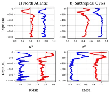
a) North Atlantic b) Subtropical Gyres
Depth (m) R2 R2 Depth (m) RMSE RMSE
Figure 4. Depth-associated statistics (R2top and RMSE bottom)
of the comparison of bbpvalues estimated from RF and RLR
models (in blue and red, respectively) to BGC-Argo measurements on the test dataset for the a) North Atlantic and b)
the Subtropical Gyres.
(RLR) model; the ridge regressor. We hypothesized that this model would perform well on the STG dataset but not as well on the NA dataset due to the non-linearities present in the shal-lower regions. The ensemble method used is a Random Forest (RF) regressor. This is an ensemble algorithm which averages several independent decision tree estimators. The variance is reduced because of the averages and in general, it is robust to overfitting. Furthermore, we can extract the feature importance from the model to see which features had the greatest impact on the predictions within our model. The models were trained using 1,000 estimators and a mean squared error (MSE)
cri-terion. Please see the github repositoryML4OCEANfor some
example notebooks highlighting the preprocessing routines and the machine learning models. For the experiment section, we will showcase the ridge linear regressor (RLR) and RF regressor results for the valdiation data. But we only show the RF model for the profiles as it was the better of the two models.
3. EXPERIMENTS
Two full machine learning pipelines were processed: one for the North Atlantic (NA) dataset and the other for the Subtrop-ical Gyres (STG) dataset. All preprocessing steps that did not involve normalization were done prior to splitting the data into training, testing and validation. Note that before this splitting, the time series from two BGC-Argo floats (one in NA region and the other in the STG regions, more precisely in the South Atlantic Subtropical Gyre, identified by their official World Met-eorological Organization number 6901486 and 3902121, re-spectively) were removed from the database to create an ”in-dependent data set” used for additional validation. After the split into training, testing and validation datasets, the normaliz-ation procedure was done on the training set only and then the transformation was done on the other two sets. Then we train the Multi-Output Random Forest on the training dataset. For the NA dataset, there were 2, 288 training samples, 572 testing samples and 352 validation samples. For the STG dataset, there were 1, 082 training samples, 271 testing samples and 26 valid-ation samples. With a 28-core on a SLURM server using
multi-processing, the training time took ∼30 seconds for NA dataset and ∼10 seconds for the STG dataset. Below, we showcase the results we obtained from this training procedure.
3.1 Test Data
Figure4shows the R2 and the RMSE for the North Atlantic
ocean (NA) and oligotrophic Subtropical Gyres (STG). In the NA, the RLR and the RF algorithms performs well in the layer very near to the surface and beyond 200 m depth. The ”middle” and upper layers (from ∼ 10 to 200 m) are where the weakest predictions are found. In contrast, RMSE values decrease with depth, with a maximum peak at ∼ 100 m. These weaker
predic-tions are related to the depths where bbpvalues show the more
variability (Figure3). Moreover, the minimum peak of
accur-acy at 400 m (low R2 and high RMSE in Figure4) is related
to a higher variance in the bbpvalues contained in the training
dataset at this specific depth. This variance is probably due to profile(s) with ”spikes” (POC intense increase at depth) that can be directly linked to POC export due to sinking particles. These ”extreme” profiles may have led to a decrease in the method performance for this specific layer. In the same way, the STG
dataset shows an increase of the R2 value first and then a
rel-atively unstable decrease with depth, until reaching a peak of lower accuracy and higher RMSE at around 200 m depth. This peak is more accentuated with the RLR model. This depth is
associated with the layer where bbpis more variable in STG
re-gions because of the so-called deep biomass maxima that can be found in these oligotrophic areas (between ∼ 150 - 200 m
depth,Mignot et al., 2014). RMSE values in the STG areas
show much more variability, related to the higher variance in the
input data shown in Figure3. However, the RMSE are lower for
STG in a quantitative way (range from 0.1 to 0.15 for STG area compared to a range from 0.15 to 0.4 for NA area) because of
the lower range of bbpvalues found in these oligotrophic gyres.
The highest R2 and lowest RMSE values very near the surface
for both areas with both models can be explained by the fact
that the methods should easily link surface bbp values to
sur-face satellite reflectance (ρ) inputs. Besides, some ocean color algorithms retrieving biogeochemical parameters from ρ at sev-eral wavelength are based on machine learning algorithms. To better understand the validation results and relate them to the input features and response of the model, the feature ranking for
the RF algorithm is shown in Figure5(for the entire output
do-main, not just a single layer). For the NA dataset, the most dom-inant features are the principal components of the density, tem-perature and salinity. Indeed, there is a lot of physical variab-ility in this area, that can explain the POC vertical distribution. For example, a strong winter mixing can bring phytoplankton biomass and POC up to 1000 m depth. In addition, the loca-tion seems to be also very important which was expected due to the variability in this area. We used NA data from high
lat-itudes to 0◦latitude (Figure1) so this area is representative of
very different trophic regimes (from high latitudes productive regions to the North Atlantic oligotrophic gyre). Surprisingly, less weight have the remote sensing reflectance, PAR and SLA variables, that are, those that affect more the upper layers. For the STG dataset, the location was the most important fol-lowed by some of the principal components for the temperature, salinity and density. The STG dataset is composed of 5 differ-ent gyres distributed on the planet whereas the NA dataset is much more spatially localized. Like the NA dataset, the reflect-ance and other variables like the MLD and PAR were not as im-portant. The MLD has less seasonal variability in this warmer
a) North Atlantic
b) Subtropical Gyres
Figure 5. The feature importance of the Random Forest algorithm for the test dataset for the a) North Atlantic and b) Subtropical Gyres. This plot explains the importance of each
feature as learned from the algorithm.
area where waters are almost always stratified. In these areas, the information from PAR input may be supported by the DOY (day of the year, sinus and cosinus transformed) inputs. How-ever, the SLA has a greater impact for the STG than the NA. This is due to the high impact of mesoscale and sub-mesoscale processes on the vertical distribution of phytoplankton biomass and POC in the oligotrophic areas where the surface waters are
nutrient-depleted (e.g.Dufois et al.,2016).
One observation that can be made is that the ”surface” vari-ables (remote sensing reflectances, SLA, PAR) seem to have less weight in comparison to all of the variables. One explan-ation is that the features are shared for all of the outputs and therefore it would make sense that the upper layers are less ac-curate and/or the surface variables are less important as they only account for a fraction of the entire water column. Fur-ther steps can be taken to try to model each layer independently with independent features to verify that these variables are more prominent for the surface layers but you would lose the correl-ated outputs.
3.2 Validation Floats
The validation of the results has been made using two independ-ent floats from the two separate areas (World Meteorological
a) North Atlantic b) Subtropical Gyres
Depth
(m)
Figure 6. The measured bbpprofiles for the validation dataset.
The figure shows the mean and variance of the bbpvalues vs. the
depth (m) for the a) North Atlantic and b) the Subtropical Gyres.
Organization number 6901486 and 3902121 for NA and STG
regions, respectively) by comparing the RF-retrieved bbp and
the BGC-Argo measured bbpat each location in the 276 layers
(i.e. 276 depths from the surface to 1,000 m depth).
Figure6shows the typical measured bbpprofiles that were used
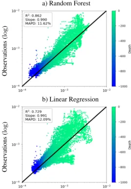
for the validation, very similar in shape and magnitude to the typical vertical profiles comprised in the training set. The scat-ter plot of measured vs. predictions for the NA dataset in Figure
7a shows a high R2of 0.86 for the RF algorithm and Figure7b
shows 0.73 for the RLR algorithm. The spread of the points appear to be for the lower depths (as for the test dataset in
Fig-ure4), and an overestimation on the surface. In Figure8a, the
STG displays a lower R2of 0.83 for the RF algorithm and
Fig-ure8b shows a higher R2 value of 0.86 for the RLR method.
The spread of the points on the 1:1 line is less compared with the NA; however, most of the points are situated above the line (constant overestimation) for the RF algorithm and below the line (constant underestimation) for the RLR algorithm. It is important to note that these validations show slight better or comparable statistics than the SOCA2016 independent
valida-tions for the NA and STG regions (R2 = 0.81and 0.85, slope
= 0.81 and 0.85 and Mean Absolute Percent Difference, MAPD = 12% and 21% for SOCA2016 in NA and STG, respectively;
see statistics for comparison with SOCA2020 in Figure8). As
SOCA2020 retrieves bbpwith a greatly improved depth
resolu-tion, this present work shows very promising results.
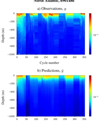
Figure9and Figure10show the comparison between in situ
measured and RF-estimated bbp time series for the two
valid-ation floats over the water column (from the surface to 1,000 m depth). Results from the predictions are fairly smooth
com-pared to the measured for the NA dataset (Figure9). Some of
the details near the surface cannot be reproduced with high de-tails in the predicted profile. Results from the predictions are
also smooth compared to the in situ measured bbpfor the STG
dataset (Figure10). The seasonal trend near the surface where
the bbpdecreases with time can be seen in both the predictions
and the measured values. The RF model reproduces well the
high bbpvalues up to the depth of the deep biomass maximum
(∼ 150-200 m) and then the bbpdecrease with depth from 200
m depth.
4. CONCLUSIONS
Preprocessing techniques and machine learning model presen-ted in this preliminary study give promising results, when using large datasets and attempting to predict a high number of output
layers. The overall performance statistics are quite good and bbp
vertical profiles present high similarities when compared with
in situobserved data. This is still ongoing work, so we expect
a) Random Forest Observ ations (log ) b) Linear Regression Observ ations (log )
Figure 7. The resulting statistics for the validation float in the North Atlantic (WMO=6901472). The top panel a) shows the results using the Random Forest algorithm and bottom b) the
results using the Linear regression. The y-axis are the observations (log-scale) and the x-axis are the predictions
(log-scale). The black line is the identity line. a) Random Forest Observ ations (log ) b) Linear Regression Observ ations (log )
Figure 8. The resulting statistics for the validation float in the South Atlantic Subtropical Gyre (WMO=3902121). The top panel a) shows the results using the Random Forest algorithm and bottom b) the results using the Linear regression. The y-axis are the observations (log-scale) and the x-axis are the predictions
North Atlantic, 6901486 a) Observations, y Depth (m) Cycle number b) Predictions, ˆy Depth (m)
Figure 9. The validation bbpprofiles (BGC-Argo float 6901486)
as a function of depth and cycles (time) for the North Atlantic
dataset. Panel a) shows the in situ bbpprofiles measured from the
float and panel b) shows the predictions from the Random Forest regressor model.
to see even better results (or at least more physically consistent) with algorithms and models adjusted to the several character-istics of the water column. Ultimately, using ML models to
in-crease predictions of bbpprofiles is a good endeavour and could
be a viable option when coupled with more physical constraints and validation. Eventually, derived uncertainties will also be tackled, which will require another family of methods not yet tested.
The results from the new method (SOCA2020) will be avail-able to users as part of the European Copernicus Marine Envir-onment Monitoring Service (CMEMS). More specifically, the 4-dimensional products of particulate organic carbon
(estim-ated from bbpusing the method ofCetinic et al.(2012)) will be
produced using merged hydrological and satellite (ocean color and altimetric) gridded-data available from CMEMS. The
res-olution of these products will be 0.25◦x0.25◦spatially, weekly
temporally (from January 1998 to December 2018) and at 19 depth levels vertically from the surface to 1,000 m depth. These resolutions are defined from the lower input products resolu-tions (i.e. physical data). In addition, a multi-year monthly climatology will be provided. These CMEMS products will be first released within the year 2020 and then will be updated yearly. As all CMEMS products, these products will be quali-fied against totally independent in situ observations.
One of the future perspective of the present study is to develop the same method as SOCA2020 to retrieve chlorophyll a con-centration, that is also a key biogeochemical product measured from profiling floats. The conjoint use of these two SOCA
methods (that will retrieve bbpand chlorophyll a concentration)
South Atlantic Subtropical Gyre, 3902121 a) Observations, y Depth (m) Cycle number b) Predictions, ˆy (m) Cycle number
Figure 10. The validation bbpprofiles (BGC-Argo float
3902121) as a function of depth and cycles (time) for the
Subtropical Gyre dataset. Panel a) shows the in situ bbpprofiles
measured from the float and panel b) shows the associated predictions from the Random Forest regressor model. would offer a new path to examine the variability in the phyto-plankton carbon to chlorophyll relationship over the vertical di-mension, which would represent a great opportunity for a bet-ter understanding of light and nutrient control of phytoplankton biomass and physiological status at a global scale. This is a cru-cial step for improving the characterization of the distribution and variability in ocean primary production and carbon export.
References
Bergen, K. J., Johnson, P. A., de Hoop, M. V., Beroza, G. C., 2019. Machine learning for data-driven discovery in solid Earth geoscience. Science, 363(6433).
Boyd, P. W., Claustre, H., Levy, M., Siegel, D. A., Weber, T., 2019. Multi-faceted particle pumps drive carbon sequestra-tion in the ocean. Nature, 568(7752), 327–335.
Briggs, N., Dall’Olmo, G., Claustre, H., In Press. Major role of
particle fragmentation in regulating sequestration of CO2by
the Oceans. Science.
Camps-Valls, G., Sejdinovic, D., Runge, J., Reichstein, M., 2019. A Perspective on Gaussian Processes for Earth Obser-vation. National Science Review, 6(4), 616-618.
Cetinic, I., Perry, M. J., Briggs, N. T., Kallin, E., D’Asaro, E. A., Lee, C. M., 2012. Particulate organic carbon and in-herent optical properties during 2008 North Atlantic Bloom Experiment. Journal of Geophysical Research, 117(C6), C06028.
Claustre, H., Johnson, K. S., Takeshita, Y., 2020. Observing the Global Ocean with Biogeochemical-Argo. Annual review of marine science, 12.
Dufois, F., Hardman-Mountford, N. J., Greenwood, J., Richard-son, A. J., Feng, M., Matear, R. J., 2016. Anticyclonic eddies are more productive than cyclonic eddies in subtropical gyres because of winter mixing. Science advances, 2(5), e1600282. Gardner, W., Mishonov, A., Richardson, M., 2006. Global POC concentrations from in-situ and satellite data. Deep Sea Re-search Part II: Topical Studies in Oceanography, 53(5-7), 718–740.
Garnesson, P., Mangin, A., Fanton d’Andon, O., Demaria, J., Bretagnon, M., 2019. The CMEMS GlobColour chlorophyll a product based on satellite observation: multi-sensor mer-ging and flagmer-ging strategies. Ocean Science, 15(3), 819–830. L´evy, M., Franks, P. J., Smith, K. S., 2018. The role of submesoscale currents in structuring marine ecosystems. Nature communications, 9(1), 1–16.
Loisel, H., Nicolas, J.-M., Deschamps, P.-Y., Frouin, R., 2002. Seasonal and inter-annual variability of particulate organic matter in the global ocean. Geophysical Research Letters, 29(24), 2196.
Malde, K., Handegard, N. O., Eikvil, L., Salberg, A.-B., 2019. Machine intelligence and the data-driven future of marine science. ICES Journal of Marine Science. fsz057.
Mignot, A., Claustre, H., Uitz, J., Poteau, A., D’Ortenzio, F., Xing, X., 2014. Understanding the seasonal dynamics of phytoplankton biomass and the deep chlorophyll maximum in oligotrophic environments: A Bio-Argo float investiga-tion. Global Biogeochemical Cycles, 28(8), 856–876. Reichstein, M., Camps-Valls, G., Stevens, B., Denzler, J.,
Carvalhais, N., Jung, M., Prabhat, 2019. Deep learning and process understanding for data-driven Earth System Science. Nature, 566, 195-204.
Roemmich, D., Alford, M. H., Claustre, H., Johnson, K., King, B., Moum, J., Oke, P., Owens, W. B., Pouliquen, S., Purkey, S. et al., 2019. On the future of Argo: A global, full-depth, multi-disciplinary array. Frontiers in Marine Science, 6. Roemmich, D., Johnson, G., Riser, S., Davis, R., Gilson, J.,
Owens, W. B., Garzoli, S., Schmid, C., Ignaszewski, M., 2009. The Argo Program: Observing the Global Oceans with Profiling Floats. Oceanography, 22(2), 34–43.
Ruescas, A. B., Hieronymi, M., Mateo-Garcia, G., Koponen, S., Kallio, K., Camps-Valls, G., 2018. Machine Learning Regression Approaches for Colored Dissolved Organic Mat-ter (CDOM) Retrieval with S2-MSI and S3-OLCI Simulated Data. Remote Sensing, 10(5).
Sauz`ede, R., Claustre, H., Uitz, J., Jamet, C., Dall’Olmo, G., D’Ortenzio, F., Gentili, B., Poteau, A., Schmechtig, C., 2016. A neural network-based method for merging ocean color and Argo data to extend surface bio-optical properties to depth: Retrieval of the particulate backscattering coefficient. Journal of Geophysical Research: Oceans, 121(4), 2552– 2571.
Schmechtig, C., Poteau, A., Claustre, H., D’Ortenzio, F., Dall’Olmo, G., Boss, E., 2016. Processing Bio-Argo particle backscattering at the DAC level. Argo data management. Stramska, M., 2009. Particulate organic carbon in the global
ocean derived from SeaWiFS ocean color. Deep Sea Re-search Part I: Oceanographic ReRe-search Papers, 56(9), 1459– 1470.
Stramski, D., Reynolds, R. A., Babin, M., Kaczmarek, S., Lewis, M. R., R¨ottgers, R., Sciandra, A., Stramska, M., Twardowski, M. S., Franz, B. A., Claustre, H., 2008. Re-lationships between the surface concentration of particulate organic carbon and optical properties in the eastern South Pa-cific and eastern Atlantic Oceans. Biogeosciences, 5(1), 171– 201.
Xu, D., Shi, Y., Tsang, I. W., Ong, Y., Gong, C., Shen, X., 2019. Survey on Multi-Output Learning. IEEE Transactions on Neural Networks and Learning Systems, 1-21.
´
Alvarez, M. A., Rosasco, L., Lawrence, N. D., 2012. Kernels for Vector-Valued Functions: A Review. Foundations and
Trends in Machine Learning, 4(3), 195-266.R
ACKNOWLEDGEMENTS
This work has been (partly) funded by the European “Coper-nicus Marine Environment Monitoring Service” and partially funded by the European Research Council (ERC) under the ERCCoG-2014 SEDAL project (grant agreement 647423), ERCAdG-2010 remOcean project (grant agreement 246577) and ERCAdG-2019 REFINE project (grant agreement 834177).