HAL Id: insu-01356011
https://hal-insu.archives-ouvertes.fr/insu-01356011
Submitted on 24 Aug 2016
HAL is a multi-disciplinary open access archive for the deposit and dissemination of sci-entific research documents, whether they are pub-lished or not. The documents may come from teaching and research institutions in France or abroad, or from public or private research centers.
L’archive ouverte pluridisciplinaire HAL, est destinée au dépôt et à la diffusion de documents scientifiques de niveau recherche, publiés ou non, émanant des établissements d’enseignement et de recherche français ou étrangers, des laboratoires publics ou privés.
I Panet, F Pollitz, V Mikhailov, M Diament, P Banerjee, K Grijalva
To cite this version:
I Panet, F Pollitz, V Mikhailov, M Diament, P Banerjee, et al.. Upper mantle rheology from GRACE and GPS postseismic deformation after the 2004 Sumatra-Andaman earthquake. Geochemistry, Geo-physics, Geosystems, AGU and the Geochemical Society, 2010, 11 (6), pp.10.1029/2009GC002905. �10.1029/2009GC002905�. �insu-01356011�
Click Here for
Full Article
Upper mantle rheology from GRACE and GPS postseismic
deformation after the 2004 Sumatra
‐Andaman earthquake
I. Panet
Laboratoire de Recherche en Géodésie, Institut Géographique National, ENSG, 6/8, avenue Blaise Pascal, Cité Descartes, Champs/Marne, F‐77455 Marne‐la‐Vallée CEDEX 2, France
Also at Institut de Physique du Globe de Paris, Université Paris‐Diderot, CNRS, 35, rue Hélène Brion, F‐75205 Paris CEDEX 13, France
F. Pollitz
U.S. Geological Survey, 345 Middlefield Road, MS 955, Menlo Park, California 94025‐3591, USA ([email protected])
V. Mikhailov
Institut de Physique du Globe de Paris, Université Paris‐Diderot, CNRS, 35, rue Hélène Brion, F‐75205 Paris CEDEX 13, France
Also at Institute of Physics of the Earth, Russian Academy of Science, B. Gruzinskaya 10, Moscow 123810, Russia ([email protected])
M. Diament
Institut de Physique du Globe de Paris, Université Paris‐Diderot, CNRS, 35, rue Hélène Brion, F‐75205 Paris CEDEX 13, France ([email protected])
P. Banerjee
Earth Observatory of Singapore, Nanyang Technological University, 50 Nanyang Drive, 639798 Singapore
K. Grijalva
Berkeley Seismological Laboratory, University of California, 307 McCone Hall, Berkeley, California 94720‐4767, USA
[1] Mantle rheology is one of the essential, yet least understood, material properties of our planet,
control-ling the dynamic processes inside the Earth’s mantle and the Earth’s response to various forces. With the advent of GRACE satellite gravity, measurements of mass displacements associated with many processes are now available. In the case of mass displacements related to postseismic deformation, these data may provide new constraints on the mantle rheology. We consider the postseismic deformation due to the Mw= 9.2 Sumatra 26 December 2004 and Mw= 8.7 Nias 28 March 2005 earthquakes. Applying wavelet
analyses to enhance those local signals in the GRACE time varying geoids up to September 2007, we detect a clear postseismic gravity signal. We supplement these gravity variations with GPS measurements of postseismic crustal displacements to constrain postseismic relaxation processes throughout the upper mantle. The observed GPS displacements and gravity variations are well explained by a model of visco-elastic relaxation plus a small amount of afterslip at the downdip extension of the coseismically ruptured
body rheology. The mantle below depth 220 km has a Maxwell rheology. Assuming a low transient vis-cosity in the 60–220 km depth range, the GRACE data are best explained by a constant steady state vis-cosity throughout the ductile portion of the upper mantle (e.g., 60–660 km). This suggests that the localization of relatively low viscosity in the asthenosphere is chiefly in the transient viscosity rather than the steady state viscosity. We find a 8.1018Pa s mantle viscosity in the 220–660 km depth range. This may indicate a transient response of the upper mantle to the high amount of stress released by the earthquakes. To fit the remaining misfit to the GRACE data, larger at the smaller spatial scales, cumulative afterslip of about 75 cm at depth should be added over the period spanned by the GRACE models. It produces only small crustal displacements. Our results confirm that satellite gravity data are an essential complement to ground geodetic and geophysical networks in order to understand the seismic cycle and the Earth’s inner structure.
Components: 11,500 words, 11 figures, 1 table.
Keywords: satellite gravity; mantle rheology; seismic cycle.
Index Terms: 1217 Geodesy and Gravity: Time variable gravity (7223); 1236 Geodesy and Gravity: Rheology of the lithosphere and mantle (7218); 1242 Geodesy and Gravity: Seismic cycle related deformations (6924).
Received 20 October 2009; Revised 18 March 2010; Accepted 26 March 2010; Published 19 June 2010.
Panet, I., F. Pollitz, V. Mikhailov, M. Diament, P. Banerjee, and K. Grijalva (2010), Upper mantle rheology from GRACE and GPS postseismic deformation after the 2004 Sumatra‐Andaman earthquake, Geochem. Geophys. Geosyst., 11, Q06008, doi:10.1029/2009GC002905.
1. Introduction
[2] Knowing crustal and mantle rheology is
essential for understanding how the Earth behaves when it is subject to a stress and what processes operate in its deep interior. In particular, mantle viscosity is one of the most important, yet least understood, properties of the inner Earth, control-ling mantle dynamics and the pattern of convective flows. It exerts a first‐order control on tectonic plates velocities, on the Earth’s deformation in response to transient forces and loads (e.g., coseismic stress steps), and on stress distribution in subduction zones. In addition to laboratory experiments, geo-physical observations have been used as probes of the mantle rheology at various spatial and temporal scales [e.g., Hager, 1991; King, 1995]. These include observations of geoid and crustal uplift following the last deglaciation, observations of postseismic deformation, models of geoid and dynamic topography using the density structure derived from seismic tomography, and tectonic plate velocities. Because of the difficulty of inter-preting laboratory experiments under real mantle conditions, direct observations of the Earth’s vis-cous deformation are very important. Geophysi-cally inferred viscosity models typiGeophysi-cally depend on elapsed time since the forcing event and on the size
of the source. Additional assumptions may be needed, such as an ice sheet model in the case of postglacial rebound, or a seismic velocity/density model to interpret the large‐scale geoid. With the recent advent of satellite gravity, a new observation technique has become available to quantify Earth’s deformation in response to different loads, through the detection and analysis of their gravity sig-natures and their evolution in time. In the case of postseismic deformation, which involves relatively short observations and well‐known seismic sources, these new data may contribute to a better under-standing of mantle rheology.
[3] One of the largest earthquakes in recent
dec-ades, the Mw 9.2 Sumatra‐Andaman earthquake,
occurred on 26 December 2004 at a particularly complex subduction boundary, along which the Indian and Australian plates subduct below a set of microplates comprising the fore‐arc sliver plate, the Burma and the Sunda microplates [Ammon et al., 2005; Banerjee et al., 2005; Lay et al., 2005; Vigny et al., 2005]. In this area, the highly het-erogeneous oceanic plate subducts below a highly heterogeneous overriding plate, following an oblique direction of convergence [Diament et al., 1992; Deplus et al., 1998; Deplus, 2001; Curray, 2005]. The Sumatra‐Andaman earthquake rup-tured at least 1300 km of this subduction boundary,
causing a devastating tsunami. It was followed by numerous aftershocks and by a second very large earthquake, the Mw8.7 Nias earthquake, on 28 March
2005 (Figure 1). During the following years, slip at depth has continued, as evidenced by the sequence of recorded aftershocks.
[4] Owing to monitoring networks on the ground
(GPS stations, seismometry, tide gauges) and sat-ellite data (ionospheric perturbations, altimetry, satellite gravity), the Sumatra earthquakes are among the best monitored ever, providing a unique opportunity to understand the processes operating in the seismic cycle. For the very first time, the
Figure 1. Rupture areas associated with known megathrust earthquakes along the Sumatra‐Sunda trench. Black planes are the coseismic rupture of the 26 December 2004 earthquake from Model C of Banerjee et al. [2007]. Gray planes are the afterslip planes of this study. The six southern, thicker planes are the coseismic and postseismic fault planes for the Nias earthquake modeling. Indicated are the 0 and 50 km slab depth contours of Gudmundsson and Sambridge [1998]. Epicenters of earthquakes of magnitude larger than 4 from 29 March 2005 to 1 August 2005 from the NEIC catalog are superimposed. Selected GPS sites from three regional networks are indicated. The two brown stars correspond to the epicenters of the Sumatra‐Andaman December 2004 and Nias March 2005 earthquakes. The three blue boxes are the three areas of interest studied in the paper: the trench area (90°E–95°E, 4°N–9°N), the Nias area (93°E–98°E, 2°S–3°N) and the Thailand area (102°E–104°E, 4°N–6°N).
earthquakes has been measured at a global scale by GRACE satellite gravity [Han et al., 2006]. Launched in March 2002, the GRACE mission gives access to the temporal variation of the gravity field at a spatial resolution of about 400 km, and a temporal resolution from 10 days to 1 month. These variations are dominated by the effect of the water circulation between the atmosphere, the oceans, the land hydrological systems, and the polar ice caps. Such mass redistributions cause geoid variations of a few millimeters at various temporal and spatial scales [Dickey et al., 1997; Wahr et al., 1998]. Locally, large seismic events also generate geoid variations of the same amplitude, which may also be detectable by GRACE [Gross and Chao, 2001; Mikhailov et al., 2004; Sun and Okubo, 2004; de Viron et al., 2008].
[5] An important coseismic gravity decrease in the
Andaman Sea has been observed in the GRACE data for the 2004 Mw9.2 earthquake, followed by a
positive rebound [e.g., Han et al., 2006; Panet et al., 2007; Ogawa and Heki, 2007; Han et al., 2008; de Linage et al., 2008]. This gravity varia-tion is due to vertical displacement of density interfaces (mostly the upper crust boundary and the Moho), and to rock density changes resulting from variations of the stress field (dilatation/compression). At large scales, the density variation effect dom-inates that of the vertical displacement. The observed coseismic gravity low demonstrated how sensitive GRACE was to the contribution of dila-tation/compression of lithosphere and mantle rocks [Han et al., 2006]. Part of the gravity low has been attributed to nonuniform coseismic subsidence of the Andaman Sea overriding plate [Panet et al., 2007]. A postseismic gravity increase has been observed by GRACE around the Sumatra trench since 2005, and this has been related to viscoelastic relaxation or mantle water diffusion [Panet et al., 2007; Ogawa and Heki, 2007; Han et al., 2008; de Linage et al., 2008]. The effect of the post-seismic processes on the low degrees of GRACE gravity solutions was detected and discussed in terms of viscoelastic relaxation by Cannelli et al. [2008].
[6] Here, we study the postseismic gravity signal
from almost 3 years of GRACE data, until the end of 2007, and combine it with surface GPS mea-surements in order to derive a model for post-seismic deformation that fits both the GPS and the GRACE data. Analyzing the variability of the signal at different spatial scales with wavelets, we
but cannot explain all the gravity variations. The viscoelastic relaxation model that best fits the GPS measurements of crustal displacement for the first 3 years is a modification of the model presented by Pollitz et al. [2006a] based on the first year. This viscoelastic relaxation has to be combined with a small amount of afterslip at depth, below the coseismically ruptured area, in order to fit the sat-ellite gravity data. Finally, we discuss the geody-namic implications of our findings.
2. Data Processing
2.1. GRACE Geoids
[7] We analyzed the Release 1 of the decadal
geoids by Biancale et al. [2007], hereafter referred to as GRGS geoids, spanning the period between August 2002 and September 2007, computed from the GRACE satellites measurements. These geoids are provided in the form of spherical harmonic coefficients of the geopotential up to degree 50 (resolution 400 km) on the Web site of the Bureau Gravimétrique International (http://www.geodesie. ird.fr/bgi). They are computed by a regularized least squares inversion of the measurements. The regularization toward a mean static gravity field is applied for the spherical harmonic degrees larger than about 30 [Lemoine et al., 2007], the lower degree harmonics being unconstrained. Back-ground geophysical models are used to correct the raw measurements from the high frequency vari-ability associated with atmospheric pressure varia-tions, ocean circulation and tides, in order to limit their aliasing in the geoid solutions. The geoid solutions that we analyze finally contain signals related to the water mass circulation between con-tinents, polar ice caps and oceans, and solid Earth geoid variations including earthquake signals. The errors in the background models, and the unmodeled high‐frequency signals, map into longitudinal, north‐south elongated errors in these geoids. Some of these errors may be due to long‐period noise. Oceanic tide aliasing effect, in particular, may be noticeable in the polar, coastal and shallow oceanic regions, with periodicities 161 days, 3.7 and 7.5 years [Ray and Luthcke, 2006]. Geoid variations of about 0.5 mm over periods larger than 3 months may result from errors in the ocean tide models [Schrama and Visser, 2007].
[8] To remove the water cycle signal, characterized
adjusted and removed a 161 day, a semiannual, and an annual cycle. To avoid the leakage of the earthquake coseismic signal in these estimates, a step function at the time of the Sumatra‐Andaman earthquake (26 December 2004) was simulta-neously fitted, but not removed from the geoid signal. We also tried to fit a possible 3.7 year tide alias in the area, but our estimates were biased by the large postseismic gravity variations.
2.2. Spatiotemporal Analysis of the GRACE Geoids
[9] To enhance the earthquake signal (resulting
from both coseismic and postseismic processes) in the GRACE data, we combine a multiscale filtering of the geoids in the space domain with an averag-ing in the time domain, over various time spans. This allows us to extract the earthquake signal without making assumptions about its temporal variability, such as an exponential decay. Given the complexity and the large number of earthquakes that occurred in this area since 2005, the time dependence of the signal may indeed be rather complex.
[10] Gravity variations caused by earthquakes have
a characteristic scale of the size of the ruptured area, 1300 km in the case of the Sumatra 2004 main earthquake. They are mixed in with noise: large‐ and medium‐scale patterns due to the geo-fluid signals remaining (water mass displacements due to interannual and long‐term variability of continental hydrology and oceanic circulation), and small‐scale patterns due to the striped noise resulting from the aliasing effects in GRACE geoid solutions. To enhance and extract the earthquake signal from GRACE models, we thus applied a multiscale filtering of the geoids based on a con-tinuous wavelet analysis (CWT). A wavelet is a function well localized both in space and frequency, characterized by a scale parameter (describing its spectral coverage) and a position parameter (local-izing the spatial point around which it concentrates most of its energy). In this study, as in the works by Panet et al. [2006, 2007], we use the Poisson mul-tipole wavelets [Holschneider et al., 2003]. They are well suited for potential field analyses since they may be identified with multipolar sources located within the Earth. The reader interested in the wave-let theory and the continuous wavewave-let analyses is referred to Holschneider [1995] for more details; here we only recall a few basic ideas.
correlation coefficients between the GRACE geoids and wavelets at positions continuously sampling the area under study. The map of those correlation (CWT) coefficients identifies structures in the geoid at the wavelet scale considered. We then repeat the analysis at different scales. Because a constraint is applied in the computation of the GRGS geoids from the GRACE data at resolutions smaller than about 600 km, the geoids may underestimate the small‐ scale gravity variations from the earthquakes. Con-sequently, we do not investigate wavelet scales smaller than 600 km in our analysis. Then, studying the temporal variability of the highlighted structures at different scales allows a better understanding of the physical processes involved.
[12] To study the temporal variability of the geoid
components at different scales, and enhance those related to the Sumatra earthquakes, we stack the CWT coefficients over various time spans and remove the contribution of a reference geoid. We obtain so‐called “residual” geoid and CWT coef-ficients. Our reference geoid is the average geoid over the period from the beginning of January 2005 to the end of March 2005. It includes the coseismic signal from the Sumatra‐Andaman 2004 earth-quake and the first 3 months of postseismic deformation. Stacking to produce this reference geoid indeed allows us to lower its noise level (in particular due to the stripes). The price to pay when doing so is that one cannot study the early post-seismic relaxation. Then, the CWT of this reference geoid was subtracted from the CWT of the geoids stacked over longer periods starting in April 2005, allowing us to analyze the residual geoid signal. As the stack length increases, the remaining periodic and high frequency variability averages out, whereas the long‐term signals appear more clearly. This allows us to highlight the postseismic gravity variations in the Sumatra subduction zone. Note that possible temporal trends in geofluid signals will also be enhanced in this analysis. Their sepa-ration from the geodynamic signal is then based on their different spatial characteristics.
[13] Finally, we estimated the precision of the
CWT of our stacked geoids. For that, we used the calibrated errors on the spherical harmonic coeffi-cients provided with the GRGS geoids, and applied band‐pass filters defining the wavelets at different scales. We then computed the cumulative RMS errors up to degree 50. We thus obtained a formal CWT error at different wavelet scales, which
at 1000 km scale, and 0.3 mm at 1400 km scale for the 10 day geoids. For a monthly geoid, the pre-cision becomes 0.3 mm at 600 km scale, 0.23 mm at 1000 km scale and 0.17 mm at 1000 km scale. These results are consistent with a noise estimation carried out by de Viron et al. [2008]. They compared the GRGS Release 1, GFZ and CSR monthly geoids and estimated their variance using the tricornered hat method. The GFZ geoids are computed from the GRACE data by the GeoForschungsInstitut (Potsdam, Germany), and the CSR geoids are computed by the Center for Space Research, Austin, Texas. De Viron et al. [2008] concluded that a 0.3 mm precision for the monthly geoids at 400 km resolution was a reasonable estimate. This corre-sponds to our higher error boundary, for a wavelet‐ filtered solution. Finally, when we simply consider the monthly variability of the CWT of the GRGS geoids in a wide area around Sumatra, we again find similar amplitudes of variations, not attributable to the earthquake signals. We thus conclude that our CWT error estimates are acceptable and may slightly overestimate. Then, the RMS errors of the CWT of the reference geoid (3 month stack) reaches 0.14 mm, 0.11 and 0.08 mm at 600, 1000 and 1400 km scales, respectively. For a stack from April 2005 until September 2007, it amounts to 0.04, 0.03 and 0.02 mm. When we remove the reference geoid from the stacks over different periods, we should add the error on this reference geoid to the error of the stacked geoid, leading to an error estimate of the residual geoid of about 0.28, 0.22 and 0.16 mm for the stacks up to June 2006, and 0.18, 0.14 and 0.1 mm for the stacks up to September 2007. As the same constant reference field is subtracted from all stacks, its error does not impact the growth rate of the stacked signal in the following years. The precision of the growth rate is limited by the pre-cision of the stacks, without adding the reference geoid error.
2.3. GPS Data
[14] To enhance our postseismic deformation
models, we analyzed surface GPS measurements in addition to the GRACE gravity data. We have compiled data from five sites belonging to several continuously operating GPS networks, including: the Thai Geodetic Network (THAI), the National Institute of Information and Communications Technology (NICT), and the International GPS Service (IGS). The GPS sites are located in Thailand and Singapore, in the back‐arc region of the Sunda
processed with the GAMIT/GLOBK software package [Herring et al., 2008a, 2008b] to produce time series of station coordinates in the ITRF‐2000 reference frame [Altamimi et al., 2002]. We used a minimum of 15 global IGS GPS stations to implement the ITRF‐2000 reference frame. The stations used to determine the reference frame are more than 1600 km from the Sumatra‐Andaman earthquake rupture. The GPS data yielded 2‐D horizontal displacements that span the time period between January 2005 and June 2008. Background interseismic motions, estimated from a regional relative plate motion model (E. V. Apel et al., Indian plate motion, deformation and plate boundary interactions, submitted to Geophysical Journal International, 2010), have been removed from the postseismic time series. The interseismic motions are predominantly eastward and vary in magnitude between 2.9 cm/yr at NTUS to 3.4 cm/yr at BNKK, with 1 sigma uncertainties for both horizontal components of up to 0.2 cm/yr. In this study, we do not use vertical GPS displacements, because this component is the least precisely measured by GPS, whereas satellite gravity is particularly sensitive to its impact on the gravity field.
3. Results
[15] Figure 2 represents the CWT at 600 km, 1000 km
and 1400 km scales of the residual geoids stacked from April 2005 to March 2006 (Figure 2, top), and from April 2005 to September 2007 (Figure 2, bottom). Figures S1–S3 in the auxiliary material show a larger number of stacking intervals, also showing the reference geoid.1 The dominant tem-poral signal is a clear gravity increase along the trench, likely to be a postseismic signal given its shape and location around the subduction zone. This kind of signal was already observed by Panet et al. [2007], Han et al. [2008], and de Linage et al. [2008] and is confirmed by the present analysis. The geoid growth reaches the millimeter level at the scales investigated. The coseismic gravity var-iation due to the Nias 28 March 2005 earthquake also appears clearly, in particular at the 600 km scale. It is associated with to a gravity increase around the location (2°S, 97°E). Aside from these positive anomalies, we note two negative
anoma-1Auxiliary materials are available in the HTML. doi:10.1029/
lies of the geoid, the first in the Indian Ocean and the second around Thailand. The time dependence of the gravity variation in Thailand is not mono-tonic, as shown in Figure 3, in contrast to what is expected in the case of a postseismic relaxation. This suggests that residual geofluid signals in this area are likely to overprint a possible geodynamic signal. Han and Simons [2008] separated the earthquake coseismic signal from an important seasonal hydrology cycle, and an analysis of oce-anic and hydrological models by de Linage et al. [2008] supports a possible long‐term geofluid sig-nal there. Consequently, we conclude that an important part of the anomaly over Thailand is not of geodynamic origin, even if the final model con-structed in this paper partly explains the minima observed. Finally, we also observe a persistent nega-tive anomaly in the Indian Ocean, around location 5°S, 92°E). Because of its monotonic evolution in time, and its location close to the maximum of anomaly, it may be related to the growth of the
earthquake postseismic signals. Indeed, viscoelastic models studied in the remainder of this paper also show a negative anomaly in this area.
[16] Figure 3 shows the growth of the CWT
coef-ficients represented in Figure 2, in three significant locations: the trench area (between 91°E–93°E and 7°N–9°N), the Nias area (between 96°E–98°E and 1°S–1°N), and the Thailand area (between 102°E– 104°E and 4°N–6°N). The growth of the signal is studied only for stacking periods larger than 3 months (June 2005), otherwise the noise level would be too high. Consequently, the growth of the signal is plotted with respect to the value of the June 2005 stack. In the trench and Nias area, we observe that the growth rate of the geoid anomalies is larger as the scale increases. In the trench area, the growth of the 600 km scale com-ponent slows down after June 2006, whereas the 1400 km scale anomaly keeps increasing continu-ously. In the Nias area, we note that the 1400 km scale anomaly becomes noticeably larger than the
Figure 2. Wavelet analyses of the stacked geoids at (left) 600 km scale, (middle) 1000 km scale, and (right) 1400 km scale. The reference geoid has been subtracted for all plots. (top) A stack from April 2005 to March 2006. (bottom) The stack from April 2005 to September 2007.
This suggests a propagation of the postseismic sig-nal from the Sumatra‐Andaman 2004 earthquake in the Nias area. Finally, even if it is much noisier, the Thailand anomaly evolution is consistent with a postseismic signal, at first order.
4. Postseismic Deformation Models
[17] Different processes may be invoked to explain
the observed signal. Given the large size of the earthquake, viscoelastic relaxation of stress changes in the mantle would be expected to play an important role after the earthquake [Pollitz et al., 2006a]. At the rather large spatial scales resolv-able by GRACE, it is likely to be a dominant contribution. Afterslip was also suggested by a few studies [Vigny et al., 2005; Hashimoto et al., 2006; Chlieh et al., 2007; Paul et al., 2007]. Indeed, the large number of aftershocks and the sequence of earthquakes that occurred during the years 2005 to 2007 indicate slip at depth during this period. However, afterslip is a smaller‐scale process as compared to viscoelastic relaxation, as will be con-firmed in this study. Finally, poroelastic rebound in the crust may also occur after the earthquake [Masterlark et al., 2001]. The associated time scale is usually too short and the affected area too local to explain our observations. More recently, Ogawa and Heki [2007] have suggested that supercritical water diffusion may take place in the mantle and compensate for coseismic dilatation/compression for the Sumatra earthquake, but they do not pro-vide any modeling of the geoid variations caused by this process. Thus, as a first approximation, we do not consider this possible effect in our modeling explicitly. However, the presence of water in the crust and mantle is expected to affect the rheology by generally reducing viscosity [e.g., Bürgmann and Dresen, 2008].
4.1. Viscoelastic Deformation Model
[18] First, we compared the GRACE data with the
predictions of a viscoelastic relaxation model out-put of the Sumatra‐Andaman 2004 and the Nias 2005 earthquakes. This model is the one that best
over the year 2005 [Pollitz et al., 2006a], and is referred to as the VE06 model in this paper. The source models described by Banerjee et al. [2007] are constrained from GPS static offsets corrected for postseismic motions to the time 1 day following the earthquake. This duration has been chosen to account for the whole coseismic signal without introducing too much postseismic signal. For the 2004 earthquake, the model has between 2 and 19 m of slip (average slip is about 10 m) on a 1300 km long, 100/140 km wide set of fault planes (Mw9.2). For the Nias March 2005 event, it
corresponds to an earthquake of magnitude Mw =
8.66, a value larger than the magnitudes inferred from seismology. From these source models, we compute the stress and strain distribution resulting from the earthquake, and the consequent visco-elastic postseismic relaxation in a spherically symmetric Earth, with elastic layering according to the PREM model [Dziewonski and Anderson, 1981]. It consists of a 60 km thick lithosphere overlying a 160 km thick asthenosphere with a biviscous Burgers body rheology. A Burgers body exhibits an early Kelvin solid behavior (viscously damped elastic deformation) and a long‐term Maxwell fluid behavior, to which correspond the transient and steady state viscosities, respectively. Thus, it allows to linearly model an asthenospheric response with more than one characteristic relaxa-tion time, related to the presence of weak inclu-sions, transient creep or nonlinear flow [Pollitz, 2003]. Here, the transient and steady state viscosi-ties in the asthenosphere (depth range 60 to 220 km) are 5 · 1017 Pa s and 1019 Pa s. The mantle below depth 220 km has a Maxwell rheology with higher viscosity (1020 Pa s for the upper mantle and 1021Pa s for the lower mantle). Coseismic and viscoelastic postseismic relaxation are computed with the methods of Pollitz [1996, 1997]. Corresponding geoid variations are derived, taking into account surface deformation and stress‐ induced density variations (dilatation), as explained by Panet et al. [2007]. The spherical harmonic expansion of these geoid variations is truncated up to degree 50 and order 50 to ensure consistency with the GRACE data. Figure 4 represents the
Figure 3. Temporal growth of the CWT coefficients of the residual geoids with respect to the value of June 2005 (month 6). The residual geoids are stacked from April 2005 (month index 4) for all the stacking intervals starting from June 2005 (month 6) up to September 2007 (month 33) for three locations. (a) The trench (maximum of anomaly in the area 90°E–95°E, 4°N–9°N), (b) the Nias area (maximum of anomaly in the area 93°E–98°E, 2°S–3°N), and (c) the Thailand area (average for the area 102°E–104°E, 4°N–6°N). Black curves indicate 600 km scale, red curves indicate 1000 km scale, and green curves indicate 1400 km scale.
CWT of the geoid variations up to degree 50, computed from this model stacked from April 2005 to September 2007, and Figure 5 compares, in the trench area (between 91°E–93°E and 7°N–9°N), the growth of the modeled signal (red curves) with the observed one (black curves).
[19] The observed geoid variations are larger and
cover broader areas than the modeled ones: the model lacks energy as compared with the observa-tions, as also seen by Simons et al. [2009] with a purely elastic modeling. This observation holds especially for the larger‐scale components, for which the observed GRACE variations have much larger amplitude than the modeled ones. Such large‐scale components are not well constrained by the GPS data used to construct the relaxation model: indeed, their spatial distribution is sparse, and the precision of the vertical displacements is the lowest, whereas gravity is, in contrast, very sensitive to the vertical displacement of the crust. Moreover, GPS measurements are much less sen-sitive than GRACE data to the deeper processes affecting the whole upper mantle. Thus, the anal-ysis of the GRACE data brings complementary information, and suggests either that another pro-cess, such as afterslip, has to be introduced to account for part of the observations, and/or that we need to modify the viscoelastic relaxation model. Afterslip is not likely to generate the largest signal at the largest scale (and this will be confirmed later in this paper), so we first modified the viscosity profile of the viscoelastic model.
[20] Modifying the viscosity in the lower mantle
does not improve the fit to the data because rather
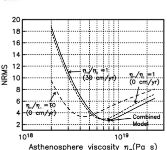
high viscosities are involved and their impact on the 3 year geoid variation is too small to be clearly detectable at GRACE precision. The biviscous rheology in the asthenosphere is suggested by many earthquake studies [Pollitz et al., 1998, 2001; Pollitz, 2003], so we kept the Burgers body model for the asthenosphere. Tests show that modifying the asthenospheric rheology (the transient viscosity, steady state viscosity, or transient shear modulus) cannot match the long‐wavelength GRACE data without seriously compromising the fit to the GPS data. The sensitivity of predicted GPS motions to steady state asthenosphere viscosity is indeed demonstrated by viscoelastic relaxation models, with or without afterslip added, where this viscosity is systematically varied and its influence on result-ing fits to surface displacement is evaluated. Letha
and hm be the steady state mantle viscosity in the
depth range 60–220 km and 220–670 km, respec-tively. Figure 6 shows the pattern of normalized root‐mean‐square (NRMS) misfit between the observed and calculated GPS time series as a function of ha, assuming two values for the ratio
hm/ha. It indicates that steady state asthenosphere
viscosity must be close to 8 · 1018Pa s (as indicated by the filled circle in Figure 6) in order to satisfy the GPS data.
[21] The rheology of the mantle below the
asthenosphere is less known, and the GRACE data bring here valuable constraints. Note that Figure 6 shows that the GPS measurements are moderately sensitive to the viscosity of the deeper layers (below 220 km depth). A comparison of the results withhm/ha= 10 and those withhm/ha= 1 in Figure 6
indicates that GPS data misfit is lower for the latter
Figure 4. CWT at (left) 600 km, (middle) 1000 km, and (right) 1400 km scales of the geoid variations up to spher-ical harmonic degree 50 predicted from the model by Pollitz et al. [2006a], for the Nias March 2005 coseismic and postseismic viscoelastic deformation and the Sumatra‐Andaman December 2004 postseismic viscoelastic deforma-tion. The stacking applied is from April 2005 to September 2007.
ratio. The GPS data thus suggest that the viscosity value in the 220–670 km layer is substantially less than the 1020 Pa s value used in the VE06 model (Table 1), and the GRACE geoid data provide a stronger test of this hypothesis.
[22] To illustrate the sensitivity of the GRACE data
tohm, Figure 7 shows the geoid effect of a viscosity
change from 1020Pa s to 1019Pa s. It decreases the positive signal along the trench at small scales, and slightly increases the largest‐scale components (see also Table 1). We note that a significant decrease of the viscosity is needed in order to improve the fit to the GRACE data. Keeping the ratiohlm/haconstant,
wherehlmis the lower mantle viscosity, we obtain
the best results by decreasing hm to 8.1018 Pa s
(model VEB1 of Table 1). Such a low value is not
gravity variation at a characteristic time constant of 2–3 years, which is consistent with the obtained value of the viscosity. What GRACE shows is that a viscosity value near 1019Pa s cannot be limited to the superficial layers, but must exist in a larger volume affecting the whole upper mantle. Note that the suggested viscosity decrease also damps the Thailand and Indian Ocean anomalies. However, as they are the noisier part of the observations, we prefer to constrain the model mostly from the geoid variations in the trench area. We find that visco-elastic relaxation on model VEB1 is sufficient to explain the joint GPS/GRACE data sets at all scales, provided that viscoelastic relaxation is appended with afterslip at depth, which we explore in section 4.2.
4.2. Afterslip Model
[23] To show that the remaining misfits of the
geoid profiles are well explained by afterslip, we calculated the geoid variations caused by afterslip at depth. To model it, we assume steady afterslip taking place on the 100 km downdip continuation of the upper (0–30 km depth) coseismic fault planes by Banerjee et al. [2007]. Our afterslip fault planes have depth of the upper edge equal to 30 km, depth of the lower edge equal to 87.4 km, and dip angle 35°. These afterslip fault planes are represented in Figure 1. Our afterslip model has a very simple linear time dependence. Indeed, the relatively low spatial resolution of the GRACE data and the trade‐off with viscoelastic relaxation limits the precision of the afterslip model. We can only constrain the net amount of afterslip accumulated during the period spanned by our data. We tried different cumulative amounts of slip at depth. This confirmed that it is not possible to fit the GRACE data with afterslip only, because the scale depen-dence of the anomaly cannot be respected (see Table 1).
[24] The remaining geoid misfits are well modeled
by 75 cm of slip over the studied period, corresponding to an average rate of 30 cm/yr. This cumulative afterslip corresponds to an earthquake of magnitude approximately equal to Mw= 8.2. This
is comparable with the estimates of Hashimoto
Figure 5. CWT at (a) 600 km, (b) 1000 km, and (c) 1400 km scales of the geoid variations stacked from April 2005 for the GRACE data (black curves), the reference VE06 relaxation model from Pollitz et al. [2006a] (red curves), the VEB1 relaxation model (green curves), the 30 cm/yr afterslip model (blue curves), and the hybrid VEB1 relaxation model with 30 cm/yr afterslip added (pink curves). The values correspond to the location of the maximum of the positive anomaly in the trench area between 90°E and 95°E, 4°N and 9°N.
Figure 6. NRMS of observed GPS time series (Figure 10) with respect to a Burgers body viscoelastic relaxation model as a function of steady state asthenosphere viscos-ityhafor two values of the ratiohm/ha, wherehaandhm
are the steady state mantle viscosity in the depth ranges 60–220 km and 220–670 km, respectively; the ratios ha/h2= 20 andhlm/ha= 100 are assumed, whereh2is
the transient viscosity in the depth range 60–220 km andhlmis the lower mantle viscosity. For the case where
hm/ha= 10, afterslip rate is assumed to be zero; for the
case wherehm/ha= 1, misfit results are shown for
after-slip rates of 0 and 30 cm/yr. The filled circle indicates the“combined model” (combined relaxation VEB1 and afterslip model described in section 4, i.e., with viscos-ity parameters given in Figure 11 (solid profile) and afterslip rate of 30 cm/yr).
et al. [2006], which show that the first 3 months of afterslip (shallow in their model) following the Sumatra‐Andaman 2004 earthquake are equivalent to a Mw8.7 earthquake. If afterslip takes place at a
shallow depth, then the associated geoid pattern is similar to the observed GRACE coseismic varia-tions: mostly a geoid decrease in the Andaman Sea. If afterslip takes place at deeper depth, the geoid anomaly mainly reflects density changes resulting from stress variation in the mantle above the thrust, leading to a positive geoid anomaly in the vicinity of the trench. Figure 8 shows the geoid variation associated with this afterslip for the April 2005 to September 2007 period. The modeled signal enhances the positive anomaly around the trench, and also the low over Thailand. An important point is that the anomaly is greater in magnitude as the
scale decreases, in contrast to what we observe from GRACE in Figure 2. An afterslip model that fits the GRACE data at large scale would thus lead to a very large excess of signal at small scales. This would be inconsistent with the observations from GRACE at small scale. Thus, neither afterslip alone, nor viscoelastic relaxation alone can repro-duce the scaling properties of the observed geoid variations.
[25] A combination of afterslip and reduced
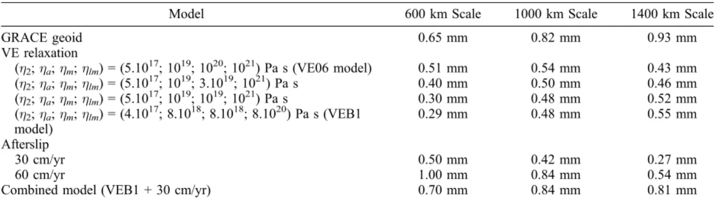
vis-cosity allows us to derive correct geoid amplitudes at all spatial scales. We note that our final model, represented in Figure 9, still slightly lacks energy at the largest scales, and has a bit too much signal at the smallest scales as compared to the data. This excess of signal at the smallest scales may be related to the damping of the GRGS geoids for all From June 2005 to September 2007 From Different Modelsa
Model 600 km Scale 1000 km Scale 1400 km Scale
GRACE geoid 0.65 mm 0.82 mm 0.93 mm VE relaxation (h2;ha;hm;hlm) = (5.10 17 ; 1019; 1020; 1021) Pa s (VE06 model) 0.51 mm 0.54 mm 0.43 mm (h2;ha;hm;hlm) = (5.1017; 1019; 3.1019; 1021) Pa s 0.40 mm 0.50 mm 0.46 mm (h2;ha;hm;hlm) = (5.1017; 1019; 1019; 1021) Pa s 0.30 mm 0.48 mm 0.52 mm (h2;ha;hm;hlm) = (4.1017; 8.1018; 8.1018; 8.1020) Pa s (VEB1 model) 0.29 mm 0.48 mm 0.55 mm Afterslip 30 cm/yr 0.50 mm 0.42 mm 0.27 mm 60 cm/yr 1.00 mm 0.84 mm 0.54 mm
Combined model (VEB1 + 30 cm/yr) 0.70 mm 0.84 mm 0.81 mm
a
For the viscoelastic relaxation,h2is the transient asthenospheric viscosity;hais the steady state asthenospheric viscosity; andhmandhlmare the
220–670 km depth and lower mantle Maxwell viscosity, respectively. The ratios ha/h2= 20 andhlm/ha= 100 are assumed.
Figure 7. CWT at (left) 600 km, (middle) 1000 km, and (right) 1400 km scales of the difference in geoid variation up to spherical harmonic degree 50 between relaxation models having different viscosities in the 220–670 km depth range: effect of lowering the viscosity from 1020 Pa s to 1019 Pa s. The stacking period is from April 2005 to September 2007.
spherical harmonic degree above 30, which may have an impact on our 600 km scale component, whereas the 1000 km and 1400 km scales are more reliable. Results at the larger scales suggest that even lower mantle viscosities might be possible; they might also be related with a nonlinear response of the upper mantle below the astheno-sphere as we discuss below.
[26] From this analysis, we believe that the most
realistic model to fit both the GRACE and the GPS data is obtained when combining a small amount of afterslip at depth (75 cm of slip over the studied period) with viscoelastic relaxation of the upper mantle involving essentially no contrast in steady state viscosity between the asthenosphere and the
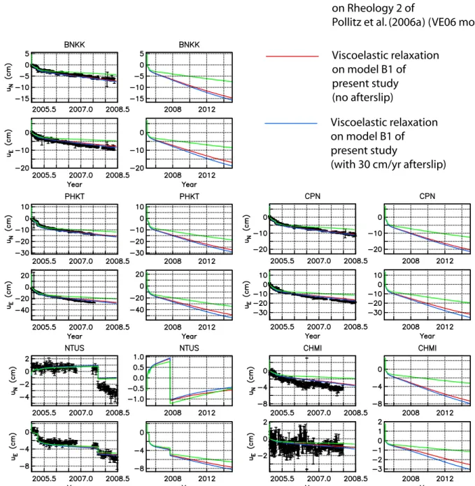
deeper upper mantle. Table 1 summarizes the amount of signal at each scale obtained from each separate model and from the combined model. It clearly shows that afterslip and viscoelastic relax-ation contribute at small scales and at large scales, respectively, thus their balanced combination pro-duces a fit to the GRACE data at all scales. Figure 10 shows the GPS displacements predicted from this combined model, as well as from a model of vis-coelastic relaxation alone using either the VE06 viscosity structure (Table 1) or the modified VEB1 model of the present study (Table 1). Figure 6 illustrates the minimum in GPS data misfit using model VEB1. All time series in Figure 10 are better fitted with the modified viscosity structure (i.e., red
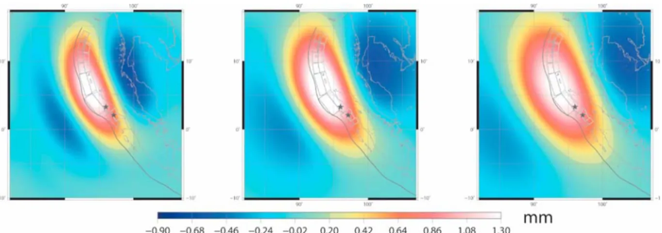
Figure 9. CWT at (left) 600 km, (middle) 1000 km, and (right) 1400 km scales of the geoid variations associated with 75 cm of thrust slip along the fault planes defined by Banerjee et al. [2007] from April 2005 to September 2007, added to the modified relaxation model VEB1 of our study. The coseismic and afterslip fault planes are represented in gray.
Figure 8. CWT at (left) 600 km, (middle) 1000 km, and (right) 1400 km scales of the geoid variations associated with 75 cm of thrust slip along the deeper fault planes defined by Banerjee et al. [2007] with an extended 100 km width from April 2005 to September 2007. The afterslip fault planes are represented in gray.
versus green curves). The addition of afterslip results in only minor differences at most GPS sites (i.e., blue versus green curves in Figure 10) but produces even better agreement with observed time series. The fit to the GPS measurements is good, and remaining misfit is of the same order as the error in interseismic relative velocities (Apel et al., submitted manuscript, 2010) used to correct the original GPS time series. The solid profile in
Figure 11 shows this preferred depth‐dependent viscosity model (east Indian Ocean: GRACE/GPS).
5. Discussion
[27] As a first approximation, we provided here a
simple model to account for the postseismic deformations of the Sumatra‐Andaman 2004 earthquake, but the real rheology of this region is
Figure 10. Horizontal north and east crustal displacements predicted from the different postseismic deformation models, up to year 2008.5 and up to year 2015, compared with the GPS measurements. Model time series include the effect of coseismic offsets from the 2005 Nias earthquake [Banerjee et al., 2007] and 2007 Sumatra earth-quakes [Konca et al., 2008].
certainly more complex. Low‐viscosity areas are indeed expected in the mantle wedge, where the water released by the subducting slab partly melts the mantle rocks [Hirth and Kohlstedt, 2003]. Pollitz et al. [2008] studied the effects of the lateral viscosity variations due to the structure of the subducting slab and to the weaker mantle wedge in the back‐arc region. They concluded that intro-ducing such lateral heterogeneity in the visco-elastic model reduces the amplitude of the Sumatra‐Andaman 2004 postseismic deformation. This can be compensated by increasing the amount of afterslip at the depth. However, geodetic data alone do not allow to precisely quantify the com-peting effects of the viscosity profile and its lateral variations, the slab structure and the afterslip at depth. This is the reason why we preferred to use a simpler model as a first approach. The main information that GRACE and GPS data provide, in any case, is that a low‐viscosity upper mantle is required to adequately fit both data sets.
[28] The viscosity values of our model are
consis-tent with other estimates from the literature. Studies of tilting of continental margins and oceanic islands in response to sea level changes [Nakada and
ment in southeast Iceland [Fleming et al., 2007] indicate the presence of a low‐viscosity zone (LVZ) in the shallow mantle with an effective viscosity much lower than that of the deeper mantle. Moreover, Fleming et al. [2007] constrain the depth range and absolute viscosity in the LVZ to be roughly 30–400 km and 2.1018 Pa s, respectively. This LVZ thus corresponds to the asthenosphere and a part of the underlying upper mantle in our model. Although the tectonic setting in Iceland is different from the Sumatra subduction one, their results indicate the possibility of very low viscosities in the upper mantle. In both cases, the presence of water in the oceanic mantle may also reduce the viscosity [Ranalli, 1995; Bürgmann and Dresen, 2008]. Figure 10 shows the VATNA‐3 model of Fleming et al. [2007] together with our inferred viscosity structure for the eastern Indian Ocean. If these viscosity structures are comparable, then our results of postearthquake relaxation sug-gest that the effective viscosity in the LVZ that describes the response to other loads (glacio‐ isostatic adjustment or sea level changes) represents a combination of the transient and steady state viscosities of the LVZ. Although the magnitude of mantle viscosity is larger beneath an ancient con-tinental region, inferences of a LVZ based on the above studies are consistent with the trade‐off between LVZ thickness and viscosity contrast derived by Paulson and Richards [2009] in a study of postglacial rebound from Hudson Bay. They indeed showed that the observed viscous deforma-tions may be explained by lower viscosities in a thinner LVZ, or larger viscosities in a thicker LVZ.
[29] Transient rheologies have also been suggested
by other geodetic studies of postseismic deforma-tion at time scales of a few days to decades [e.g., Pollitz et al., 2001; Pollitz, 2003], and related to the presence of weak inclusions, transient creep or nonlinear flow in the crust and mantle. For instance, Pollitz et al. [1998] inferred a steady state viscosity of 5 · 1017 Pa s for the oceanic astheno-sphere. This is in agreement with the value of the transient asthenospheric viscosity in the present model, and indicates again the existence of a LVZ in the shallow mantle. Other studies in tec-tonically active continental regions (summarized by Hammond et al. [2009], Bürgmann and Dresen [2008], and Thatcher and Pollitz [2008]) yield similar estimates of the steady state viscosity in the upper mantle, and they are generally much lower than those derived from postglacial rebound stud-ies. However, previous postearthquake studies
Figure 11. Estimates of depth‐dependent mantle vis-cosity derived in oceanic settings. Steady state visvis-cosity is indicated for three different models: long dashed lines indicate southeast Iceland from Fleming et al. [2007, Figure 6b], solid lines indicate east Indian Ocean (GPS) from Pollitz et al. [2006a], and short dashed lines indi-cate east Indian Ocean (GRACE/GPS) from the present study. Note that the lithosphere thickness given by Fleming et al. [2007] is 20 km. The transient viscosity for the east Indian Ocean is labeled with h2.
100 km. The viscosity of 8 · 1018 Pa s inferred for the 220–670 km range in the present study suggests that low steady state viscosity inferred for the shallow mantle persists to much greater depth, well below the base of the asthenosphere, at least below the eastern Indian Ocean.
[30] Such a low viscosity in the 220–670 km depth
range could also be related with a possible non-linear response of the deeper upper mantle to the large stress release of the Sumatra‐Andaman 2004 earthquake. Laboratory experiments show that a nonlinear response of ductile olivine to the stress applied may be expected in a wide range of fre-quencies [Minster and Anderson, 1981]. Linear deformation of olivine in the diffusion creep regime is expected in the lower upper mantle [Karato and Wu, 1993], but these authors also mention that the power law rheology may dominate in upper mantle regions where the stress level is high. In the case of the Sumatra‐Andaman 2004 earthquake, coral morphology and geodetic data show that the Sumatra subduction zone is highly locked [Simoes et al., 2004], and the area around the epicenter of the earthquake had not ruptured historically. At the regional level, the India/Eurasia collision produces very high stresses in the oceanic lithosphere [Deplus, 2001]. Consequently, large amounts of strains and hence stresses have accu-mulated and have been released by the earthquake [Nalbant et al., 2005; Pollitz et al., 2006b]. In this context, a nonlinear rheology is plausible. It would lead to a highly spatially and temporally dependent viscosity, and explain why the effective viscosities inferred from studies of different events may differ by orders of magnitude. Here, nonlinearity may thus account for our low upper mantle viscosity. Such rheology was proposed, at shallower depths, to account for the postseismic deformations of the Denali 2002 Alaska earthquake [Freed et al., 2006] and of the 1992 Landers and 1999 Hector Mine earthquakes [Freed and Bürgmann, 2004]. The magnitude of these earthquakes is between 7.1 and 7.9. In this hypothesis, the low‐viscosity Kelvin element of the Burgers body model approximates the nonlinear behavior of the asthenosphere [Pollitz, 2003]. It could be one of several elements that build a more complex model with time‐varying viscosity. In a similar fashion, our low viscosity in the deeper upper mantle may be a component of a more complex, nonlinear rheology model in response to the large stress released by the Suma-tra‐Andaman 2004 earthquake, the upper mantle viscosity slowly increasing to a higher steady state
1400 km scale we observe in the GRACE data, as compared to our final model, could be due to an imperfect approximation of such nonlinear effects. This hypothesis will have to be confirmed by studies of the GRACE data over longer time scales in the future. As they are very precise at the wave-lengths of mantle relaxation, these data provide an unprecedented view into such possible viscous behavior of the whole upper mantle.
6. Conclusion
[31] From a multiscale analysis of the GRACE
geoids until September 2007, we have isolated the gravity signature of the postseismic signal of the Sumatra‐Andaman Mw = 9.2 2004 earthquake.
The fast growth of geoid variations around the trench during the years following the earthquake cannot be fully explained by the previous viscoelas-tic relaxation models proposed for this earthquake from an analysis of GPS measurements of crustal deformation alone. The GRACE data are particu-larly sensitive to the large‐scale deformation and suggest more deformation at depth than previously modeled. Such observation cannot be accounted for by pure afterslip, which is a smaller‐scale process. It is well explained by a viscoelastic relaxation model with a low upper mantle viscosity, to which afterslip at the downdip continuation of the rup-tured surface is added. In this model, the astheno-sphere (60–220 km depth) has a Burgers body rheology with transient and steady state viscosities equal to 4 · 1017Pa s and 8 · 1018Pa s, respectively, and the mantle below depth 220 km has a Maxwell rheology with viscosity 8 · 1018Pa s for the upper mantle and 8 · 1020Pa s for the lower mantle. Such a hybrid model is also in good agreement with the horizontal GPS displacements in the area. The amplitude of the upper mantle viscosity suggested by this study is within the range of estimates from other regions. The low viscosity ≈1019 inferred for the entire upper mantle may illustrate the nonlinear response of the upper mantle to the large stress release of the Sumatra earthquakes. This will have to be confirmed by further investigations of the GRACE data over longer time spans.
[32] Finally, these results also show the
comple-mentarity between satellite gravity and surface geodetic data and the prospects of their joint analysis. The GRACE data are more sensitive to the effect of the vertical displacements, which is the least precise of the three components of crustal displacement measured by GPS, and fully captures
the deeper layers. Thus, for great subduction zone earthquakes, GRACE detects well the density var-iations resulting from large‐scale deformation and provides a unique view of the mantle viscous response to the earthquake. In contrast, the surface GPS data are more sensitive to the horizontal dis-placements and to relatively shallow mantle vis-cosity structure. Thus, jointly modeling those two data sets leads to a better view of the geodynamic processes. This shows the broad interest in satellite gravity data, especially for subduction earthquakes studies where the surface network may be sparse.
Acknowledgments
[33] We are very grateful to Roland Bürgmann for helping us to improve our manuscript. Isabelle Panet was partly supported by a CNES postdoctoral fellowship, and this work was sup-ported by CNES through the TOSCA committee. Valentin Mikhailov was supported by grants 09‐05‐00258 and 09‐ 05‐91056 of the Russian Foundation for Basic Research. We thank the Associate Editor, Thorsten Becker, and two anony-mous reviewers for their constructive comments that improved our manuscript. Maps in Figures 1, 2, 4, and 6–9 were plotted using the GMT software [Wessel and Smith, 1995]. This is IPGP contribution 2654.
References
Altamimi, Z., P. Sillard, and C. Boucher (2002), ITRF2000: A new release of the International Terrestrial Reference Frame for earth science applications, J. Geophys. Res., 107(B10), 2214, doi:10.1029/2001JB000561.
Ammon, C., et al. (2005), Rupture process of the 2004 Sumatra‐ Andaman earthquake, Science, 308, 1133–1139.
Banerjee, P., F. Pollitz, and R. Bürgmann (2005), Size and duration of the great 2004 Sumatra‐Andaman earthquake from far‐field static offsets, Science, 308, 1769–1772. Banerjee, P., F. Pollitz, B. Nagarajan, and R. Burgmann
(2007), Co‐seismic slip distributions of the 26 December 2004 Sumatra‐Andaman and 28 March 2005 Nias earth-quakes from GPS static offsets, Bull. Seismol. Soc. Am., 97 (1A), S86–S102.
Biancale, R., J.‐M. Lemoine, G. Balmino, S. Loyer, S. Bruinsma, F. Perosanz, J.‐C. Marty, and P. Gegout (2007), Five years of decadal geoid variations from GRACE and LAGEOS data [CD‐ROM], Groupe de Rech. de Geod. Spatiale, Cent. Natl. d’Etudes Spatiales, Toulouse, France.
Bürgmann, R., and G. Dresen (2008), Rheology of the lower crust and upper mantle: Evidence from rock mechanics, geod-esy and field observations, Annu. Rev. Earth Planet. Sci., 36, 531–567, doi:10.1146/annurev.earth.36.031207.124326. Cannelli, V., D. Melini, A. Piersanti, and E. Boschi (2008),
Postseismic signature of the 2004 Sumatra earthquake on low‐degree gravity harmonics, J. Geophys. Res., 113, B12414, doi:10.1029/2007JB005296.
great M‐w 9.15 Sumatra‐Andaman earthquake of 2004, Bull. Seismol. Soc. Am., 97, S152–S173.
Curray, J. (2005), Tectonics and history of the Andaman Sea region, J. Asian Earth Sci., 25, 187–232.
de Linage, C., L. Rivera, J. Hinderer, J.‐P. Boy, Y. Rogister, S. Lambotte, and R. Biancale (2008), Separation of coseismic and postseismic gravity changes for the 2004 Sumatra‐ Andaman earthquake from 4.6 yr of GRACE observations and modelling of the coseismic change by normal‐modes summation, Geophys. J. Int., 176(3), 695–714.
Deplus, C. (2001), Indian Ocean actively deforms, Science, 292(5523), 1850–1851.
Deplus, C., M. Diament, H. Hébert, G. Bertrand, S. Dominguez, J. Dubois, J. Malod, B. Pontoise, and J.‐J. Sibilla (1998), Direct evidence of active deformation in the eastern Indian oceanic plate, Geology, 26(2), 131–134.
de Viron, O., I. Panet, V. Mikhailov, M. Van Camp, and M. Diament (2008), Retrieving earthquake signature in GRACE gravity solutions, Geophys. J. Int., 174(1), 14–20. Diament, M., H. Harjono, K. Karta, C. Deplus, D. Dahrin,
M. T. Zen, M. Grard, O. Lassal, A. Martin, and J. Malod (1992), The Mentawai Fault Zone off Sumatra, a new key for the geodynamics of Western Indonesia, Geology, 20, 259–262.
Dickey, J., et al. (1997), Satellite Gravity and the Geosphere, Natl. Acad. Press, Washington, D. C.
Dziewonski, A. M., and D. L. Anderson (1981), Preliminary Reference Earth Model (PREM), Phys. Earth Planet. Inter., 25, 297–356.
Fleming, K., Z. Martinec, and D. Wolf (2007), Glacial‐isostatic adjustment and the viscosity structure underlying the Vatnajokull Ice Cap, Iceland, Pure Appl. Geophys., 164, 751–768. Freed, A. M., and R. Bürgmann (2004), Evidence of power‐
law flow in the Mojave desert mantle, Nature, 430, 548–551. Freed, A. M., R. Bürgmann, E. Calais, and J. T. Freymueller (2006), Stress‐dependent power‐law flow in the upper man-tle following the 2002 Denali, Alaska, earthquake, Earth Planet. Sci. Lett., 252, 481–489.
Gross, R., and B. Chao (2001), The gravitational signature of earthquakes, in Gravity, Geoid and Geodynamics 2000, Int. Assoc. of Geod. Symp., vol. 123, pp. 205–210, Springer, New York.
Gudmundsson, O., and M. Sambridge (1998), A regionalized upper mantle (RUM) seismic model, J. Geophys. Res., 103, 7121–7136.
Hager, B. H. (1991), Mantle viscosity—A comparison of models from postglacial rebound and from the geoid, plate driving forces, and advected heat flux, in Glacial Isostasy, Sea Level and Mantle Rheology, pp. 493–513, Kluwer Acad., Dordrecht, Netherlands.
Hammond, W. C., C. Kreemer, and G. Blewitt (2009), Geodetic constraints on contemporary deformation in the Northern Walker Lane: 3. Central Nevada seismic belt postseismic relaxation, in Late Cenozoic Structure and Evolution of the Great Basin, Sierra Nevada Transition, Spec. Pap. Geol. Soc. Am., 447, 33–54, doi:10.1130/2009.2447(03).
Han, S.‐C., and F. Simons (2008), Spatiospectral localization of global geopotential fields from the Gravity Recovery and Climate Experiment (GRACE) reveals the coseismic gravity change owing to the 2004 Sumatra‐Andaman earthquake, J. Geophys. Res., 113, B01405, doi:10.1029/2007JB004927. Han, S.‐C., C. K. Shum, M. Bevis, C. Ji, and C.‐Y. Kuo (2006), Crustal dilatation observed by GRACE after the 2004 Sumatra‐Andaman earthquake, Science, 313, 658–662.
(2008), Implications of postseismic gravity change following the great 2004 Sumatra‐Andaman earthquake from the regional harmonic analysis of GRACE intersatellite tracking data, J. Geophys. Res., 113, B11413, doi:10.1029/ 2008JB005705.
Hashimoto, M., N. Chhoosakul, M. Hashizume, S. Takemoto, H. Takiguchi, Y. Fukada, and K. Fujimori (2006), Crustal deformations associated with the Great Sumatra‐Andaman earthquake deduced from continuous GPS observations, Earth Planets Space, 58, 127–139.
Herring, T., R. King, and S. McClusky (2008a), GLOBK: Global Kalman filter VLBI and GPS analysis program, release 10.3, Mass. Inst. of Technol., Cambridge, Mass. Herring, T., R. King, and S. McClusky (2008b),
Documenta-tion for the GAMIT GPS analysis software, release 10.3, Mass. Inst. of Technol., Cambridge, Mass.
Hirth, G., and D. Kohlstedt (2003), Rheology of the upper mantle and the mantle wedge: A view from the experimental-ists, in Inside the Subduction Factory, Geophys. Monogr. Ser., vol. 138, edited by J. Eiler, pp. 83–105, AGU, Washington, D. C.
Holschneider, M. (1995), Wavelets: An Analysis Tool, Oxford Sci., Oxford, U. K.
Holschneider, M., A. Chambodut, and M. Mandea (2003), From global to regional analysis of the magnetic field on the sphere using wavelet frames, Phys. Earth Planet. Inter., 135, 107–124.
Karato, S., and P. Wu (1993), Rheology of the upper mantle: A synthesis, Science, 260, 771–778.
King, S. D. (1995), The viscosity structure of the mantle, U.S. Natl. Rep. Int. Union Geod. Geophys. 1991–1994, Rev. Geophys., 33, 11–18.
Konca, A. O., et al. (2008), Partial rupture of a locked patch of the Sumatra megathrust during the 2007 earthquake sequence, Nature, 456, 631–635.
Lay, T., et al. (2005), The great Sumatra‐Andaman earthquake of 26 December 2004, Science, 308, 1127–1133.
Lemoine, J.‐M., S. Bruinsma, S. Loyer, R. Biancale, J.‐C. Marty, F. Perosanz, and G. Balmino (2007), Temporal grav-ity field models inferred from GRACE data, Adv. Space Res., 39, 1620–1629.
Masterlark, T., C. DeMets, H. Wang, O. Sanchez, and J. Stock (2001), Homogeneous versus heterogeneous subduction zone models: Coseismic and post‐seismic deformation, Geo-phys. Res. Lett., 28, 4047–4050.
Mikhailov, V., S. Tikhostky, M. Diament, I. Panet, and V. Ballu (2004), Can tectonic processes be recovered from new satel-lite gravity data?, Earth Planet. Sci. Lett., 228 (3/4), 281–297. Minster, J. B., and D. L. Anderson (1981), A model of dislo-cation‐controlled rheology for the mantle, Philos. Trans. R. Soc. London, 299, 319–356.
Nakada, M., and K. Lambeck (1987), Glacial rebound and rel-ative sea level variations: A new appraisal, Geophys. J. R. Astron. Soc., 90, 171–224.
Nakada, M., and K. Lambeck (1989), Late Pleistocene and Holocene sea‐level change in the Australian region and man-tle rhology, Geophys. J. Int., 96, 497–517.
Nalbant, S. S., S. Steacy, K. Sieh, D. Natawidjaja, and J. McCloskey (2005), Earthquake risk on the Sunda trench, Nature, 435, 756–757.
Ogawa, R., and K. Heki (2007), Slow post‐seismic recovery of geoid depression formed by the 2004 Sumatra‐Andaman earthquake by mantle water diffusion, Geophys. Res. Lett., 34, L06313, doi:10.1029/2007GL029340.
O. Jamet (2006), New insights on intra‐plate volcanism in French Polynesia from wavelet analysis of GRACE, CHAMP and sea‐surface data, J. Geophys. Res., 111, B09403, doi:10.1029/2005JB004141.
Panet, I., V. Mikhailov, M. Diament, F. Pollitz, G. King, O. de Viron, M. Holschneider, R. Biancale, and J. M. Lemoine (2007), Co‐seismic and post‐seismic signatures of the Sumatra December 2004 and March 2005 earthquakes in GRACE satellite gravity, Geophys. J. Int., 171(1), 177– 190, doi:10.1111/j.1365-246X.2007.03525.x.
Paul, J., A. R. Lowry, R. Bilham, S. Sen, and R. Smalley Jr. (2007), Postseismic deformation of the Andaman Islands fol-lowing the 26 December, 2004 Great Sumatra‐Andaman earthquake, Geophys. Res. Lett., 34, L19309, doi:10.1029/ 2007GL031024.
Paulson, A., and M. A. Richards (2009), On the resolution of radial viscosity structure in modeling long‐wavelength post‐ glacial rebound data, Geophys. J. Int., 179, 1516–1526, doi:10.1111/j.1365-246X.2009.04362.x.
Pollitz, F. (1996), Co‐seismic deformation from earthquake faulting on a layered spherical Earth, Geophys. J. Int., 125, 1–14.
Pollitz, F. (1997), Gravitational‐viscoelestic postseismic relax-ation on a layered spherical Earth, J. Geophys. Res., 102, 17,921–17,941.
Pollitz, F. (2003), Transient rheology of the uppermost mantle beneath the Mojave Desert, California, Earth Planet. Sci. Lett., 215, 89–104.
Pollitz, F., R. Bürgmann, and B. Romanowicz (1998), Viscos-ity of oceanic asthenosphere inferred from remote triggering of earthquakes, Science, 280, 1245–1249.
Pollitz, F., C. Wicks, and W. Thatcher (2001), Mantle flow beneath a continental strike‐slip fault: Post‐seismic deforma-tion after the 1999 Hector Mine earthquake, Science, 293, 1814–1818.
Pollitz, F., P. Banerjee, and R. Bürgmann (2006a), Post‐seismic relaxation following the great 2004 Sumatra‐Andaman earth-quake on a compressible self‐gravitating Earth, Geophys. J. Int., 167, 397–420.
Pollitz, F., P. Banerjee, R. Bürgmann, M. Hashimoto, and N. Choosakul (2006b), Stress changes along the Sunda trench following the 26 December 2004 Sumatra‐Andaman and 28 March 2005 Nias earthquakes, Geophys. Res. Lett., 33, L06309, doi:10.1029/2005GL024558.
Pollitz, F., P. Banerjee, K. Grijalva, B. Nagarajan, and R. Bürgmann (2008), Effect of 3D visco‐elastic structure on post‐seismic relaxation from the 2004 M = 9.2 Sumatra earthquake, Geophys. J. Int., 173, 189–204, doi:10.1111/ j.1365-246X.2007.03666.x.
Ranalli, G. (1995), Rheology of the Earth, 413 pp., Chapman and Hall, London.
Ray, R. D., and S. B. Luthcke (2006), Tide model errors and GRACE gravimetry: Towards a more realistic assessment, Geophys. J. Int., 167, 1055–1059.
Schrama, E. J. O., and P. N. A. M. Visser (2007), Accuracy assessment of the monthly GRACE geoids based upon a simulation, J. Geod., 81, 67–80, doi:10.1007/s00190-006-0085-1.
Simoes, M., J.‐P. Avouac, R. Cattin, and P. Henry (2004), The Sumatra subduction zone: A case for a locked fault zone extending into the mantle, J. Geophys. Res., 109, B10402, doi:10.1029/2003JB002958.
Simons, F., J. Hawthorne, and C. Beggan (2009), Efficient analysis and representation of geophysical processes using
Eng., 7446, 74460G, doi:10.1117/12.825730.
Sun, W., and S. Okubo (2004), Coseismic deformations detect-able by satellite gravity missions: A case study of Alaska (1964, 2002) and Hokkaido (2003) earthquakes in the spec-tral domain, J. Geophys. Res., 109, B04405, doi:10.1029/ 2003JB002554.
Thatcher, W., and F. Pollitz (2008), Temporal evolution of con-tinental lithospheric strength in actively deforming regions, GSA Today, 18(4–5), 4–11, doi:10.1130/GSAT01804-5A.1.
Andaman earthquake from GPS measurements in southeast Asia, Nature, 436, 201–206.
Wahr, J., M. Molenaar, and F. Bryan (1998), Time variability of the Earth’s gravity field: Hydrological and oceanic effects and their possible detection using GRACE, J. Geophys. Res., 103, 30,205–30,229.
Wessel, P., and W. H. F. Smith (1995), New version of the Generic Mapping Tool released, Eos Trans. AGU, 76, 329.