HAL Id: hal-00295530
https://hal.archives-ouvertes.fr/hal-00295530
Submitted on 16 Sep 2004
HAL is a multi-disciplinary open access
archive for the deposit and dissemination of
sci-entific research documents, whether they are
pub-lished or not. The documents may come from
teaching and research institutions in France or
abroad, or from public or private research centers.
L’archive ouverte pluridisciplinaire HAL, est
destinée au dépôt et à la diffusion de documents
scientifiques de niveau recherche, publiés ou non,
émanant des établissements d’enseignement et de
recherche français ou étrangers, des laboratoires
publics ou privés.
differences in TOMCAT model performance
N. H. Savage, Kathy S. Law, J. A. Pyle, A. Richter, H. Nüß, J. P. Burrows
To cite this version:
N. H. Savage, Kathy S. Law, J. A. Pyle, A. Richter, H. Nüß, et al.. Using GOME NO2 satellite data to
examine regional differences in TOMCAT model performance. Atmospheric Chemistry and Physics,
European Geosciences Union, 2004, 4 (7), pp.1895-1912. �hal-00295530�
www.atmos-chem-phys.org/acp/4/1895/
SRef-ID: 1680-7324/acp/2004-4-1895
Chemistry
and Physics
Using GOME NO
2
satellite data to examine regional differences in
TOMCAT model performance
N. H. Savage1, K. S. Law1,*, J. A. Pyle1, A. Richter2, H. N ¨uß2, and J. P. Burrows2
1Centre for Atmospheric Science, Chemistry Department, University of Cambridge, UK
2Institute of Environmental Physics, University of Bremen, NW1, Kufsteiner Strasse 1, D-28359 Bremen, Germany *Now at: Service d’Aeronomie, CNRS/IPSL, Paris, France
Received: 26 February 2004 – Published in Atmos. Chem. Phys. Discuss.: 12 May 2004 Revised: 13 September 2004 – Accepted: 14 September 2004 – Published: 16 September 2004
Abstract. This paper compares column measurements of
NO2made by the GOME instrument on ERS-2 to model
re-sults from the TOMCAT global CTM. The overall correlation between the model and observations is good (0.79 for the whole world, and 0.89 for North America) but the modelled columns are larger than GOME over polluted areas (gradient of 1.4 for North America and 1.9 for Europe). NO2columns
in the region of outflow from North America into the Atlantic are higher in winter in the model compared to the GOME re-sults, whereas the modelled columns are smaller off the coast of Africa where there appear to be biomass burning plumes in the satellite data. Several hypotheses are presented to explain these discrepancies. Weaknesses in the model treatment of vertical mixing and chemistry appear to be the most likely explanations.
1 Introduction
Nitrogen dioxide (NO2) plays a central role in tropospheric
chemistry. NO2photolysis is the major tropospheric source
of ozone; NO2 is recycled in a catalytic manner via
reac-tions with peroxy radicals (Haagen-Smit, 1952). In many regions of the atmosphere ozone production is NOx-limited
(e.g. Chameides et al., 1992). Therefore a correct simula-tion of the budget of NOx(NO2+NO) is a prerequisite for an
accurate model ozone budget. The Intergovernmental Panel on Climate Change Third Assessment Report (IPCC-TAR, Houghton et al., 2001) gives an estimate of a global average radiative forcing of +0.35±0.15 W m−2due to increases in
tropospheric ozone since pre-industrial times making it the third most important greenhouse gas after CO2 and CH4.
They also assigned this forcing a medium level of scientific understanding and highlighted how model-model differences Correspondence to: N. H. Savage
affected calculated ozone budgets. Understanding the contri-bution of NOxis clearly essential. In addition to its role in the
ozone budget, nitrogen dioxide is also oxidised to form nitric acid which plays an important role in acidification and can also act as a nutrient with important impacts on ecosystems (e.g. Borrell et al., 1997).
Model validation studies using a variety of data sets have shown that models find the simulation of the NOy budget
to be a challenge. For example Grewe et al. (2001) found that two coupled chemistry climate models were unable to reproduce the gradient in NOx mixing ratio between North
America and the Atlantic Ocean and had problems correctly reproducing vertical gradients. Thakur et al. (1999) found that models tended to under-predict global free tropospheric NO while over-predicting HNO3 and PAN. Brunner et al.
(2003) found that results for NOxdiffered quite significantly
between models. Specific problems included the inability to model locally elevated NOxin plumes. For many field
cam-paigns models under-predicted NOx, especially in regions
re-cently impacted by lightning.
A major part of the challenge in improving model perfor-mance is the large number of different processes which have an impact on chemical concentrations and distributions. If the total emissions of one or more chemical compounds are incorrect, or if these emissions are not distributed correctly across the world, the model will be unable to predict the con-centrations of short lived species accurately. As most emis-sions occur close to the ground, dry deposition and bound-ary layer mixing have a strong impact on the total burden of many species. The model then needs to simulate the large scale advection of the chemical species. Convection and other processes such as frontal uplifting of air masses not only redistribute species vertically but as the wind speeds increase with height have a substantial impact on the hori-zontal distribution. In addition, the lifetime and subsequent chemistry of NOxis also a function of height. Uplifted air
key reservoir of NOx. The photolysis of nitric acid is also
more rapid at higher levels and so is more likely to regener-ate NOx unless it is removed by washout. These and many
other changes in the chemical environment with height, im-ply that the lifetime and distribution of NO2will be strongly
influenced by the speed and extent of vertical transport. The rate of ozone production is also affected due to its non-linear dependence on NOxconcentration (e.g. Sillman et al., 1990).
Finally, in order to correctly model the distribution and concentration of any species, the chemical reactions in which it is involved must be adequately modelled. So, errors in model results for any particular species may be due not to model problems in emissions and physical processes affect-ing the species of interest, but may result from problems in modelling other related compounds. For example, if the modelled concentrations of methane are too high this might reduce OH concentrations thus increasing the lifetime of NOx.
With this degree of interaction and complexity in the at-mospheric chemistry system, the physical and chemical pro-cesses occurring in the atmosphere have to be simplified in models. The broader the range of measurements used to validate models the better. Long term measurements at ground stations have the advantage of giving a long time se-ries but have restricted spatial coverage. Aircraft measure-ments have been invaluable to further our understanding but offer only limited spatial and temporal coverage (see for ex-ample Thakur et al., 1999). Satellite measurements offer the advantage of making measurements which are both global and long term.
Several recent studies have used a combination of GOME satellite measurements with global models to assess both the consistency of the GOME data and validate models. Velders et al. (2001) compared monthly average NO2columns from
the global CTMs IMAGES and MOZART to GOME mea-surements for 1997. They found that the columns over Eu-rope and North America were of the same order as those calculated by the MOZART model but were a factor of 2– 3 higher over Asia. Lauer et al. (2002) compared a clima-tological data set for NO2to the first 5 years of the GOME
measurements. They examined the seasonal evolution of the column over Europe, the Eastern USA, Africa, South Amer-ica, Australia and Southeast Asia. They found an overestima-tion by the GCM of 2 to 3 times. Kunhikrishnan et al. (2004) compared the results of the MATCH-MPIC model from 1997 and 1998, with a focus on the seasonal columns over various parts of the Asian region. They found that seasonal average NO2columns from the model were comparable to the
satel-lite results but there were problems with the seasonal cycle over India. Martin et al. (2002) calculated correlation coef-ficients between GOME and GEOS-CHEM calculations for the USA and the whole world using data from July 1996. For the USA the GOME results were within 18% of the model results and had a correlation coefficient of 0.78.
In this paper the previous analyses are extended by bining the methods of correlation studies and the use of com-parisons of seasonal columns, using a wider range of regions and examining an entire year’s output from a CTM. The re-sults are compared to those of previous studies. We aim to show how GOME NO2column measurements can be used to
highlight areas of disagreement as a means to target and test future model development and develop validation strategies. This must still however be considered a preliminary attempt at using tropospheric satellite data in connection with model results. Identifying areas of disagreement between the model and satellite measurements can give insight into which model processes require development as well as identifying regions of the world where especially important and/or interesting events are taking place and should be studied in more detail. This will further our understanding of the atmospheric chem-istry system as a whole. However this is an emerging area of research and much work remains to be done before the satel-lite observations can be exploited to their full potential.
Section 2 discusses how NO2 columns were retrieved
from the GOME data and Sect. 3 describes TOMCAT, the chemistry-transport model used for this study. The model results are compared to the GOME retrievals in Sect. 4 and reasons for differences are examined in Sect. 5.
2 Satellite data
2.1 Instrument Description
GOME is a spectrometer on board ERS-2. It was launched on 20 April 1995 and flies in a sun-synchronous, polar or-bit at an average height of 785 km above the Earth’s sur-face (Burrows et al., 1999, and references therein). The GOME instrument observes in nadir viewing geometry the light (UV/visible) scattered back from the atmosphere and reflected at the ground. Once per day, it also observes the ex-traterrestrial solar irradiance. The instrument is designed to observe simultaneously the spectral range between 232 and 793 nm. The atmosphere is scanned with a spatial resolu-tion of 320 km×40 km (across track×along track) (forward scan) and 960 km×40 km (back scan). Each individual orbit of ERS-2 takes about 100 min. Although the repeating cycle of an orbit is 35 days, nearly global coverage (except for a small gap around the poles) is achieved within three days ap-plying the maximum scan width of 960 km (ESA, 1995). As a result of the sun-synchronous orbit, the measurements in low and middle latitudes are always taken at the same local time (LT) with, for example, the northern mid-latitudes being crossed at about 10:45 LT.
2.2 NO2column retrieval
The trace gas retrieval of NO2is achieved using the DOAS
technique (Differential Optical Absorption Spectroscopy). This technique utilises the atmospheric absorption, defined
as the natural logarithm of the ratio of the extraterrestrial ir-radiance and the earth-shine ir-radiance, for a selected spectral window. This is compared with reference absorption spec-tra of gases absorbing in the specspec-tral window and a polyno-mial of low order. The polynopolyno-mial describes the scattering and broad absorption in the window. The slant column of a gas is derived from the differential absorption of the gas in question and to a first approximation is the integrated con-centration along the light paths through the atmosphere. For this study, the spectral window from 425 to 450 nm has been used, the spectra of NO2, O3, O4and H2O and a reference
Ring spectrum being fitted (Richter and Burrows, 2002). The resultant slant columns of NO2 include both the
stratospheric and the tropospheric signal. To isolate the tropospheric column, a modified reference sector or tropo-spheric excess method (TEM) was applied. Originally, in this method measurements taken over the Pacific Ocean were subtracted from all other measurements assuming that this region has negligible tropospheric NO2columns and that the
stratosphere is zonally invariant with respect to NO2(Richter
and Burrows, 2002). Here, the stratospheric zonal variabil-ity was explicitly taken into account by using daily strato-spheric NO2fields from the 3D-CTM SLIMCAT
(Chipper-field, 1999) sampled at the time of GOME overpass. To ac-count for differences between the stratospheric columns as measured by GOME and those modelled by SLIMCAT, the model results were normalised to the values in the reference sector. With this correction, the consistency of the GOME NO2columns was much improved in particular at Northern
mid and high latitudes in spring. It has to be pointed out that as a result of the normalisation the values still repre-sent a tropospheric excess which does not account for the residual tropospheric NO2 column in the reference region.
The changes in retrieved columns introduced by using this revised method are usually small in polluted regions (of the order of 10%) but can be very large (100%) in those cases, where the TEM fails, for example in higher latitudes (>55 degrees) during vortex excursions. For these situations, the TEM yields alternating regions of large positive and nega-tive values, and using the SLIMCAT fields for the correction brings these numbers much closer to zero as one would ex-pect. Therefore, the absolute instead of the relative differ-ences between the two data products are a better indicator, and these are typically smaller than 1×10¹⁵molec. cm−2in clean regions but can be as large as 4×10¹⁵molec. cm−2in polluted regions. The latter results from the smaller airmass factors in polluted regions that amplify any error made in the stratospheric correction.
The tropospheric slant columns are converted to vertical columns by the application of an air mass factor, AMF. The AMF describes the effective length of the light path through the atmosphere relative to a vertical transect and is derived from radiative transfer calculations. The value of the AMF depends on the viewing geometry and the solar zenith angle, but also on surface albedo, vertical gas profile, clouds and
atmospheric aerosol. In this study, the AMFs used have been improved compared to the ones described in Richter and Bur-rows (2002) in several respects. The value used for surface albedo is taken from the monthly climatology of Koelemei-jer et al. (2001) which is based on GOME measurements; surface elevation is accounted for and extinction by aerosol is treated using three different scenarios (maritime, rural and urban) which were selected based on the geographical lo-cation. Most importantly, the vertical profile of NO2 used
is taken from the daily results of the TOMCAT model run for 1997 described below. For each TOMCAT model grid cell, airmass factors are calculated for a range of solar zenith angles using the model profile and appropriate settings for altitude, aerosol, and surface albedo. For each GOME mea-surement, the airmass factor for the closest model profile was used to convert it to vertical columns. This implies that the comparisons shown are self consistent, in particular for trans-port events where vertical displacement changes the sensitiv-ity of GOME to the NO2. This greatly reduces the
uncer-tainty in the comparison as discussed in Eskes and Boersma (2003). The impact of this on the model-data comparison is discussed later. It is important to note that the airmass factors depend critically on the vertical profile determined by the model. In a recent intercomparison within the Eu-ropean project POET, differences of up to a factor of two were observed for airmass factors based on different mod-els in source regions, indicting that self consistency is cru-cial for model – measurement comparisons, but does not necessarily improve absolute accuracy. Stratospheric NO2
is not included in the airmass factor calculation as the tro-pospheric slant columns have already been corrected for the stratospheric contribution as explained above, and the influ-ence of stratospheric NO2 on the radiative transfer can be
neglected (Richter and Burrows, 2002; Velders et al., 2001). More details of retrieval methods and a full error analysis can be found in Richter and Burrows (2002).
For this study, monthly means of the tropospheric NO2
column amounts (January 1997 to December 1997) have been used. Using a simple intensity threshold algorithm, the data were selected to be cloud free, i.e. only pixels hav-ing a cloud coverage below a threshold value of 10% were used to derive the tropospheric NO2 column amounts from
the GOME measurements. No additional cloud correction was applied, in contrast to other studies (Martin et al., 2002; Boersma et al., 2004).
2.3 GOME retrieval errors
As with all remote sensing measurements, the retrieval of NO2columns from GOME is based on a number of a priori
assumptions that can introduce errors in the final product. The main uncertainties are related to the vertical distribution of the NO2, the impact of aerosols, and clouds.
By using vertical profiles from the TOMCAT model run in the data analysis, the retrieval is self-consistent (but not
necessarily correct) and any such errors introduced by in-correct TOMCAT profiles are properly discussed under the sections on model errors.
Aerosols have been taken into account in the retrieval in a rather general manner, with only 3 different aerosol scenar-ios (maritime, rural and urban). Clearly in regions of intense biomass burning visibility can be much reduced, affecting the data but this is not yet accounted for in the analysis. There-fore, the GOME NO2columns retrieved for such conditions
will tend to underestimate the atmospheric NO2content.
Clouds have been treated by rejecting measurements above a threshold value of roughly 10%, thereby reducing the impact of clouds on the retrieval. However, as discussed in several papers (Velders et al., 2001; Richter and Burrows, 2002; Martin et al., 2002) even relatively small cloud frac-tions can have a significant effect on the result, leading to underestimations of up to 40%, in particular in industrialised regions in winter. Clouds can also lead to an overestimation of NO2 columns if a significant amount of NO2 is located above or within a low cloud layer. There also is the problem of the reduced number of available points in the monthly av-erage in particular in winter in mid-latitudes, and in fact un-der these conditions there often are only a few GOME mea-surements in a 1×1 degree grid box per month, making it less representative of the monthly average.
By applying a cloud screening, there also is a systematic bias in the measurements excluding certain atmospheric situ-ations. For example, transport of pollutants is often linked to frontal systems, which are associated with cloud formation and these will be excluded from the GOME data set. In win-ter the region to the east of Europe is very cloudy and there is little or no GOME data.
A more quantitative but still rough estimate of the uncer-tainties of the GOME NO2retrieval used in this study is to
assume an absolute error of the order of 4×10¹⁴molec. cm−2 and a relative error of the order of 30–50%. This is in line with the recent paper of Boersma et al. (2004) although they discussed a different retrieval algorithm. However, the main error sources are similar in both retrievals, and most conclu-sions in that paper should be valid for this work as well. As discussed by Boersma et al. (2004), the retrieval errors are a function of many parameters, and therefore depend on ge-olocation and season. However, the main driver for the size of the relative error is the absolute NO2 column, and with
the simple approximation given above, very similar error es-timates are derived as those given in Boersma et al. (2004).
3 TOMCAT global model
3.1 TOMCAT model description
TOMCAT is a global three dimensional chemistry-transport model (CTM). Meteorological analyses from the European Centre for Medium Range Weather Forecasting (ECMWF)
are used as input to the model for winds, temperatures and humidity. ECMWF data is read at a frequency of 6 h and the meteorological fields are interpolated in time to each model timestep. Tracer transport is calculated using the Prather advection scheme (Prather, 1986) with a 30 min dynamical time-step. Moist convective transport of tracers is performed using a mass flux scheme (Tiedtke, 1989) and a non-local vertical diffusion scheme is used based on that developed for the NCAR Community Climate Models, Version 2 (Holt-slag and Boville, 1993). This scheme is capable of resolv-ing the diurnal cycle of boundary layer mixresolv-ing and the mod-elled height of the boundary layer shows a seasonal varia-tion in line with observavaria-tions. For more details see Wang et al. (1999). The chemistry is integrated using the ASAD chemistry package (Carver et al., 1997). There is no het-erogeneous loss of N2O5on aerosol in the model at present.
However the reaction of N2O5with gas phase water vapour is
included. The version of the model used here has 31 vertical levels and a horizontal resolution of approximately 2.8×2.8◦ from the ground up to 10 hPa and has a total of 39 chemical species of which 30 are advected. The TOMCAT model was run with a 4 month spin up from September 1996. Model re-sults for the whole of 1997 were used to compare to GOME data.
The emissions data set used here is the same as that used for the POET model intercomparison study (Savage et al., 2003). The anthropogenic emissions are based on Edgar 3 (Olivier et al., 2001) modified to be appropriate for 1997 as described in Olivier et al. (2003). Biomass burning emissions however are based on climatological values and so are not specific to 1997. This is particularly significant as 1997 saw unusual biomass burning emissions due to the effect of the strong El Ni˜no in that year. However as can be seen from Figs. 1 to 4 the emission inventory used in TOMCAT for this experiment is in good agreement with the ATSR firecount data over Africa. The main region where the emissions used for this run did not agree well with the inventory is the area around Indonesia. It can also be seen that especially over the Pacific there are big interannual variations in intensity and location fires. The conclusions here are based on 1997 which is an usual year for biomass burning, however this is less of an issue for Africa which is focused on in this study.
For more details of the model intercomparison see Savage et al. (2003). All surface and aircraft emissions are based on monthly mean data but are interpolated to give a smooth variation in emissions from day to day. Lightning emissions are calculated from the model convection scheme based on the parameterisation of Price and Rind (1992) and are scaled to a global annual total of 5 Tg(N) per year.
3.2 Radon tracer experiment
Radon is a chemically inert tracer which undergoes radioac-tive decay with a lifetime of 5.5 days. Its major emission sources are over land and it has been used previously in
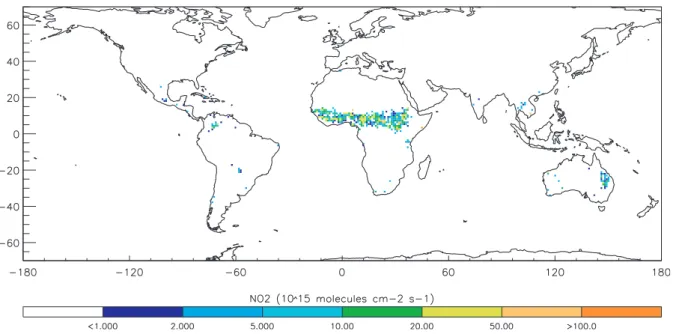
Fig. 1. Model monthly mean biomass burning NOxemissions for January 1997.
model intercomparison studies to examine model transport properties (see for example Jacob et al., 1997; Rasch et al., 2000). As part of the POET intercomparison study (Savage et al., 2003) the TOMCAT model performed the radon ex-periment described in Jacob et al. (1997) for the year 1997 allowing transport processes in the model to be assessed. The results are useful as a means of separating physical and chemical influences on the NO2distribution.
3.3 Model data processing
In order that the model and satellite data are truly compa-rable some care has been taken in processing the model re-sults. There are two main issues to be addressed. Firstly the ERS-2 satellite is in a sun synchronous orbit and has an equator crossing time of 10:30. Standard TOMCAT model output is at 0:00, 06:00, 12:00 and 18:00 GMT so the local time of output varies as a function of longitude. In order to remove this effect, the model was modified to output data ev-ery time-step for those grid points where the local time was close to 10:30, in addition to producing the standard model output. The second issue concerns the separation of the tro-pospheric and stratospheric columns. Although TOMCAT is a tropospheric model the top levels extend into the strato-sphere and so removal of this component is necessary. To make this as close as possible to the TEM method used for the satellite data, as outlined above, the following procedure was used: first the column up to the 350 K isentropic level (the bottom level of the SLIMCAT data used for tropospheric removal) was calculated and then a clean sector average was subtracted. This is referred to as the “best” method. Due to
Fig. 2. ATSR firecounts for January 1997 (top) and 1998 (bottom).
the subtraction from the model results of this clean sector av-erage there are for some grid cells negative model columns. This is an artifact of applying the same algorithm as used to calculate the GOME columns and does not mean that model has grid point values which are negative.
In order to evaluate the importance of the methods used to determine the modelled tropospheric columns two other
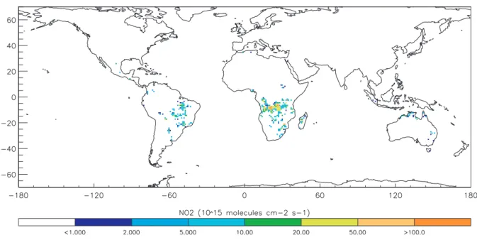
Fig. 3. Model monthly mean biomass burning NOxemissions for July 1997.
Fig. 4. ATSR firecounts for July 1997 (top) and 1998 (bottom).
methods of calculating the column were used. In the first of these a monthly mean of the standard model 6 hourly output files was calculated to give a 24 h average.
The same tropospheric subtraction as outlined above was then applied (referred to as “Standard Output”). The second test used the 10:30 columns but calculated the column up to the thermal tropopause as defined by the WMO (WMO, 1957). This is referred to as the “WMO” method. The
corre-lation of these different model data sets with GOME columns were then calculated. To compare GOME data directly with the much lower resolution TOMCAT results, monthly mean satellite data were averaged onto the same grid as the model before performing any correlations. The linear regressions were found using the ordinary Least Squares Bisector cal-culated by the IDL routine “sixlin” obtained from the IDL Astronomy Library http://idlastro.gsfc.nasa.gov/homepage. html (Landsman, 1993). The ordinary least squares (OLS) bisector is an appropriate regression method when the in-trinsic scatter in the data dominates any errors arising from the measurement process – see Isobe et al. (1990). The lin-ear Plin-earson correlation coefficient was also calculated using IDL.
Table 1 shows the mean results of these correlations. If values from the standard model output are used instead of the 10:30 local output there is a large increase in the gradient of the correlation. This is to be expected as a 24 h average will include many points at night where the NO2/NOxratio
is almost 1. The results are not so sensitive to the method used to calculate the model tropospheric column, although there is a small decrease in the correlation coefficient when the WMO definition of the tropopause was used. This is in agreement with Martin et al. (2002) who found only a very small increase in correlation coefficient when they corrected their data for Pacific sector bias. For July 1997 they found a correlation coefficient of 0.76 for the whole world which is very close to the annual average value of 0.79 found here. All further comparisons with the GOME data use TOMCAT results output at 10:30 local time with the stratospheric sub-traction.
Table 1. Global Correlations of TOMCAT model versus GOME using various methods.Gradient is Model/satellite.
Best Standard Output WMO
Correl Grad. Intercept Correl Grad. Intercept Correl Grad. Intercept (molec. cm−3) (molec. cm−3) (molec. cm−3) Mean 0.79 1.47 −0.15E15 0.79 1.89 −0.18E15 0.77 1.5 0.05E15 St Dev 0.04 0.23 0.11E15 0.04 0.27 0.14E15 0.04 0.23 0.12E15
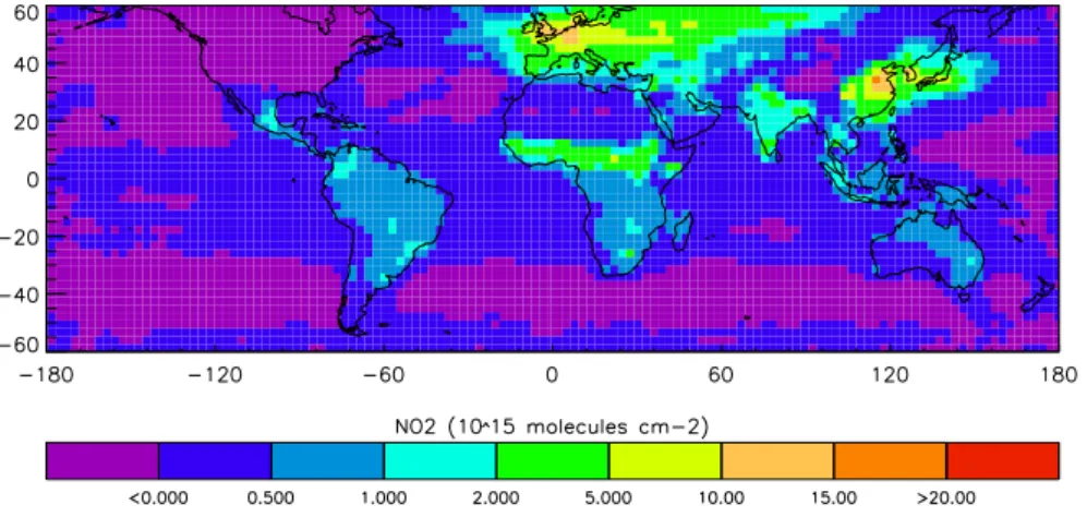
Fig. 5. Monthly mean tropospheric NO2 columns for January 1997 from the TOMCAT model (top), GOME retrieval (middle) and the percentage difference (bottom). Pixels where GOME is
<0.4×10¹⁵molec. cm−3are not plotted. The TOMCAT results are at the model resolution of 2.8×2.8◦while the GOME results have been averaged on to a 0.5×0.5◦grid. The differences are calcu-lated on the TOMCAT model grid. TOMCAT gives generally good agreement with the satellite data. The highest columns are correctly located and are of the right order of magnitude.
4 Results
Figures 5, 6 and 7 show January, July and September 1997 monthly mean column amounts of NO2 calculated from
GOME satellite measurements and TOMCAT. These figures show the GOME columns at 0.5×0.5◦degree resolution. The
Fig. 6. Monthly mean tropospheric NO2columns and percentage difference for July 1997. As for Fig. 5. The modelled NO2columns over Europe are substantially greater than GOME over Europe and the model also has greater concentrations over central Africa also.
modelled peak column densities are similar to the GOME column densities and are located in the same regions. Ac-cording to the Edgar 3.2 emissions inventory (Olivier et al., 2001) for 1995, 22% of all anthropogenic NOx emissions
were from the USA and Canada, with 13% from OECD Eu-rope and 25% from Asia. These areas with high anthro-pogenic NOxemissions can be seen as areas of high total
col-umn density. Other areas of high colcol-umns such as biomass burning regions can also be seen in both model results and the GOME data.
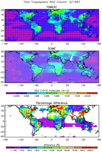
Fig. 7. Monthly mean tropospheric NO2columns and percentage difference for September 1997. As for Fig. 5. Note the region of high columns off the west coast of central Africa in the GOME results which may indicate a region of outflow. This is not seen in the TOMCAT results.
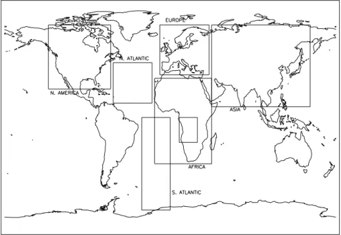
To examine in a more quantitative manner how well the model agrees with measurements for regions of high NO2
columns correlations were calculated on a region by region basis. These regions were defined as shown in Figure 8. To assess the significance of gradient of the correlations 2 ad-ditional estimates of the gradient are given. These are the ordinary least squares regressions from the sixlin procedure as described earlier calculated for the regression of x vs y (which gives a minimum estimate for the gradient) and y vs x (which gives a maximum estimate). Tables 2, 3 and 4 show the Pearson correlation coefficient and the gradient and inter-cept for all months for the regions where correlations were calculated.
The extent to which model results and GOME data agree has been examined by focusing in turn on: polluted re-gions; the North and South Atlantic; long range transport and African biomass burning.
4.1 Polluted regions
For July, especially over Europe, the modelled columns are much greater than the GOME data. For Europe the model columns are 100 to 200% greater than the GOME data – much larger than the retrieval error. Both the model and the GOME measurements show that the highest columns are found over northern Europe in the area of southern England, the Benelux countries and Germany. However the high con-centrations over northern Italy seen by GOME in January are not resolved by the model as its spatial resolution is too low. In contrast Velders et al. (2001) found that the modelled columns from the MOZART model were much higher than the measured values in January for Europe and agreed better with the GOME measurements over Europe for July. Lauer et al. (2002) tended to have larger European columns than GOME in both January and July which they attribute to the absence of a sink for N2O5on aerosol in their model.
Mar-tin et al. (2002) have better agreement than TOMCAT for July but in contrast to the TOMCAT model have lower NO2
columns over Europe than the GOME data. It must be noted however, that all these studies used different retrievals of GOME NO2as well as different models.
In Asia both TOMCAT and GOME have the highest columns over Japan and in China in the region around Bei-jing. Elevated columns are also seen over the Indian sub-continent. The modelled columns are again up to 200% greater than the GOME retrieval over polluter areas. Unlike in Western Europe however, the higher model columns can be seen in January as well as in the other months. The high-est columns over North America are on the East coast with some smaller peaks over the West Coast in the region around Seattle.
There are good correlations over polluted areas with mean values ranging from 0.71 for Asia to 0.89 for north Amer-ica. The reason why the correlation is better for more pol-luted regions may be that the emissions inventories for an-thropogenic emissions are more accurate because it is easier to estimate the regions of greatest emission and spatial ex-tent for anthropogenic emissions than for biomass burning and natural emissions. In the polluted regions the intercept for most months is small but the gradients vary widely. Mar-tin et al. (2002) found a correlation coefficient of 0.78 for the USA in July 1997 which is somewhat lower than the average value for North America obtained here of 0.93.
4.1.1 Seasonal cycles
The range of gradients during 1997 is the greatest over Eu-rope. The OLS bisector gradient is greater than 1 for all months except January and there is a distinct seasonal cy-cle in the gradients. The y vs x regression gradient (m-max) is only 0.83 in January while the x vs y regression gradi-ent (m-min) is 2.27 in summer. In the winter months the model is closest to a 1:1 correlation with the GOME data
Table 2. Correlations for Africa and Asia. r=correlation coefficient, m is OLS bisector gradient (model/satellite), m-min is OLS regression
x vs y, m-max is OLS regression y vs x, c is OLS bisector intercept. For more details see text.
Africa Asia
month r m m-min m-max c r m m-min m-max c
(molec. cm−3) (molec. cm−3) 1 0.82 1.23 1.01 1.52 −3.68E+14 0.67 1.09 0.73 1.65 1.54E+13 2 0.70 1.16 0.82 1.66 −5.04E+14 0.70 1.45 1.03 2.13 −4.14E+13 3 0.79 0.81 0.64 1.02 −1.51E+14 0.74 1.37 1.03 1.87 −1.99E+14 4 0.81 0.68 0.54 0.83 −7.08E+13 0.74 1.63 1.24 2.23 −2.89E+14 5 0.82 0.81 0.67 0.99 −2.09E+14 0.72 1.87 1.39 2.67 −4.35E+14 6 0.65 1.05 0.69 1.61 −1.21E+14 0.79 1.61 1.29 2.05 1.16E+14 7 0.73 1.68 1.25 2.37 −5.92E+14 0.70 1.62 1.17 2.38 −1.07E+14 8 0.73 1.61 1.20 2.27 −6.29E+14 0.71 1.77 1.29 2.58 −2.77E+14 9 0.68 1.41 0.98 2.14 −5.93E+14 0.64 1.77 1.19 2.93 −3.65E+14 10 0.76 0.96 0.72 1.26 −1.73E+14 0.77 1.80 1.42 2.37 −2.30E+14 11 0.72 1.77 1.32 2.51 −5.56E+14 0.82 1.44 1.19 1.77 −2.18E+14 12 0.86 1.56 1.34 1.83 −3.36E+13 0.53 0.86 0.44 1.58 2.53E+14
Mean 0.76 1.23 0.93 1.67 −3.33E+14 0.71 1.52 1.12 2.19 −1.48E+14
Table 3. Correlations for Europe and North America. As Table 2.
Europe N. America
month r m m-min m-max c r m m-min m-max c
(molec. cm−3) (molec. cm−3) 1 0.74 0.62 0.45 0.83 1.69E+15 0.86 0.99 0.85 1.16 2.98E+14 2 0.66 1.47 1.01 2.30 1.11E+15 0.82 1.25 1.03 1.55 1.65E+14 3 0.84 1.63 1.37 1.97 8.91E+13 0.91 1.41 1.28 1.57 −7.02E+13 4 0.79 1.58 1.26 2.04 9.62E+14 0.93 1.42 1.32 1.52 −1.11E+14 5 0.75 2.62 2.03 3.59 6.43E+13 0.88 1.83 1.62 2.07 −2.27E+14 6 0.68 3.14 2.27 4.89 −1.00E+15 0.90 1.52 1.37 1.68 −2.30E+14 7 0.79 2.97 2.40 3.85 −1.77E+15 0.90 1.61 1.45 1.79 −5.06E+14 8 0.90 2.42 2.18 2.72 −1.11E+15 0.89 2.06 1.84 2.32 −7.93E+14 9 0.86 1.86 1.61 2.17 −4.24E+14 0.90 1.94 1.76 2.16 −4.83E+14 10 0.86 1.74 1.51 2.03 2.12E+14 0.92 1.80 1.67 1.96 −2.37E+14 11 0.85 1.51 1.28 1.79 6.20E+14 0.92 1.38 1.27 1.50 5.66E+13 12 0.73 1.20 0.89 1.66 5.77E+14 0.85 1.64 1.40 1.94 −4.42E+13
Mean 0.79 1.90 1.52 2.49 8.50E+13 0.89 1.57 1.40 1.77 −1.82E+14
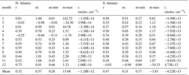
Table 4. Correlations for North and South Atlantic. As Table 2.
N. Atlantic S. Atlantic
month r m m-min m-max c r m m-min m-max c
(molec. cm−3) (molec. cm−3) 1 0.01 1.00 0.01 142.72 −1.03E+14 0.58 0.51 0.27 0.81 −9.50E+13 2 −0.02 −0.98 −0.01 −34.30 3.99E+14 0.33 0.52 0.12 1.12 −1.36E+14 3 0.01 0.99 0.01 44.78 −3.30E+14 0.37 0.57 0.16 1.18 −9.15E+13 4 0.39 0.70 0.23 1.51 −1.38E+14 0.50 0.65 0.29 1.17 −7.92E+13 5 −0.25 −0.66 −0.11 −1.76 3.98E+14 0.74 0.39 0.28 0.51 −8.84E+13 6 0.53 0.53 0.25 0.89 −4.11E+13 0.48 0.38 0.15 0.64 −2.78E+13 7 0.55 0.74 0.39 1.26 −1.51E+14 0.58 0.43 0.23 0.67 −1.47E+12 8 0.55 0.82 0.43 1.44 −1.04E+14 0.80 0.32 0.25 0.39 −7.86E+13 9 0.49 0.79 0.36 1.52 −8.61E+13 0.53 0.29 0.13 0.46 −6.46E+13 10 0.44 1.01 0.45 2.28 1.29E+13 0.58 0.24 0.13 0.37 −4.23E+13 11 0.42 1.06 0.45 2.61 2.09E+13 0.18 0.46 0.04 1.07 −8.81E+13 12 0.73 0.91 0.66 1.23 1.06E+14 −0.01 −0.98 0.00 −54.33 4.73E+13
Fig. 8. Map of all regions used for analysis. The Central Africa region is the small box entirely inside the Africa region.
Fig. 9. Scatter plot of tropospheric NO2columns TOMCAT results versus GOME retrieval. Europe, June 1997. Thin line 1:1 ratio, thick line least squares fit. Although the TOMCAT results are well correlated with the satellite data, a large fraction of the points are above the 1:1 line and the best fit has a gradient of 3.14.
while the largest OLS bisector gradient (3.14) is calculated in June. The gradient of 3.14 is consistent with the global plot which shows TOMCAT having a colimn 200% greater than GOME for this region. Figure 9 shows a scatter plot of modelled columns versus GOME retrievals over Europe in June 1997. It can be seen that the majority of points lie well above the 1:1 line.
Further evidence for this strong seasonal difference is found when the mean column over Europe is calculated from
Fig. 10. Seasonal cycle of average tropospheric NO2columns over Europe as calculated by TOMCAT (middle line, in blue) and from GOME data (lower line, in red). Error bars indicate the standard deviation of the column over the area. The TOMCAT/GOME ratio is in green. The TOMCAT columns are higher than the GOME values for all months and also decrease less in the summer months compared to winter.
the TOMCAT data and using the GOME data re-gridded onto the TOMCAT model grid (Fig. 10). The error bars are the standard deviation of the column over this area. Note that the error bars on this plot do not represent a model or retrieval error but the variation in columns over the region. A perfect model would be able to reproduce not just the average col-umn but this variability. It therefore inappropriate to assume
that because the model and GOME errors overlap the differ-ences in the results are statistically insignificant. On average over Europe the mean TOMCAT column is between 1.1 and 2.7 times higher than GOME which is much larger than the retrieval error and in general agreement with the relative dif-ference found earlier in the global plots for this region. This difference is the highest in the late spring and early summer months. The seasonal cycle in TOMCAT is qualitatively cor-rect though with a minimum in the summer months. The model has a larger standard deviation than the measurements in the summer, while in January when the TOMCAT mea-surements are the closest to the GOME data, the standard deviation is smaller. This is similar to the results of Lauer et al. (2002) for Europe, but the gradient of the regression here is much less than in that study. However that study used a GCM with only a preliminary tropospheric NOxchemistry.
A similar but less pronounced pattern is seen for Asia and North America. Both have only one month where the gradi-ent of the correlation is less than 1. The highest correlations in both are also in the summer months (August for North America, May for Asia). However the maximum OLS bisec-tor gradients are lower – 1.74 for North America and 1.86 for Asia. Kunhikrishnan et al. (2004) found that model-GOME agreement was not consistent in all Asian sub-domains with India having the worst agreement and the model failing to capture the biomass burning peaks for North Asia and China. If smaller domains were used for the analysis it might im-prove the agreement for some areas.
In summary, there is a high correlation between GOME data and TOMCAT results for polluted regions with high NO2columns but the model results tend to have higher
con-centrations in these areas than the data especially in summer. 4.2 Contrast between North and South Atlantic
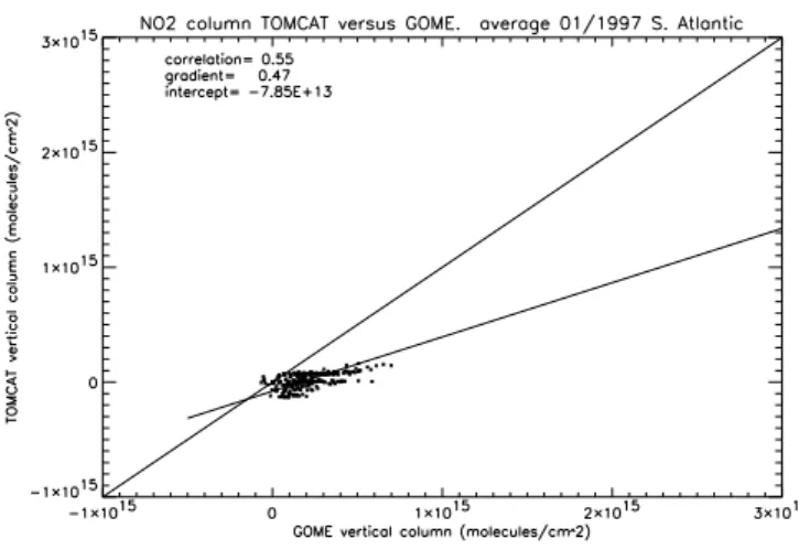
The oceanic regions have much lower correlations and OLS bisector gradients which are very small compared to those over source regions. The lower correlations might be ex-pected as the concentrations are lower and the range of val-ues is smaller, thus the impact of errors will be greater. There is also a major difference between the North and South At-lantic. As well as having a smaller correlation, the North Atlantic has a higher mean gradient (despite 2 months where it has a large negative gradient).
Figures 11 and 12 show scatter plots of TOMCAT versus GOME for the North and South Atlantic respectively. These figures show why there is such a difference in the correla-tions and gradients in the two regions. The South Atlantic (Fig. 11) has a single population of data with all modelled values low and most below the 1:1 line. It would appear that in this region which is remote from most anthropogenic influence the modelled concentrations are much lower than GOME. We can see these lower concentrations in the plots of the global data also. In contrast, there seem to be two dis-tinct populations in the North Atlantic (Fig. 11), one of low
Fig. 11. Scatter plot of tropospheric NO2columns TOMCAT results versus GOME retrieval. For South Atlantic January 1997. As Fig. 9. In contrast to the scatter plot for Europe, over the south Atlantic a large proportion of the TOMCAT points are below the 1:1 line.
Fig. 12. Scatter plot of tropospheric NO2columns TOMCAT results versus GOME retrieval. For North Atlantic January 1997. As Fig. 9. This scatter plot shows how there appear to 2 populations of data in the North Atlantic: one similar to the South Atlantic and another above the 1:1 line which is closer to the European population.
values similar to the South Atlantic and a second which is much higher. These two populations cause the correlation to be lower and also give larger gradients for most months. 4.3 Long range transport of NOy
Nitrogen oxides are among the compounds which are con-trolled by the UNECE Convention on Long-range Trans-boundary Air Pollution and so measurements and the vali-dation of models of global transport of nitrogen oxides are highly important. As a precursor to tropospheric ozone for-mation long range transport of NOxis also key to
Fig. 13. Tomcat tropospheric NO2column for January 1997 without North American Anthropogenic emissions. This shows how without N. American emissions the band starting from the east coast of the USA is not present, giving strong evidence that this feature is due to the export of North American emissions.
changing sources and sinks along air mass trajectories. For example, in the upper troposphere, NOx concentrations can
be enhanced by in situ emissions (e.g. lightning) or injection of polluted air masses from the surface or by chemical pro-cesses such as photolysis of HNO3which recycle NOxfrom
reservoir species.
The source regions considered here are North America where anthropogenic emissions are carried eastwards over the Atlantic, and the westward transport of African biomass burning emissions. It would be useful to be able to exam-ine the fate of European emissions but this is complicated by the fact that they are not carried over an oceanic region by prevailing winds and so further NOxemissions occurring
downwind complicate any examination of outflow from this region. In addition, in winter when the plumes are the most obvious, the region to the east of Europe is very cloudy and there is little or no GOME data for the region downwind of Western Europe in these months. Clouds may also introduce extra uncertainty because many export events are associated with cloud and so will not be observed in this GOME re-trieval.
4.3.1 Export from North America into the Atlantic Figure 12 may show the influence of plumes of NO2on the
correlations in the North Atlantic region. In the global model plots for January (Figure 5) and to a lesser extent in July and September (Figs. 6 and 7) we can see a band of elevated concentrations which stretches in a generally northeastward direction from the east coast of the US towards Europe. How-ever this also coincides with a region of both high shipping and aircraft emissions so it is not possible to assign this re-gion of elevated concentrations solely to export.
In January (Fig. 5) the concentrations in this region are much higher in TOMCAT than those indicated by the satel-lite results. This is not a result of different source strengths alone as the NO2 concentrations over the east coast of the
USA are approximately the same in both sets of data. This contrast between the model and satellite data is not how-ever consistent between months. For example in Septem-ber (Fig. 7) it can be seen that the total column of NO2over
the North Atlantic in the satellite data is similar to that of the model. In July (Fig. 6) if anything the model is slightly lower than the GOME data. In both July and September the modelled concentrations over the east coast of the US are too high so the agreement over the Atlantic again suggests that there may be a problem with the way this export is modelled either in terms of transport of chemistry.
There are a large number of processes occurring in this re-gion which can have an impact on the concentrations of NO2.
Various studies have shown that warm conveyor belts asso-ciated with frontal systems are an important mechanism for transporting emissions from the north east of north America out across the Atlantic. For more details of these flows see Stohl (2001). NO2also has a secondary source from HNO3
and PAN as well as in situ production from lightning and emissions from ships and aircraft.
In order to examine the possibility that the NO2 in this
region is primarily a result of in situ emissions (either an-thropogenic or lightning) the model was rerun without any anthropogenic emissions of NOxfrom North America.
Fig-ure 13 shows the results of this experiment for January. When there are no North American emissions, the high concentrations in the North Atlantic are absent. The non-linearity of the O3 – NOx chemistry may mean that ozone
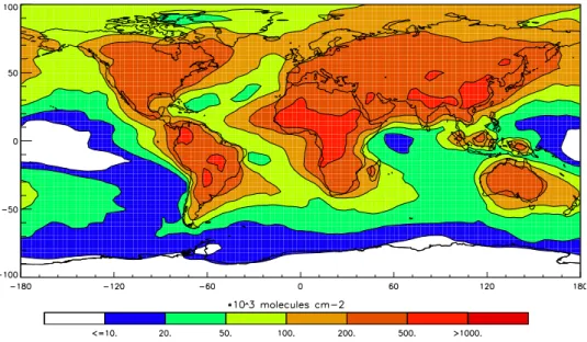
Fig. 14. Total column of Radon from the TOMCAT model September 1997. The regions of outflow from North America, Asia and Africa
can all be seen in the radon column.
OH production is also therefore possibly inhibited and so this is not a fully quantitative method for examining the contri-bution of North American emissions to the total NO2
col-umn. However if the OH concentration is reduced then in-situ emissions will have a longer lifetime and so contribute a larger column in the middle of the Atlantic.
4.3.2 Export from Africa by easterly winds
Elevated NO2columns with the appearance of plumes from
Africa can be seen in the GOME data off the coast of Africa in the region of easterly winds for January (Fig. 5), July (Fig. 6) and September (Fig. 7). In January this apparent export can be seen from west Africa into the Atlantic in the GOME data but in the TOMCAT data this plume ends very close to the coast. Unlike in the mid-latitude plumes, the model consistently has lower concentrations in the region of these plumes whether they start from West Africa (in Jan-uary) or from Central Africa (in July and September). The absence of this export in the model may be part of the reason why the correlation in the South Atlantic has such a low gra-dient. However these differences between the model and the data are close to or less than retrieval error and so retrieval error can not be ruled out as an explanation.
One explanation which must be considered is that these elevated columns are not primarily the result of plumes of biomass burning emissions but are from NOxproduction by
lightning. However, the columns off the coast do seem to be consistent with the elevated concentrations over regions with high biomass burning emissions. The most clear exam-ple of this in the GOME data is September when the highest
columns are seen over central Africa and the largest columns over the west coast of central Africa are also seen. The sea-sonal signal of lightning flash frequency is the reverse of that for biomass burning (see for example Jourdain and Hauglus-taine, 2001) with a high flash frequency over west Africa in July and higher in southern and central Africa in January and so it seems unlikely that lightning can explain these features. However, some of the elevated concentrations in July over west Africa may be attributed to lightning.
Too fast vertical transport of NO2in the model could mean
that, instead of NO2being transported mainly at low levels
to the West, in the model it is transported at higher levels to the East. Another plausible explanation for the model not re-producing the observed export of NO2from Africa into the
Atlantic is that this circulation is not correctly represented in the model. With a half life of 3.8 days and a source which is dominated by terrestrial sources, radon is a useful tracer for considering these questions. Figure 14 shows the total col-umn of radon for September 1997. The westward transport of air from West Africa can be clearly seen in this figure and, although not as strong, advection of air from Central Africa over the Atlantic is also visible. If the westward transport of air is reproduced for radon then it will be reproduced for other model tracers as well. This suggests that an incorrectly modelled westward advection or too fast vertical transport affecting the direction of outflow are unlikely to be major reason why elevated NO2 columns are not observed in this
region in the model results. To test in more detail how well the advection in this region is modelled would require pro-files of radon or another short-lived tracer to be measured in this region.
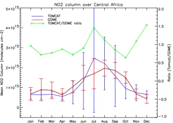
Fig. 15. Seasonal cycle of average tropospheric NO2columns over Central Africa as calculated by TOMCAT model (in blue) and from GOME data (in red). Error bars indicate the standard deviation of the column over the area. The TOMCAT/GOME ratio is in green. In comparison to Europe the TOMCAT columns agree much bet-ter with the GOME columns. However, the peak in the TOMCAT column is earlier and higher than for GOME. In addition during the period of high columns the standard deviation is much greater for the TOMCAT results than in the GOME data.
4.4 Biomass burning distribution and seasonal cycle The main region of biomass burning over West Africa in Jan-uary is a region with elevated NO2columns in both the model
and the GOME data and in January the model and satellite data agree to within the retrieval error for most pixels. The area where this region of elevated columns (probably a result of biomass burning emissions) is located in the model fol-lows closely that observed by the satellite data, with a south-ward movement of the areas of elevated columns through the year due to the seasonality in the position of the ITCZ as has been documented previously e.g. Hao and Liu (1994) and can also been seen from the ATSR firecount data (see Figs. 2 and 4). In the region near the west coast of Africa from the equa-tor to about 20◦south (described as central Africa in this pa-per) elevated NO2from biomass burning can be clearly seen
in July in both the model and the GOME data (see Fig. 6). The minimum values of the OLS gradients over Africa are in April (0.54–0.83) and the maximum (1.32–2.51) are in November. This is a completely different seasonal cycle to that found for the mid-lattitude polluted regions. Apart from the months of March to May, when biomass burning is at a minimum in Africa, the gradient of the correlations are greater than 1 but are within the GOME retrieval errors for months. In the global plot for July (Fig. 6) however, the columns in the regions of high concentrations are up 200% greater in the model than in the satellite data for the central Africa region.
In order to examine how well the model captures seasonal variations in biomass burning emissions, it is useful to con-sider a smaller area than in the previous correlations. Central Africa (9.8–29.5◦longitude, 0 to −19.5◦latitude) was cho-sen, because Figs. 5, 6 and 7 show that the seasonal changes are strongest in this region. The seasonal cycle is shown in Fig. 15.
The model agrees very well with the GOME data for the majority of months and the general timing and amplitude of the seasonal cycle are approximately correct especially when the large variability in this area in both the model and the measurements is taken into account. It could be argued that the peak in modelled NO2concentrations is somewhat earlier
and more intense when compared to the peak concentrations in GOME. TOMCAT’s peak concentrations are in July and are greater than in the peak in GOME data which occurs in August. The elevated concentrations in GOME persist until October while the TOMCAT columns fall off more quickly. The variability of TOMCAT data in this region is also larger than the variability of the measurements during this peak, whereas earlier in the year it is smaller than observed. Law et al. (2000) have shown using ozone measurements from the MOZAIC program in the upper troposphere over central Africa that TOMCAT and several other CTMs do not exactly capture the seasonal cycle of biomass burning emissions in this region. However given the uncertainties in the GOME data and the high variability of both model and satellite data the model seems to be in generally good agreement for this region. If a emission inventory based on fire count data for 1997 were to be used in the model it might be expected that the model agreement with GOME and MOZAIC data could be further improved.
5 Discussion
Clearly, a single model deficiency cannot explain all of the features discussed above. In fact, each of the model discrep-ancies may be a result of several limitations acting together. It is therefore useful to consider each of the processes affect-ing the concentrations and distribution of NO2in turn and the
limitations in modelling these processes which could lead to such differences.
5.1 Emissions
As the major source of NOxis from surface emissions they
play a key role in determining the modelled concentrations. The good correlations for the winter months in polluted re-gions suggests that the distribution of emissions used to pro-duce emission inventories for industrial emissions are un-likely to a major source of GOME-TOMCAT differences. Overestimated emissions from polluted regions could par-tially explain the large over-prediction of model columns over Europe and other polluted regions but there is no other
evidence to suggest that the emission inventories have such a large error. Given that for this inventory industrial emissions were scaled to be appropriate for 1997, trends in emissions are unlikely to have played a significant role in differences between TOMCAT and GOME results. Fossil fuel emissions are estimated (Olivier et al., 2003) to have a medium total un-certainty (of the order of 50%) which strongly suggests that errors in the emissions alone cannot explain this discrepency. As regards the seasonal cycle of differences over Europe, North America and Asia, the lack of a seasonal cycle in the emission inventory used for industrial emissions may play a role in model – GOME discrepancies. Industrial NOx
emis-sions are lower in the summer as a result in particular of lower energy requirements for space heating and lighting. However, in the Northern Hemisphere regional emissions only vary by up to 15% from a uniform distribution (Olivier et al., 2003) and so seem unlikely as the major explanation for the differences in the modelled and observed seasonal cy-cle of NO2columns. Also of possible importance are daily
cycles of emissions, especially the potential importance of rush hour peaks in NOx emissions. At higher model
reso-lutions these cycles will probably increase in importance as there will be less model-induced “smearing” of emissions. 5.2 Physical processes
The major physical processes which play a role in the distri-bution of NO2are large scale horizontal transport, dry
depo-sition and vertical mixing. 5.2.1 Vertical mixing
When considering the effect of vertical mixing in the model it is important to note that the model profile of NO2affects
the GOME retrieval. This is because the Air Mass Factor used to convert from slant column data to vertical columns is calculated based on an a-priori NO2profile from TOMCAT.
The effect of increased vertical mixing either in the bound-ary layer or due to stronger convection would decrease the fraction of modelled NO2close to the ground thus meaning
that the NO2column retrieved from the GOME observations
would be decreased. Increased vertical mixing in the model would also increase the total modelled column as the lifetime of NO2is less at low level. Increased vertical mixing in the
model therefore decreases the GOME columns and increases the modelled columns. This implies that GOME-TOMCAT comparisons are especially sensitive to errors in the modelled vertical transport and so are potentially a rigorous test of the model. Convection and boundary layer mixing are very vari-able in time and space. This means that this study, which uses monthly mean data, is limited in its ability to evaluate in detail these issues. The same convective mixing scheme was tested in Stockwell et al. (1998) using a previous version of the TOMCAT model by comparison with observed pro-files of radon. That model version used a local vertical
diffu-sion scheme (Louis, 1979) and there was insufficient vertical mixing near the surface. The boundary layer mixing in the model has since been improved by the use of a non-local ver-tical diffusion scheme (Holtslag and Boville, 1993) as docu-mented in Wang et al. (1999). The model now shows much better agreement with the profiles discussed in Stockwell et al. (1998). The boundary layer mixing gives concentrations near the surface which are much closer to the observations.
If the summertime convection over Europe were too strong in the model this would explain the overestimation by TOM-CAT of the NO2columns. A comparison of TOMCAT
pro-files with aircraft observations over central Europe in the EX-PORT campaign (e.g. O’ Connor et al., 2004) seems to indi-cate that the modelled boundary layer concentrations of NO2
are too low (probably because the model is unable to resolve local sources) and concentrations in the free troposphere are approximately correct. Brunner et al. (2003) found that for most parts of the free troposphere TOMCAT had a negative bias for NOxwhen compared to the results of aircraft
obser-vations. This makes it difficult to come to any clear conclu-sions on whether vertical mixing is the major process causing model-GOME differences.
If the modelled convection over tropical oceans is too weak in the model this might explain the lower NO2columns
calculated off the coast of West Africa compared to GOME results. Too little convective activity over oceans in the model might also provide an explanation for the low gradi-ents (mean of 0.31) observed over the south Atlantic. How-ever there is some evidence that the convection over land as modelled in TOMCAT is too weak while that over the oceans is too strong. This again suggests that incorrect vertical mix-ing does not explain the differences between modelled and satellite NO2 columns. The modelled export of emissions
from source regions would also be underestimated if convec-tive processes over land in the model were to be too weak. Too little convection would cause less of the NO2to reach
high levels where more rapid horizontal transport occurs and where the NOxlifetime is longer. If export from polluted
re-gions is too weak in TOMCAT, due to weak convection over the land this would partially explain the low concentrations off the west coast off Africa.
The question of vertical mixing in chemistry-transport models is one which deserves further work and this would best be addressed by an approach which combined satellite and aircraft measurements in a series of well chosen case studies.
5.2.2 Dry deposition
NO2 is dry deposited at the surface. The deposition
veloc-ity is not large so this is unlikely to be a cause of model-measurement differences. Nevertheless, if the dry deposi-tion in the model is too strong it could affect both the mod-elled NO2column and the retrieval. Increasing dry
also change the vertical profile of NO2. A smaller fraction
of the NO2near the surface would change the Air Mass
Fac-tor calculated from the model data and so reduce the column density in the GOME retrieval because the retrieval is less sensitive to NO2at lower levels. Unlike for changes in
verti-cal transport therefore the satellite-model comparison is rel-atively insensitive to errors in the modelled dry deposition. 5.3 Chemistry
The two main limitations in the model chemistry scheme which might explain the differences between the model and GOME data are the limited number of hydrocarbons in the model and, in particular, the absence of isoprene chemistry. These enhancements of the model chemistry would favour rapid formation of PAN and higher homologues in the bound-ary layer. This could result in lower NO2concentrations over
polluted areas as well as higher columns in regions where the air is descending when NO2is subsequently released due
to thermal decomposition. Any other missing gas phase or multi-phase reactions of oxides of nitrogen would be a part explanation of the differences between model and GOME NO2. It is quite likely that there are different weaknesses in
the model chemistry scheme in the marine boundary layer, the polluted boundary layer and the free troposphere. 5.4 Model resolution
The low resolution of the model will cause rapid mixing of emissions and so tend to reduce the concentrations of the highest peaks and increase the concentrations over the more remote regions. However it is not clear from the correla-tion plots that this is a major issue The model uses an ad-vection scheme which preserves gradients reasonably well. In addition in regions of high emissions, NO may remove most of the ozone, thus creating a high NO/NO2ratio. This
would not be observed in the model results if regions of high emissions are smeared out in the model. This could lead to the model having too much NO2and might help explain the
larger NO2columns in the model over polluted areas.
5.5 Cloud effects on model results
In the GOME retrieval used for this study cloudy pixels are not used to calculate the tropospheric NO2column. This
in-troduces an inconsistency between the model and measure-ments. In TOMCAT photolysis rates in the model are calcu-lated using latitudinally averaged cloud climatologies. This means that the photolysis rates of NO2in the model are lower
than those in the real atmosphere where the GOME measure-ments are made (as only cloud free pixels are included). It might be expected that this lower modelled photolysis rate would lead to a higher NO2/NOxratio in the model thus
po-tentially explaining part of the positive bias of the modelled values over polluted regions. However, this cannot explain the difference in seasonality between TOMCAT and GOME
over polluted regions. As the cloudiness is greatest in winter this would imply that the model should have a stronger posi-tive bias in the winter months whereas in fact this is when the best agreement is found. An estimate of the order of magni-tude of this effect can be found by taking the ratio of photol-ysis rates calculated for cloudy to non-cloudy scenarios. For a latitude of 53◦N in June this ratio is 0.82. This means that this is potentially a significant effect but cannot alone explain the model-GOME differences.
Cloud effects may explain part of the observed difference between model and measurement with respect to export of NO2 from the US and Europe, as GOME might
systemati-cally be unable to observe export events because of enhanced cloudiness. It might also help explain some of the differences between model performance for Europe and the US. Cloudi-ness is likely to be a greater problem for Europe than over the whole of North America.
To remove this bias from the model would require 2 changes to the methods used here. Firstly a photolysis scheme coupled to cloudiness data input from the meteoro-logical analyses would have to be included in the model. In addition, it would be necessary to sample the model at the time and place of each GOME measurement used to calcu-late the monthly mean instead of using the monthly mean model column at 10:30 local time. This would also address other potential factors arising from the fact that the GOME measurements are only for cloud free pixels such as differ-ences in wind speed and direction and convection.
In addition for Europe in winter there is lack of represen-tativeness due to the loss of data from cloud screening. This may contribute in part to the particularly strong seasonal dif-ferences over Europe between model and GOME.
6 Conclusions
The successful modelling of tropospheric NOx is a major
challenge for CTMs (e.g. Brunner et al., 2003). Given that, the TOMCAT model is overall in reasonably good agreement with the GOME data but has a positive bias relative to GOME with a correlation coefficient of 0.79 and a gradient of 1.5 for the whole world. The region with the best agreement with the GOME data is in Africa for most months of the year and in the polluted Northern Hemisphere in winter. How-ever three main areas of disagreement have been found: the seasonal cycle of NO2columns over polluted areas, regions
of pollution export over oceans and the exact distribution and intensity of biomass burning distributions. Future model de-velopment activities should consider GOME NO2 data as a
highly important set data for testing any changes made to models and new emission inventories. The most important explanations for disagreements between the model and mea-surements seem likely to be limitations in the model chem-istry scheme and limitations in the vertical transport schemes (convection and boundary layer) and biases introduced by the
use of monthly mean model results instead of sampling the model at the location of GOME pixels.
Possible methods for improving the performance of the TOMCAT model include: including seasonal cycles in an-thropogenic emissions; better treatment of clouds; additional NMHC chemistry, especially that of isoprene, and a param-eterisation for N2O5loss on aerosol. Also the use of
multi-annual model runs will allow the variability of these model-GOME differences to be considered which will hopefully also provide further insight into the atmospheric chemistry of NO2in both the model and the real atmosphere. It would
also be worth comparing multiple models to the same set of GOME data in a single study to allow a better compari-son of how well different models are able to reproduce the NO2 columns. Higher resolution simulations with
TOM-CAT would allow the effect of model resolution to be exam-ined. A new parallel version of the model has been developed and this will allow additional chemistry and other model im-provements in the future. Finally, case studies of specific events such as Warm Conveyor Belts (Stohl, 2001) or a “me-teorological bomb” (Stohl et al., 2003) could provide valu-able insight into how well transport pathways from polluted areas are modelled. Other case studies should concentrate on periods where there is satellite data coincident with an air-craft campaign. To investigate the effects of cloudiness on the GOME-model comparison would require an on-line pho-tolysis scheme in the model and the sampling of the model at the time and place of each GOME measurement rather than simply using data output at 10:30 local time.
Acknowledgements. This work was carried out as part of the
European Union funded program POET (ENVK2-CT1999-00011) and was funded in part by the University of Bremen, German Aerospace Agency (DLR) and the German Ministry for Education and Research (BMBF). Funding and supercomputer support was also provided by the NERC Centres for Atmsopheric Science. The authors would like to thank M. Chipperfield for providing SLIMCAT model data and R. Koelemeijer for making the surface reflectivity data base available. The authors would like to thank F. O’Connor for her advice and comments on the text. The authors also acknowledge the ECMWF for allowing access to their meteorological analyses and the British Atmospheric Data Centre (BADC) for supplying them. The authors acknowledge NCAR for supplying the planetary boundary layer scheme from their Community Climate Model (CCM2). The authors also wish to thank ATSR World Fire Atlas, European Space Agency – ESA/ESRIN, via Galileo Galilei, CP 64, 00044 Frascati, Italy for the ATSR firecount data. Finally we would like to thank both reviewers for their useful comments.
Edited by: F. Dentener
References
Boersma, K. F., Eskes, H. J., and Brinksma, E. J.: Error Analysis for Tropospheric NO2Retrieval from Space, J. Geophys. Res., 109, D04311, doi:10.1029/2003JD003962, 2004
Borrell, P., Builtjes, P., Genfelt, P., and Hov, Ø.: Photo-Oxidants, Acidification and Tools: Policy Applications of Eurotrac Results, Springer-Verlag Berlin Heidelberg, ISBN 3-540-61783-3, 1997. Brunner, D., Staehelin, J., Rogers, H. L., K¨ohler, M. O., Pyle, J. A., Hauglustaine, D., Jourdain, L., Berntsen, T. K., Gauss, M., Isak-sen, I. S. A., Meijer, E., van Velthoven, P., Pitari, G., Mancini, E., Grewe, V., and Sausen, R.: An evaluation of the performance of chemistry transport models by comparison with research aircraft observations, Part 1: Concepts and overall model performance, Atmos. Chem. Phys., 3, 1609–1631, 2003,
SRef-ID: 1680-7324/acp/2003-3-1609.
Burrows, J. P., Weber, M., Buchwitz, M., Rozanov, V., Ladst¨atter-Weißenmayer, A., Richter, A., DeBeek, R., Hoogen, R., Bram-stedt, K., Eichmann, K.-U., Eisinger, M., and Perner, D.: The Global Ozone Monitoring Experiment (GOME): Mission Con-cept and First Scientific Results, J. Atmos. Sci., 56, 151–175, 1999.
Carver, G. D., Brown, P. D., and Wild, O.: The ASAD atmospheric chemistry integration package and chemical reaction database, Comput. Phys. Commun., 105, (2–3), 197–215, 1997.
Chameides, W. L., Fehsenfeld, F., Rodgers, M. O., Cardelino, C., Martinez, J., Parrish, D., Lonneman, W., Lawson, D. R., Ras-mussen, R. A., Zimmerman, P., Greenberg, J., Middleton, P., and Wang, T.: Ozone Precursor Relationships in the Ambient Atmo-sphere, J. Geophys. Res., 97, D5, 6037–6055, 1992.
Chipperfield, M. P.: Multiannual Simulations with a Three-Dimensional Chemical Transport Model, J. Geophys. Res., 104, 1781–1805, 1999.
ESA (European Space Agency): GOME Global Ozone Monitoring Experiment users manual, ESA SP-1182, ESA/ESTEC, Noord-wijk, Netherlands, ISBN 92-9092-327-x, 1995.
Eskes, H. J. and Boersma, K. F.: Averaging kernels for DOAS total-column satellite retrievals, Atmos. Chem. Phys., 3, 1285–1291, 2003, SRef-ID: 1680-7324/acp/2003-3-1285.
Grewe, V., Brunner, D., Dameris, M., Grenfell, J. L., Hein, R., Shin-dell, D., and Staehelin, J.: Origin and variability of upper tro-pospheric nitrogen oxides and ozone at northern mid-latitudes, Atm. Env., 35, 20, 3421–3433, 2001.
Haagen-Smit, J. A.: Chemistry and physiology of Los Angles smog, Ind. Eng. Chem., 44, 1342–1346, 1952.
Hao, W. M. and Liu, M. H.: Spatial and Temporal distribution of tropical biomass burning, Global Bigechem. Cyc., 8, (4), 495– 503, 1994.
Holtslag, A. A. M. and Boville, B. A.: Local versus nonlocal bound-ary layer diffusion in a global climate model, J. Clim., 6, (10), 1825–1842, 1993.
Houghton, J. T., Ding, Y., Griggs, D. J., Noguer, M., van der Lin-den, P. J., and Xiaosu, D. (Eds.): Climate Change 2001: The Scientific Basis Contribution of Working Group I to the Third Assessment Report of the Intergovernmental Panel on Climate Change (IPCC), Cambridge University Press, UK, 2001. Isobe, T., Feigelson, E. D., Akritas, M. G., and Babu, G. J.: Linear
Regression in Astronomy, I. Astrophysical J., 105, (2–3), 197– 215, 1990.