HAL Id: hal-00814659
https://hal-pjse.archives-ouvertes.fr/hal-00814659
Preprint submitted on 17 Apr 2013HAL is a multi-disciplinary open access archive for the deposit and dissemination of sci-entific research documents, whether they are pub-lished or not. The documents may come from teaching and research institutions in France or
L’archive ouverte pluridisciplinaire HAL, est destinée au dépôt et à la diffusion de documents scientifiques de niveau recherche, publiés ou non, émanant des établissements d’enseignement et de recherche français ou étrangers, des laboratoires
Poverty and Well-Being: Panel Evidence from Germany
Andrew E. Clark, Conchita d’Ambrosio, Simone Ghislandi
To cite this version:
Andrew E. Clark, Conchita d’Ambrosio, Simone Ghislandi. Poverty and Well-Being: Panel Evidence from Germany. 2013. �hal-00814659�
WORKING PAPER N° 2013 – 08
Poverty and Well-Being: Panel Evidence from Germany
Andrew E. Clark Conchita d'Ambrosio
Simone Ghislandi
JEL Codes : I31, D60
Keywords: Income; Poverty; Subjective well-being; SOEP
P
ARIS-
JOURDANS
CIENCESE
CONOMIQUES48, BD JOURDAN – E.N.S. – 75014 PARIS TÉL. : 33(0) 1 43 13 63 00 – FAX : 33 (0) 1 43 13 63 10
Poverty and Well-Being:
Panel Evidence from Germany
*A
NDREWE.
C
LARK Paris School of Economics - CNRSC
ONCHITAD’A
MBROSIOUniversità di Milano-Bicocca, DIW Berlin and Econpubblica [email protected]
S
IMONEG
HISLANDI Università Bocconi and Econpubblica [email protected]This version: March 2013
Abstract
We consider the link between poverty and subjective well-being, and focus in particular on the role of time. We use panel data on 42,500 individuals living in Germany from 1992 to 2010 to uncover four empirical relationships. First, life satisfaction falls with both the incidence and intensity of contemporaneous poverty. There is no evidence of adaptation within a poverty spell: poverty starts bad and stays bad in terms of subjective well-being. Third, poverty scars: those who have been poor in the past report lower life satisfaction today, even when out of poverty. Last, the order of poverty spells matters: for a given number of poverty spells, satisfaction is lower when the spells are concatenated: poverty persistence reduces well-being. These effects differ by population subgroups.
Keywords: Income, Poverty, Subjective well-being, SOEP. JEL Classification Codes: I31, D60.
* We thank Markus Grabka, Peter Krause, Nico Pestel and seminar participants at IARIW (Boston),
Duisburg-Essen, Keio, Manchester, Osaka and VID (Vienna) for many valuable suggestions. The German data used in this paper were made available by the German Socio-Economic Panel Study (SOEP) at the German Institute for Economic Research (DIW), Berlin: see Wagner et al. (2007). Neither the original collectors of the data nor the Archive bear any responsibility for the analyses or interpretations presented here.
1. Introduction
The relationship between an individual's income and their subjective well-being has been the focus of much empirical work, both within and across countries, and both at a single point in time and over time. This existing research has come to three main conclusions: 1) within each country at a given point in time, richer people are more satisfied with their lives, with additional income increasing satisfaction at a decreasing rate; 2) within each country over time, an increase in average income does not substantially increase satisfaction with life; and 3) across countries, on average, individuals living in richer countries are more satisfied with their lives than are those living in poorer countries (see, amongst many others Blanchflower and Oswald, 2004, Clark et al., 2008b, Diener and Biswas-Diener, 2002, Di Tella and MacCulloch, 2006, Easterlin, 1995, Frey and Stutzer, 2002, and Senik, 2005).
While there is now something of a consensus with respect to the above, it is noteworthy that the majority of the analysis in this burgeoning subjective well-being literature has been resolutely atemporal (whereby some measure of current well-being is related to current income), with relatively few exceptions which we will discuss below. However, at the same time, a considerable amount of recent work in various fields of Economics has underlined the importance of the past as a determinant of today’s outcomes and individual behaviors.
In terms of current individual well-being, there are a number of possible different ways in which time may matter. The first of these is adaptation, whereby judgments of current situations depend on the experience of similar situations in the past: as such higher past levels of a certain experience may partly offset current levels of the same experience, due to changing expectations (Kahneman and Tversky, 1979). The role of adaptation has been explored in the domains of labor supply, savings and asset pricing, as surveyed in Clark et al. (2008b). In the context of our work here, Di Tella et al. (2010) suggest that adaptation to rising incomes occurs within four years, and propose this phenomenon as one possible explanation of the Easterlin (1974) paradox (that average life satisfaction remains constant within a country despite consistent economic growth).
We here consider the mirror image of this question and ask whether individuals adapt to a fall in income (which latter is measured as the entry into poverty). As Sen
(1990, p. 45) writes “A thoroughly deprived person, leading a very reduced life, might not appear to be badly off in terms of the mental metric of utility, if the hardship is accepted with non-grumbling resignation. In situations of longstanding deprivation, the victims do not go on weeping all the time, and very often make great efforts to take pleasure in small mercies and cut down personal desires to modest — ‘realistic’ — proportions. The person’s deprivation then, may not at all show up in the metrics of pleasure, desire fulfillment, etc., even though he or she may be quite unable to be adequately nourished, decently clothed, minimally educated and so on.” This critique is sometimes referred to as that of the ‘happy slave’. Adaptation to poverty raises a number of ethical concerns, especially among development specialists: if we accept that there is adaptation to income then we should arguably worry less about the poor and the deprived (for an extensive discussion, see Clark, 2009) and policy should put less emphasis on poverty eradication. Analogous concerns can be raised about potential adaptation to unemployment or poor health: does the fact that individuals in these situations report an adequate level of subjective well-being mean that we should ignore their objective difficulties?
A second way in which the past affects the present is from the consequences of completed past events. Take for example unemployment. Here, the well-being of the currently employed may be lower if they have experienced unemployment in the past, either due to another anticipated unemployment spell (unemployment begets unemployment) or lower contemporaneous earnings. This phenomenon is often called ‘scarring’ in the labor economics literature. Analogously, a past experience of poverty may still continue to scar the individual even when they subsequently move out of poverty. In this respect, Cappellari and Jenkins (2004, p.598) note that “the experience of poverty itself might induce a loss of motivation, lowering the chances that individuals with given attributes escape poverty in the future”.
This paper therefore combines two flourishing literatures, one on poverty and the other on subjective well-being. We here consider a number of different relationships between poverty and subjective well-being, emphasizing the role of time. We first focus on the contemporaneous relationship between income poverty and life satisfaction. Although it is well known that richer individuals are more satisfied with their lives, no
existing work has, to the best of our knowledge, analyzed income poverty per se. We show that self-reported satisfaction with life is indeed lower for those who are classified as being in poverty. As might be expected, not only the fact of being in poverty, but also its intensity (i.e. the relative distance from the poverty line) affects subjective well-being. We then introduce the role of time spent within the spell (i.e. adaptation), and ask whether the poor learn, over time, to be satisfied with less. We find little evidence of this. On the contrary, moving from an analysis within a poverty spell to one between different spells, we do conclude that poverty scars: past episodes of poverty significantly reduce current life satisfaction.
Our last contribution refers to recent work in the deprivation literature on sequences of poverty spells. The broad question that is asked here is: Given a number of years spent in poverty, is it worse to spend these in one long spell or a larger number of shorter-duration spells? The former is said to represent more persistent poverty. We here show that persistent poverty is worse: past years of poverty that were more stuck together have an additional depressive effect on current well-being.
These effects differ across population subgroups. In particular, time seems to matter much less in general for older individuals: poverty does not scar for this group, nor does the persistence of poverty matter.
The remainder of the paper is organized as follows. Section 2 proposes a brief review of poverty measurement, while Section 3 considers some of the work on time in Economics, and in particular with respect to subjective well-being. Section 4 then describes the SOEP panel data that we use, and the results appear in Section 5. Last, Section 6 concludes.
2.
Measuring poverty
The seminal contribution to poverty measurement is Sen (1976), who distinguishes two fundamental issues: (i) identifying the poor in the population under consideration; and (ii) constructing an index of poverty using the available information on the poor.
The first problem has been dealt with in the literature by setting a poverty line and identifying as poor all individuals with incomes below this threshold. The way in which this poverty line is determined remains very much debated and differs considerably
between countries (for an extensive survey see World Bank, 2005, Chapter 3). In this paper we follow the European Union approach, in which the poverty line equals 60% of the national median equivalent income (see Section 4 for details).
Regarding the second issue, the aggregation problem, many indices have been proposed which capture not only the fraction of the population which is poor or the incidence of poverty (the headcount ratio), but also the extent of individual poverty and inequality amongst those who are poor.
Let x=
(
x1,x2,..xn)
be the distribution of income among n individuals, where0 ≥
i
x is the income of individual i. For expositional convenience we assume that the income distribution is non-decreasingly ranked, that is, for allx, x1 ≤x2 ≤....≤xn. We denote the poverty line by . For any income distribution, x, individual i is said to be
poor if xi <z. The normalized deprivation of individual i who is poor with respect to z
is given by their relative shortfall from the poverty line, i.e.
α α ⎟ ⎠ ⎞ ⎜ ⎝ ⎛ − = z x z d i i [1]
where α ≥ 0 is a parameter. When α = 0, the only dimension of poverty which counts is its incidence, as normalized deprivation is equal to one for all of the poor. When α = 1, normalized deprivation also reflects the intensity of poverty with a higher value of d being assigned to poorer individuals. The normalized deprivation score for the rich, those whose incomes (weakly) exceed z, is always set equal to zero.
The literature on poverty measurement has advanced to a considerable degree of sophistication since Sen (1976). However, the explicit inclusion of time has not been at the forefront of these developments. Only recently have a number of measures of intertemporal poverty been proposed, as opposed to indices where attention is limited to a single-period. The Journal of Economic Inequality recently published a special issue on measuring poverty over time, the introduction to which (Christiaensen and Shorrocks, 2012) provides an exhaustive summary of the literature.
Various approaches exist for the measurement of poverty over time. Without going into specifics, it may be useful to distinguish the persistence of poverty from what we think of as being in chronic poverty. Generally speaking, we think of chronic poverty as
applying to a situation in which an individual is in poverty for a considerable number of the time periods under consideration. This does not however necessarily mean that any attention is paid to the durations of unbroken poverty spells, given the total number of periods spent in poverty. To illustrate, if an individual is poor for six periods out of ten, say, does it matter if these six periods occurred consecutively, or in two blocks of three periods, or three blocks of two periods? The notion of persistence to which we appeal here explicitly takes the continuity of poverty spells into consideration. Chronic poverty then refers to the frequent occurrence of poverty, while persistent poverty requires, in addition to frequency, that poverty be manifested in periods that are more consecutive. Our empirical analysis will apply the measure of persistent poverty proposed by Bossert et al. (2012), while the index of chronic poverty comes from Foster (2009).
Let dit be the normalized deprivation of the poor individual i in period t. These normalized deprivations are raised to the power α 0,1 and are collected in a T-dimensional vector. When α = 0, the vector is a list of ones and zeros, where a one indicates a period in poverty and zero a period out of poverty. For example (1, 1, 1, 0, 1) indicates that the individual spent the first three periods in poverty, one period out of poverty and then returned to poverty in the final period. The first spell of poverty is of length 3 while the last is of length 1. Similarly, (1, 1, 0, 1, 1) indicates that the individual spent the first two periods in poverty, one period out of poverty and then returned to poverty for two additional periods. Both spells of poverty in this second case are of length two. The index of individual poverty persistence proposed by Bossert et al. (2012) weights each spell by its length, l. It is the weighted average of the individual normalized deprivation scores where, for each period, the weight is given by the length of the spell to which this period belongs:
( )
α α∑
= = T t it t i l d T BCD 1 1 , [2]with α ≥ 0 being a parameter.
For the first example given above, (1, 1, 1, 0, 1), the index value is
(
)
(
)
5 10 1 1 0 1 1 1 1 3 5 1 0 = + + + ⋅ + ⋅ = ivalue is
(
(
)
(
)
)
5 8 1 1 2 0 1 1 1 2 5 1 0 = + + ⋅ + + = iBCD . The BCD index then does more than
simply count the number of periods which are spent in poverty (which are the same in both examples). When α = 0, the index captures the incidence of persistent poverty while when α = 1 the depth of poverty is also taken into account.
In the empirical application below using subjective well-being data, we will normalize this index to values between
[ ]
0,1 by dividing the values above by T.The index of chronic poverty we use in this paper is that proposed by Foster (2009), which is simply the average poverty that an individual has experienced over time, that is:
( )
α α∑
= = T t it i d T F 1 1 , [3]with α ≥ 0 being a parameter. When α = 0 we measure the average incidence of poverty the individual faced, while when α = 1 we calculate the average relative shortfall from the poverty line over all of the periods for which the individual is observed.
3.
Existing Literature
It is well known that many subjective well-being measures are left-skewed, so that many people report quite high scores, and that on average richer individuals are more satisfied with their lives than are the less rich: a useful recent summary using Gallup World Poll data is Diener et al. (2010). However, there is no work, to the best of our knowledge, on income poverty as such as a determinant of satisfaction with life in a multivariate setting. We here look at the effects of both being poor and poverty intensity (d0 and d1 in the terminology above). Drawing on the recent literature on measuring poverty over time, we also include measures of past poverty (F and BCD in the terminology above) as determinants of current well-being.
A number of recent contributions in a variety of domains have suggested that the past does indeed play a role in today’s outcomes and behaviors. In the finance literature, past personal experience has been shown to be a key determinant of current investor behavior (see, among others, Kaustia and Knüpfer, 2008, and Malmendier and Nagel, 2011). There is also an effect of the past on attitudes in general. Fernández et al. (2004), for example, argue that the growing number of men brought up in a family in which the
mother worked is a significant factor in the increase in female labor force participation over time. This transmission has also been noted with respect to educational outcomes (see, among others, Rosenzweig and Wolpin, 1994, and Behrman et al., 1999).
This past personal experience need not be within the household. When these past experiences are at some aggregate level, the problem of causality over time is alleviated (my current risk-aversion, for example, cannot have caused the regional unemployment rate when I was growing up). Some well-known examples of such transmission include Alesina and Fuchs-Schündeln (2005), who show that East Germans (presumably as a result of their history) are currently more pro-redistribution than are West Germans. Regarding the labor market, Giuliano and Spilimbergo (2009) explicitly use the arrow of time and consider the role of economic growth experienced during the ages of 18 and 25 on the individual's current beliefs regarding fairness in the US General Social Survey. Blake (2012) uses a battery of indicators of the individual's environment between birth and the age of 16 (parental unemployment, household financial situation, and the regional GDP growth rate), and shows, using US Health and Retirement Survey data, that some of these are significantly predicted with both current beliefs (regarding the individual’s perception of the likelihood of future recession, and of own personal job loss) and risk-related behaviors (investment in shares, and the making of a will).
Last, some relatively new work has appealed to cohort data, in which individuals (or their parents) are repeatedly interviewed over periods of many decades (a longer period than even the longest available panel data allows), to show how factors present at childbirth relate to outcomes at very young ages, which in turn feed through to outcomes at adolescence, and so on all the way up to outcomes when the individual is in their 30s or 40s. Two such examples are Frijters et al. (2011b) and Layard et al. (2013).
A second strand of analysis which takes time explicitly into account is that regarding adaptation. This does not look for an effect of a past event on current outcomes as such, but is rather within spell: given that you are in a certain state now, does it matter how long you have been in that state? While it is possible to look for evidence of adaptation in revealed preferences (either experimentally or using survey data, as in Hotz et al., 1988), recent work has appealed to subjective well-being data in this context. Here, well-being at time t is related to the individual explanatory variables measured not only at
the same point in time, but also with respect to their past (or even future) values. As such, it is possible to trace out the profile of well-being around a particular event. This event could be a pay rise, a marriage, a divorce, migration, or the entry into unemployment, amongst others (see Clark et al., 2008a, Clark and Georgellis, 2013, Frijters et al., 2011a, Nowok et al., 2013, and Oswald and Powdthavee, 2008). This literature has broadly concluded in favor of adaptation for many life events, but not for unemployment. In particular, Clark et al. (2008a) show that the date of past entry into unemployment does not matter in well-being terms for those who are still currently unemployed.
There is some literature on adaptation to income, but not to poverty. It has been shown that income aspirations and expectations increase with income. Stutzer (2004), for example, using Swiss data reports that income aspirations, as measured by the minimum amount of income which the individual believes is sufficient to live a decent life (the Minimum Income Question, the MIQ) is higher the greater the income the individual received in the past. Burchardt (2005) is also of interest in this respect. Using the first ten years of the British Household Panel Survey, it is shown that people who have experienced a fall in income are less satisfied than those with a constant income, while people experiencing an income gain are not more satisfied.
Another strand of the literature has focused on adaptation to rising incomes with the aim of explaining the Easterlin (1974) paradox (the same results can be interpreted for decreasing incomes). These contributions appeal to both contemporaneous and lagged incomes as a determinant of current life satisfaction. Complete adaptation pertains when the sum of the lagged coefficients is zero. Using the same SOEP data as we do, Di Tella et al. (2010) show that complete adaptation occurs within four years. In addition, Di Tella and MacCulloch (2010) provide further estimates across different subgroups of the population. Their aim is to see whether differences exist between poor and rich individuals. When the distinction between these subgroups is made according to home ownership and not measured directly on poverty status, full adaptation over seven years is rejected for the tenants but not for the homeowners.
However, adaptation to higher income levels does not imply adaptation to poverty, and home ownership may not be a good proxy for poverty in Germany, where the home ownership rate is particularly low compared to all other industrialized countries (see, for
example, Voigtländer, 2011). Poverty is a complex phenomenon affecting the psychological, social and economic dimensions of an individuals' life, and it is unclear whether its impact on well-being can be inferred from the general analysis of income. We thus here address the impact of poverty on well-being, and the mediating role of time, directly.
The third question we have is what happens to individual well-being once the spell is over. Carrying on with our unemployment example, does the fact of having had an unemployment spell in the past reduce the current level of well-being when back in work? This implies that past exposure can have ongoing current effects, even when the past spell is finished.
There are two facets of this potential impact of the past. Future well-being in work may be lower after an unemployment spell. This ‘scarring’ was originally used in labor economics to refer to the effects of past (involuntary) unemployment on current labor-market earnings (see Ruhm, 1991, for example). More recent incarnations of this literature have asked whether past unemployment reduces the current well-being of individuals. Work on the SOEP (Clark et al., 2001) does find evidence of such a correlation. It is an open question as to why such scarring effects occur. Knabe and Rätzel (2011) analyze SOEP data to argue that scarring may pertain via future expectations: the past exposure to a negative event may make individuals more scared of its future reappearance, a finding re-examined in European Social Survey data by Lange (2013).
Existing work does thus suggest that life satisfaction is influenced by previous experience, with potentially differing levels of adaptation for rising and falling incomes, and with renters, who are on average poorer than homeowners, not adapting. However, none of the existing work has treated poverty as an event like unemployment, which is what we do here. Our data will also allow us to provide a first empirical well-being counterpart to the measure of poverty persistence described in Section 2 above.
4.
Data and methods
The empirical analysis is carried out using one of the most extensively-used panel datasets in the literature on subjective well-being, the German Socio-Economic Panel
(SOEP). The SOEP is an ongoing panel survey with a yearly re-interview design (see http://www.diw.de/gsoep). The starting sample in 1984 was almost 6,000 households based on a random multi-stage sampling design. A sample of about 2,200 East German households was added in June 1990, half a year after the fall of the Berlin wall. This gives a very good picture of the GDR society on the eve of the German currency, social and economic unification which took place on July 1st 1990. In 1994-95 an additional subsample of 500 immigrant households was included to capture the massive influx of immigrants since the late 1980s. An oversampling of rich households was added in 2002, improving the quality of inequality analyses, especially at the upper end of the distribution. Finally, in 1998, 2000 and 2006 three additional population representative random samples were added, boosting the overall number of interviewed households in the 2000 survey year to about 13,000, covering approximately 24,000 individuals aged over 16.
Our analysis sample covers the period 1992 (the first wave of data for which annual income information is available for the East German sample) to 2010. The initial sample consists of all adult respondents with valid information on income and life satisfaction, leaving us with approximately 332,000 observations based on about 42,700 individuals in East and West Germany. Some of our analyses will require individuals to be observed in the panel for a minimum number of years, leading to smaller sample sizes.
The individual income measure we employ for most of our analyses is annual equivalent household income. We here control for differences in household size and therefore economies of scale by applying an equivalence scale with an elasticity of 0.5, given by the square root of household size. The poverty line in every year is set at 60% of the country-level median equivalent household income. An individual is poor if the income of her household is below this value. This is the standard definition of poverty applied in Europe and all official EU documents. We do below run a series of robustness checks where poverty lines are defined according to different percentage figures, which show that our findings are robust.
Our dependent well-being measure, life satisfaction, is measured on an 11-point scale. Subjects were asked the following question: “In conclusion, we would like to ask you about your satisfaction with your life in general, please answer according to the following
scale: 0 means completely dissatisfied and 10 means completely satisfied: How satisfied are you with your life, all things considered?” The life satisfaction score for individual i in year t is denoted below by .
Our regressions analyses will control for age (eight age groups, from 16-20 to 80+ years old), marital status (separated, single, divorced, widowed), whether employed, residency in East or West Germany, years of education, and number of children in the household. Since we run fixed-effect specifications, no time-invariant variables such as sex and immigration status appear in the regression. Year dummies are included but the coefficients are not reported.
In order to better account for heterogeneity, the analysis is performed first for the entire population and then for subgroups by gender and age. For the latter, we cut the sample at age 60. These population partitions are inspired by work showing that life satisfaction and adaptation to various life events differ by age and sex (see, for example, Clark et al., 2008a).
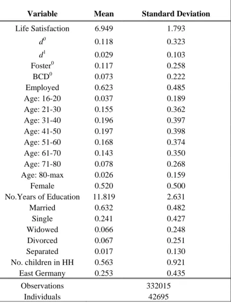
The descriptive statistics of our main sample appear in Table 1 and Figure 1. Our 332,000 observations correspond to almost 42,700 subjects, who are thus observed on average almost 8 years each. The majority of the sample is of working age and is either married (63%) or single (21%). Approximately 62% of the sample is employed at the moment of the survey. Around 12% of observations correspond to respondents whose equivalent income was below 60% of the yearly median income that year: these are the observations corresponding to the poor in our empirical analysis. The average value of our dependent variable, life satisfaction, is close to seven on the zero to ten scale, indicating that there are no striking ceiling or floor effects on average. Life satisfaction is strongly correlated with age, showing the typical U-shape followed by a subsequent drop for the over 65s. It is difficult in Figure 1 to disentangle cohort from age effects; however, our regression analysis will control for individual fixed-effects.
The distribution of poverty by age and gender does not exactly mirror that of life satisfaction. Poverty prevalence is completely U-shaped in age. This is as expected, as earnings tend to peak in the 50s and retirement is typically associated with sharply lower real incomes. However, Figure 1 does suggest that life satisfaction and poverty are related. This is confirmed by the data. Well-being scores of zero to two are reported by
2% of the sample, 27% of whom are in poverty; the analogous figures for well-being scores of eight to ten are 40% and 9% respectively.
Throughout the paper, in order to make full use of the panel nature of our data, and in line with most of the literature on well-being, we use fixed-effects estimation. This allows us to control for otherwise unobserved individual characteristics and any potentially different use of the underlying satisfaction scale across individuals. The general model then takes the form:
[4]
where Cit is the set of time-varying individual covariates and PIit is a series of poverty
indices at the individual level. Depending on the question addressed, both the sample and the form of the PIs will change. With the fixed effect in [4], the coefficients are identified off of within-subject variations. We use “within” fixed-effect linear regressions.
We first establish the relationship between both the incidence and intensity of contemporaneous poverty and life satisfaction: these turn out, unsurprisingly, to be negative. We then introduce time explicitly, and consider the question of adaptation (within a spell) to poverty: Do people “get used” to poverty in the same way that the literature suggests they may adapt to higher income or to marriage? Third, we ask whether poverty has a scarring effect on well-being, that is if the life satisfaction of those who are currently out of poverty is lower if they were poor in the past. Last, we consider the role of persistence, whereby the order of poverty spells matters: For a given number of poverty spells, is satisfaction lower when the spells are concatenated?
5. Results
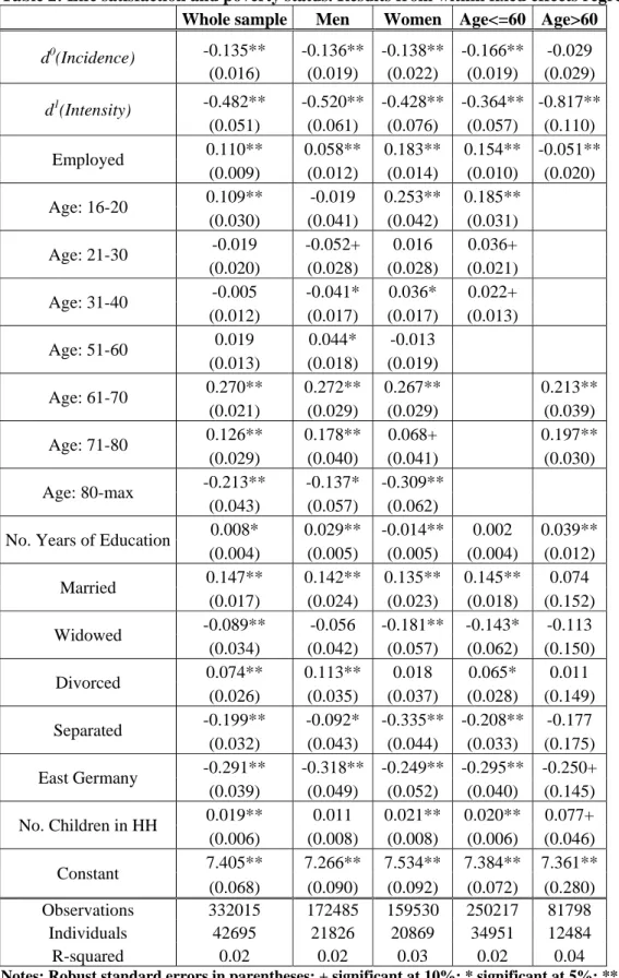
5.1 Current poverty incidence and intensityWe start with the simplest question: the effect of contemporaneous poverty on subjective well-being. Table 2 shows the results from fixed-effect regressions of life satisfaction, in which the estimates refer to within-subject variation.
The regressions include various control variables, which attract the expected coefficients: life satisfaction is U-shaped in age, at least up until age 80. The U-shape
seems sharper for women than for men. Education attracts a positive significant but small coefficient in the overall sample, although it is worth remembering that many individuals will not change their years of education over time. Those who marry are more satisfied, while widowhood and separation are associated with lower life satisfaction, especially for women. The divorced are estimated to be more satisfied in this fixed-effects regression, which is consistent with a rise in well-being compared to a failing marriage. This positive effect is found for male and younger respondents. With respect to labor-force status, we find a positive estimated coefficient, as expected, for employment.
More novel, and central to our research question, are the coefficients on the various poverty measures. At the top of Table 2, both the incidence (d0) and intensity (d1) of poverty are significantly negatively correlated with life satisfaction. This is true also within each subgroup. The estimated effect of poverty in Table 2 is large in size. An individual who lives in a household that is just below the poverty line (so that d0=1 and d1 is almost zero) has a life satisfaction score that is 0.135 points lower than an identical person who is not poor; this effect is of the same magnitude as the happiness boost from marriage. An individual who lives in a household with an income that is half of the poverty line (so that d0=1 and d1, the normalized distance from the poverty line, is 0.5) has a life satisfaction score that is 0.135 + 0.5*0.482 = 0.376 points lower than an identical person who is not poor. This figure is about twice as large as the drop in satisfaction following separation.
5.2 Adaptation to poverty?
Finding that the poor are, on average, less satisfied with their lives than the rich is consistent with much existing work which has underlined a positive correlation between own income and well-being. We can make a more novel contribution by introducing time and asking whether individuals adapt to poverty. Finding that the poor are less satisfied than the rich on average tells us nothing about the time profile of well-being within a poverty spell: this could be decreasing, drop down on entry into poverty and then stay at the same lower level (like a step function), or exhibit partial or even total adaptation. While the existing literature suggests that the well-being profile within an unemployment
spell is a step function, whereas that for marriage exhibits complete adaptation, there is no work on well-being adaptation to poverty.
The sample here is restricted to individuals for whom we observe the first entry into poverty while in the panel, and it is only this first spell that is taken into consideration. We thus compare the life satisfaction of the same individual pre-poverty and during their first observed poverty spell. This is the same method applied to unemployment, marriage, divorce, widowhood and children in SOEP data by Clark et al. (2008a).
We investigate adaptation by splitting up the currently poor into groups according to how long ago they entered poverty. As such, we effectively cut up the d0 dummy from Table 2 into eleven new dummy variables which describe poverty of different durations: these indicate, for the currently poor, whether the individual entered poverty within the past year, 1-2 years ago, and so on up to 10 or more years ago. If the individual adapts, then the coefficients on these dummies should become progressively smaller, since having entered poverty longer ago has a more muted effect on life satisfaction than having become poor more recently.
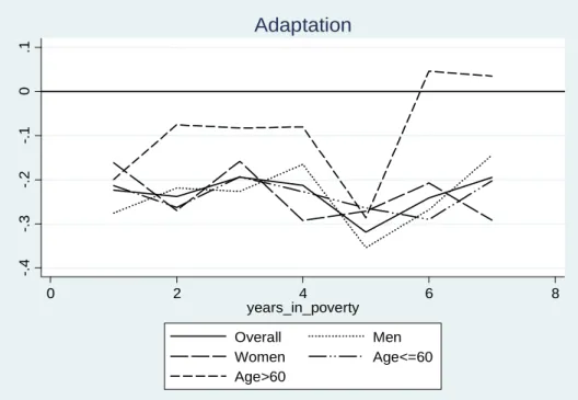
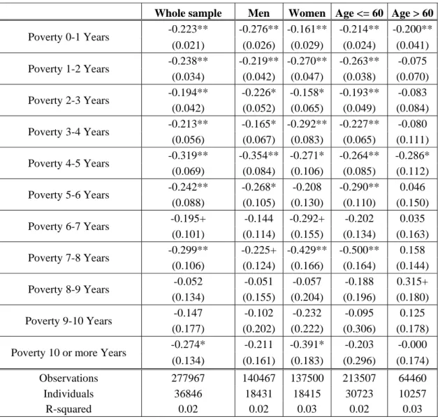
Table 3 shows the results of this analysis. The estimated coefficients there, the first seven which are also plotted for ease of comparison in Figure 2, show that poverty is associated with significantly lower well-being whatever its duration. The estimated coefficients are mostly significant and float around the -0.2 mark. Those on poverty duration of 8-9 years and 9-10 years are also negative but are insignificant. This likely reflects small cell sizes, as that on poverty of 10+ years duration becomes significantly negative again. The estimated coefficients on poverty of different durations in Table 3 are typically not significantly different from each other in the whole sample results in column 1. In general we here have no strong evidence of adaptation to poverty: poverty starts off bad and pretty much stays bad.
The analysis by subgroups reveals no striking differences by gender. However, there is some evidence of adaptation for individuals aged over 60, a finding to which we shall return below.
5.3 Scarring
We now ask whether past poverty has a scarring effect on the well-being of those who are currently not poor. To do so we include a dummy indicating whether an individual has experienced poverty in the past. Since subjects observed for shorter periods do not provide evidence for the medium/long run patterns we are interested in, we only consider those who are observed for at least ten years (although any time restriction we introduce does not particularly affect the qualitative results). This approach might be associated with some bias if individuals leave the survey because they have become poor. However, this is not the case in our panel: poverty incidence is the same for both the excluded and included samples.
The results appear in Table 4. Past poverty experience reduces the life satisfaction of the currently non-poor: poverty is not then ephemeral but has well-being effects that extend beyond the poverty spell. The overall coefficient in column 1 of Table 4 seems to be driven mainly by women and those aged 60 and under. The experience of past poverty has no significant effect for older respondents. This is reminiscent of the result above on adaptation for the over-60s above. The elderly to a certain extent seem to live more day-to-day, by adapting more to circumstances and making the best out of what is currently available.
5.4 Chronic and persistent poverty
Our last question refers to the impact of the cumulated experience of poverty on individual well-being. In this context, we not only consider the past number of years spent in poverty (i.e. chronic poverty), but also ask whether a given number of poverty years reduce well-being more if they are consecutive (which refers to the persistence of poverty).
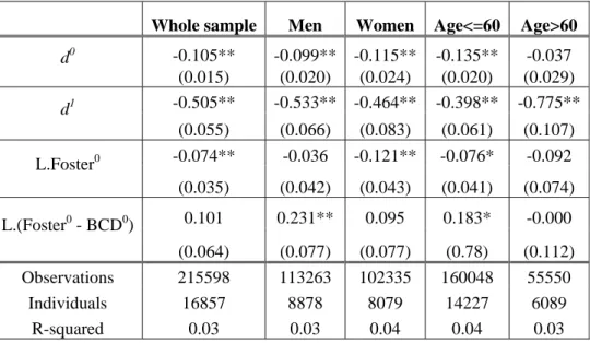
Our last regression thus includes both lagged average past cumulative poverty, given by the Foster index (measuring chronicity, equation [3]), and the normalized Bossert et al. index (measuring persistence, BCD in equation [2]), both calculated over all of the past years, excluding the present. The results presented here refer to the incidence of poverty for both indices (L.Foster0 and L.BCD0, where L stands for "lagged"), as the results are arguably simpler to interpret (although very similar results
pertain if we instead use L.Foster1 and L.BCD1). As equation [2] shows, the BCD persistence index mechanically includes chronicity. In order to disentangle the two, our regressions introduce both L.Foster0 and the difference L.(Foster0 - BCD0) as explanatory variables. This second term then picks up persistence conditional on any effect of chronic poverty. If past poverty persistence reduces current life satisfaction, we expect a positive estimated coefficient on this difference variable.
The results in Table 5 clearly show that the chronicity of poverty, as measured by the Foster index, matters. Chronic poverty attracts a negative coefficient in all of the columns, although the statistical significance varies. Male life satisfaction is not significantly correlated with the cumulative number of years spent in poverty, although as we will see below, men are significantly affected by poverty persistence.
The sign on L.(Foster0 - BCD0) is always positive, as expected. The sequence of a given number of poverty years thus matters, with years that are more consecutive being worse: a succession of shorter exposures in the past has a less negative effect on current well-being than one longer exposure. In the overall sample, the associated coefficient is negative but just insignificant at the ten per cent level. In the sub-regressions, poverty persistence is not significant for women and the elderly, but does matter for men and those aged up to 60. For women then the chronic dimension of poverty counts more than its persistence, while for men it is the other way round. In both cases, however, previous poverty clear affects current well-being.
It is worth underlining that this combination of the indices is asking a lot of the data, as we here identify off of the separate movements in both past poverty incidence (L.Foster0) and persistence (L.BCD0) for the same individual over different years of the SOEP. A version of Table 5 which includes only L.Foster0 or only L.BCD0 yields consistent results, with these always being negatively and significantly correlated with well-being, except for the elderly.
5.5 Do the results depend on the choice of the poverty line?
One concern with the above analysis is the choice of the “right” poverty line. In line with EU practice we consider a relative poverty line given by 60% of the median of the distribution of equivalent income. Although this is a very common assumption, it can
easily be argued that this line is too high or too low: especially as we are here interested in individuals feeling, rather than objectively being, poor. A poverty line that is too high will “dilute” poverty’s impact, by defining as poor some individuals who do not see themselves as such (and, consequently, may not report lower well-being); a line that is too low conversely assigns some people who are poor (and unhappy) to the non-poor group.
As it is difficult to be sure a priori which definition is the best, we re-ran our analyses with different poverty lines. Specifically, we set the poverty line equal to a changing percentage (40%, 50%, 70% and 80%) of the median income. These results are available on request. The negative and significant effect of contemporaneous poverty (incidence and intensity) on life satisfaction pertain in all cases. The past continues to count significantly, except at the extreme values. Specifically, with a 40% poverty line we lose significance on our BCD variable picking up persistence. In a sense this is understandable, as lower poverty lines progressively eliminate poverty spells, meaning we end up with less variance (especially within individual) in our data. With an 80% poverty line, neither of the past poverty measures (L.Foster0 and L.BCD0) are significant in the overall sample, although they continue to occasionally be so in the sub-samples. A high poverty line does seem to dilute the effect of poverty on well-being, especially where the past is concerned. Last, the adaptation profiles, as in Figure 2, are found for all values of the poverty line.
6. Conclusion
We have here used SOEP data to analyze the effects of poverty on individual well-being, and show that both the incidence and intensity of poverty reduce life satisfaction. Our main results relate to the effect of time. We first show that the negative effects of poverty are not ephemeral: there is no evidence that individuals adapt to poverty, and past poverty scars current well-being. In addition, individuals seem to have a preference for income stability, in that persistent poverty is less harmful than the same number of years of low income experienced with movements in and out of poverty. These effects differ to an extent by population subgroups.
We believe that these results are important in three ways. First, they represent new information on the relationship between poverty and subjective well-being explicitly taking the past into account. We have shown that both current and past poverty matter, even in a rich country. Second, we have provided a bridge between theory and empirics, by showing that the most recent literature on poverty indices can be applied to well-known panel data to see which dimensions of poverty are the most salient. Future research may well consider taking a similar line with the vast number of different indices which are now available in the theoretical literature. Third, at a broader level, they show that researchers and policy-makers should continue to be concerned about income distribution and poverty: individuals towards the bottom of the distribution have not adapted to their situation, and past poverty (especially when persistent) reduces current well-being. The candidate happy slaves in the SOEP turn out to be not so happy after all.
References
Alesina, A. and N. Fuchs-Schündeln, (2005), “Good Bye Lenin (or not?): The Effect of Communism on People’s Preferences,” NBER Working Paper No.11700.
Behrman, J., A. Foster, M. Rosenzweig and P. Vashishtha, (1999), “Women's Schooling, Home Teaching, and Economic Growth,” Journal of Political Economy, 107, 682–714. Blanchflower, D.G. and A.J. Oswald, (2004), “Well-Being over Time in Britain and the USA,” Journal of Public Economics, 88, 1359–1386.
Bossert, W., C. D’Ambrosio and S.R. Chakravarty, (2012), “Poverty and Time,” Journal of Economic Inequality, 10, 145–162.
Blake, H. (2012), “How Do Recession and Unemployment Impact Children in the Long Term?,” PSE, mimeo.
Burchardt, T., (2005), “Are One Man’s Rags Another Man’s Riches? Identifying Adaptive Expectations Using Panel Data,” Social Indicators Research, 74, 57–102.
Cappellari, L. and S.P. Jenkins, (2004), “Modelling low income transitions,” Journal of Applied Econometrics, 19, 593–610.
Christiaensen, L. and T. Shorrocks, (2012), “Measuring Poverty Over Time,” Journal of Economic Inequality, 10, 137–143.
Clark, A.E., E. Diener, Y. Georgellis and R.E. Lucas, (2008a), “Lags and Leads in Life Satisfaction: a Test of the Baseline Hypothesis,” Economic Journal, 118, F222–F243. Clark, A.E., P. Frijters and M. Shields, (2008b), “Relative Income, Happiness and Utility: An Explanation for the Easterlin Paradox and Other Puzzles,” Journal of Economic Literature, 46, 95-144.
Clark, A.E. and Y. Georgellis, (2013), “Back to Baseline in Britain: Adaptation in the BHPS,” Economica, forthcoming.
Clark, A.E., Y. Georgellis and P. Sanfey, (2001), “Scarring: the Psychological Impact of Past Unemployment,” Economica, 68, 221–241.
Clark, D.A., (2009), “Adaptation, Poverty and Well-Being: Some Issues and Observations with Special Reference to the Capability Approach and Development Studies,” Journal of Human Development and Capabilities, 10, 21–42.
Diener, E. and R. Biswas-Diener, (2002), “Will Money Increase Subjective Well-Being? A Literature Review and Guide to Needed Research,” Social Indicators Research, 57, 119–169.
Diener, E., W. Ng, J. Harter and R. Arora, (2010), “Wealth and Happiness Across the World: Material Prosperity Predicts Life Evaluation, Whereas Psychosocial Prosperity Predicts Positive Feeling,” Journal of Personality and Social Psychology, 99, 52–61. Di Tella, R., J. Haisken-De New and R. MacCulloch, (2010), “Happiness Adaptation to Income and to Status in an Individual Panel,” Journal of Economic Behavior & Organization, 76, 834–852.
Di Tella, R. and R. MacCulloch, (2006), “Some Uses of Happiness Data in Economics,” Journal of Economic Perspectives, 20, 25–46.
Di Tella, R. and R. MacCulloch, (2010), “Happiness Adaptation to Income Beyond "Basic Needs",” in: E. Diener, J. Helliwell and D. Kahneman, eds., International Differences in Well-Being. Oxford, Oxford University Press, 217–246.
Easterlin, R.A., (1974), “Does Economic Growth Improve the Human Lot?,” in: P.A. David and M.W. Reder, eds., Nations and households in economic growth: Essays in honor of Moses Abramovitz, New York, Academic Press, 89–125.
Easterlin, R.A., (1995), “Will raising the incomes of all increase the happiness of all?,” Journal of Economic Behavior and Organization, 27, 35–48.
Fernández, R., A. Fogli and C. Olivetti, (2004), “Mothers and Sons: Preference Formation and Female Labor Force Dynamics,” Quarterly Journal of Economics, 119, 1249–1299.
Foster, J.E., (2009), “A Class of Chronic Poverty Measures,” in: T. Addison, D. Hulme and R. Kanbur, eds., Poverty dynamics: interdisciplinary perspectives, Oxford, Oxford University Press, 59–76.
Foster, J., J, Greer and E. Thorbecke, (1984), “A Class of Decomposable Poverty Measures,” Econometrica, 81, 761–766.
Frey, B.S. and A. Stutzer, (2002), Happiness and Economics: How the Economy and Institutions Affect Human Well-Being, Princeton, Princeton University Press.
Frijters, P., D. Johnston and M. Shields, (2011a), “Happiness Dynamics with Quarterly Life Event Data,” Scandinavian Journal of Economics, 113, 190–211.
Frijters, P., D. Johnston and M. Shields, (2011b), “Destined for (Un)Happiness: Does Childhood Predict Adult Life Satisfaction?,” IZA, Discussion Paper No.5819.
Giuliano, P. and A. Spilimbergo, (2009), “Growing Up in a Recession: Beliefs and the Macroeconomy,” NBER Working Paper No.15321.
Hotz, V., F. Kydland and G. Sedlacek, (1988), “Intertemporal Preferences and Labor Supply,” Econometrica, 56, 335–360.
Kahneman, D. and A. Tversky, (1979), “Prospect Theory: An Analysis of Decision Under Risk,” Econometrica, 47, 263–291.
Kaustia, M. and S. Knüpfer, (2008), “Do Investors Overweight Personal Experience? Evidence from IPO Subscriptions,” Journal of Finance, 63, 2679–2702.
Knabe, A. and S. Rätzel, (2011), “Scarring or Scaring? The Psychological Impact of Past Unemployment and Future Unemployment Risk,” Economica, 78, 283–293.
Lange, T., (2013), “Scarred from the Past or Afraid of the Future? Unemployment and Job Satisfaction across European Labour Markets,” International Journal of Human Resource Management, 24, 1096-1112.
Layard, R., A.E. Clark, F. Cornaglia, N. Powdthavee and J. Vernoit, (2013), “What Predicts a Successful Life? A Life-Course Model of Wellbeing,” LSE, mimeo.
Malmendier, U. and S. Nagel, (2011), “Depression Babies: do Macroeconomic Experiences Affect Risk-taking?” Quarterly Journal of Economics, 126, 373–416.
Nowok, B., M. Van Ham, A. Findlay and V. Gayle, (2013), “Does Migration Make You Happy? A Longitudinal Study of Internal Migration and Subjective Well-Being,” Environment and Planning A, forthcoming.
Oswald, A.J. and N. Powdthavee, (2008), “Does Happiness Adapt? A Longitudinal Study of Disability with Implications for Economists and Judges,” Journal of Public Economics, 92, 1061–1077.
Rosenzweig, M. and K. Wolpin, (1994), “Inequality among Young Adult Siblings, Public Assistance Programs, and Intergenerational Living Arrangements,” Journal of Human Resources, 29, 1101–1125.
Ruhm, C.J. (1991), “Are Workers Permanently Scarred by Job Displacements?,” American Economic Review, 81, 319–24.
Sen, A.K., (1990), “Development as Capability Expansion,” in K. Griffin and J. Knight, eds., Human Development and the International Development Strategy for the 1990s, London, Macmillan, 41–58.
Senik, C., (1995), “Income Distribution and Well-Being: What Can we Learn from Subjective Data?,” Journal of Economic Surveys, 19, 43–63.
Voigtländer, M., (2011), “Why is the German Homeownership Rate so Low?,” Housing Studies, 24, 355–372.
Wagner, G., J. Frick and J. Schupp, (2007), “The German Socio-Economic Panel Study (SOEP) - Scope, Evolution and Enhancements,” Schmollers Jahrbuch, 127, 139-169. World Bank, (2005), “Introduction to Poverty Analysis,” the World Bank Institute, Washington, downloadable at:
Figure 1: Poverty and Well-being by gender and age.
Figure 2: Adaptation to poverty. The first seven coefficients from panel regressions for individuals entering their first observed poverty spell .
6. 7 7. 2 5 Li fe S a ti s fac ti o n 20 40 60 80 Age of Individual Women Men
Well-being by age and sex
.0 5 .2 5 P rev a len c e 20 40 60 80 Age of Individual Women Men
Poverty prevalence by age and sex
-.4 -. 3 -. 2 -. 1 0 .1 0 2 4 6 8 years_in_poverty Overall Men Women Age<=60 Age>60 Adaptation
Table 1: Descriptive Statistics in the Main Sample.
Variable Mean Standard Deviation
Life Satisfaction 6.949 1.793 d0 0.118 0.323 d1 0.029 0.103 Foster0 0.117 0.258 BCD0 0.073 0.222 Employed 0.623 0.485 Age: 16-20 0.037 0.189 Age: 21-30 0.155 0.362 Age: 31-40 0.196 0.397 Age: 41-50 0.197 0.398 Age: 51-60 0.168 0.374 Age: 61-70 0.143 0.350 Age: 71-80 0.078 0.268 Age: 80-max 0.026 0.159 Female 0.520 0.500 No.Years of Education 11.819 2.631 Married 0.632 0.482 Single 0.241 0.427 Widowed 0.066 0.248 Divorced 0.067 0.251 Separated 0.017 0.130 No. children in HH 0.563 0.921 East Germany 0.253 0.435 Observations 332015 Individuals 42695
Table 2: Life satisfaction and poverty status. Results from within fixed effects regressions. Whole sample Men Women Age<=60 Age>60
d0(Incidence) -0.135** -0.136** -0.138** -0.166** -0.029 (0.016) (0.019) (0.022) (0.019) (0.029) d1(Intensity) -0.482** -0.520** -0.428** -0.364** -0.817** (0.051) (0.061) (0.076) (0.057) (0.110) Employed 0.110** 0.058** 0.183** 0.154** -0.051** (0.009) (0.012) (0.014) (0.010) (0.020) Age: 16-20 0.109** -0.019 0.253** 0.185** (0.030) (0.041) (0.042) (0.031) Age: 21-30 -0.019 -0.052+ 0.016 0.036+ (0.020) (0.028) (0.028) (0.021) Age: 31-40 -0.005 -0.041* 0.036* 0.022+ (0.012) (0.017) (0.017) (0.013) Age: 51-60 0.019 0.044* -0.013 (0.013) (0.018) (0.019) Age: 61-70 0.270** 0.272** 0.267** 0.213** (0.021) (0.029) (0.029) (0.039) Age: 71-80 0.126** 0.178** 0.068+ 0.197** (0.029) (0.040) (0.041) (0.030) Age: 80-max -0.213** -0.137* -0.309** (0.043) (0.057) (0.062)
No. Years of Education 0.008* 0.029** -0.014** 0.002 0.039** (0.004) (0.005) (0.005) (0.004) (0.012) Married 0.147** 0.142** 0.135** 0.145** 0.074 (0.017) (0.024) (0.023) (0.018) (0.152) Widowed -0.089** -0.056 -0.181** -0.143* -0.113 (0.034) (0.042) (0.057) (0.062) (0.150) Divorced 0.074** 0.113** 0.018 0.065* 0.011 (0.026) (0.035) (0.037) (0.028) (0.149) Separated -0.199** -0.092* -0.335** -0.208** -0.177 (0.032) (0.043) (0.044) (0.033) (0.175) East Germany -0.291** -0.318** -0.249** -0.295** -0.250+ (0.039) (0.049) (0.052) (0.040) (0.145) No. Children in HH 0.019** 0.011 0.021** 0.020** 0.077+ (0.006) (0.008) (0.008) (0.006) (0.046) Constant 7.405** 7.266** 7.534** 7.384** 7.361** (0.068) (0.090) (0.092) (0.072) (0.280) Observations 332015 172485 159530 250217 81798 Individuals 42695 21826 20869 34951 12484 R-squared 0.02 0.02 0.03 0.02 0.04
Notes: Robust standard errors in parentheses; + significant at 10%; * significant at 5%; ** significant at 1%.
Table 3: Adaptation to poverty. Results from within fixed effects regressions on individuals who entered their first poverty spell while in the panel.
Whole sample Men Women Age <= 60 Age > 60 Poverty 0-1 Years -0.223** -0.276** -0.161** -0.214** -0.200** (0.021) (0.026) (0.029) (0.024) (0.041) Poverty 1-2 Years -0.238** -0.219** -0.270** -0.263** -0.075 (0.034) (0.042) (0.047) (0.038) (0.070) Poverty 2-3 Years -0.194** -0.226* -0.158* -0.193** -0.083 (0.042) (0.052) (0.065) (0.049) (0.084) Poverty 3-4 Years -0.213** -0.165* -0.292** -0.227** -0.080 (0.056) (0.067) (0.083) (0.065) (0.111) Poverty 4-5 Years -0.319** -0.354** -0.271* -0.264** -0.286* (0.069) (0.084) (0.106) (0.085) (0.112) Poverty 5-6 Years -0.242** -0.268* -0.208 -0.290** 0.046 (0.088) (0.105) (0.130) (0.110) (0.150) Poverty 6-7 Years -0.195+ -0.144 -0.292+ -0.202 0.035 (0.101) (0.114) (0.155) (0.134) (0.163) Poverty 7-8 Years -0.299** -0.225+ -0.429** -0.500** 0.158 (0.106) (0.124) (0.166) (0.164) (0.144) Poverty 8-9 Years -0.052 -0.051 -0.057 -0.188 0.315+ (0.134) (0.155) (0.204) (0.196) (0.180) Poverty 9-10 Years -0.147 -0.102 -0.232 -0.095 0.125 (0.177) (0.202) (0.222) (0.306) (0.178)
Poverty 10 or more Years -0.274* -0.211 -0.391* -0.203 -0.000 (0.134) (0.161) (0.183) (0.296) (0.174)
Observations 277967 140467 137500 213507 64460
Individuals 36846 18431 18415 30723 10257
R-squared 0.02 0.02 0.03 0.02 0.03
Notes: Robust standard errors in parentheses; + significant at 10%; * significant at 5%; ** significant at 1%; the regressions include all of the other control variables in Table 2.
Table 4: The scarring effect of poverty on life satisfaction. Results from fixed effects regressions for individuals observed for at least 10 years.
Whole sample Men Women Age <= 60 Age > 60
Past poverty -0.053** -0.041+ -0.077** -0.067** -0.073 (0.019) (0.027) (0.027) (0.023) (0.046) Observations 206207 106069 100138 157121 49080
Individuals 16706 8707 8030 14309 5787
R-squared 0.02 0.02 0.02 0.03 0.03
Notes: Standard errors in parentheses; + significant at 10%; * significant at 5%; ** significant at 1%; the regressions include all of the other control variables in Table 2.
Table 5: Chronic poverty and persistence. Results from fixed effects regressions for individuals observed for at least 10 years.
Whole sample Men Women Age<=60 Age>60 d0 -0.105** -0.099** -0.115** -0.135** -0.037 (0.015) (0.020) (0.024) (0.020) (0.029) d1 -0.505** -0.533** -0.464** -0.398** -0.775** (0.055) (0.066) (0.083) (0.061) (0.107) L.Foster0 -0.074** -0.036 -0.121** -0.076* -0.092 (0.035) (0.042) (0.043) (0.041) (0.074) L.(Foster0 - BCD0) 0.101 0.231** 0.095 0.183* -0.000 (0.064) (0.077) (0.077) (0.78) (0.112) Observations 215598 113263 102335 160048 55550 Individuals 16857 8878 8079 14227 6089 R-squared 0.03 0.03 0.04 0.04 0.03
Note: Standard errors in parentheses; + significant at 10%; * significant at 5%; ** significant at 1%; the regressions include all of the other control variables in Table 2.