A framework to understand the transient climate response to emissions

HAL Id: hal-01587293

https://hal.archives-ouvertes.fr/hal-01587293

Submitted on 28 May 2019

HAL is a multi-disciplinary open access

archive for the deposit and dissemination of

sci-entific research documents, whether they are

pub-lished or not. The documents may come from

teaching and research institutions in France or

abroad, or from public or private research centers.

L’archive ouverte pluridisciplinaire HAL, est

destinée au dépôt et à la diffusion de documents

scientifiques de niveau recherche, publiés ou non,

émanant des établissements d’enseignement et de

recherche français ou étrangers, des laboratoires

publics ou privés.

response to emissions

Richard G Williams, Philip Goodwin, Vassil M Roussenov, Laurent Bopp

To cite this version:

Richard G Williams, Philip Goodwin, Vassil M Roussenov, Laurent Bopp. A framework to understand

the transient climate response to emissions. Environmental Research Letters, IOP Publishing, 2016,

11 (1), pp.015003. �10.1088/1748-9326/11/1/015003�. �hal-01587293�

LETTER • OPEN ACCESS

A framework to understand the transient climate

response to emissions

To cite this article: Richard G Williams et al 2016 Environ. Res. Lett. 11 015003

View the article online for updates and enhancements.

Related content

Examination of a climate stabilization pathway via zero-emissions using Earth system models

Daisuke Nohara, J Tsutsui, S Watanabe et al.

-Sensitivity of carbon budgets to permafrost carbon feedbacks and non-CO2 forcings

Andrew H MacDougall, Kirsten Zickfeld, Reto Knutti et al.

-Extending the relationship between global warming and cumulative carbon emissions to multi-millennial timescales

Thomas L Frölicher and David J Paynter

-Recent citations

Reconciling Atmospheric and Oceanic Views of the Transient Climate Response to Emissions

Anna Katavouta et al

-Quantifying Land and People Exposed to Sea-Level Rise with No Mitigation and 1.5°C and 2.0°C Rise in Global Temperatures to Year 2300

S. Brown et al

-Adjusting Mitigation Pathways to Stabilize Climate at 1.5°C and 2.0°C Rise in Global Temperatures to Year 2300

Philip Goodwin et al

LETTER

A framework to understand the transient climate response to

emissions

Richard G Williams1

, Philip Goodwin2

, Vassil M Roussenov1

and Laurent Bopp3

1 _{Department of Earth, Ocean & Ecological Sciences, School of Environmental Sciences, Liverpool University, Liverpool, UK} 2 _{School of Ocean and Earth Sciences, Southampton University, Southampton, UK}

3 _{Laboratoire des Sciences du Climat et de l’Environment, Institut Pierre-Simon Laplace, CNRS/CEA/UVSQ, CEA Saclay, Gif-sur-Yvette,}

France

E-mail:ric@liv.ac.uk

Keywords: transient climate response to emissions, climate change, cumulative carbon emissions, radiative forcing from CO2, ocean heat

and carbon drawdown

Abstract

Global surface warming projections have been empirically connected to carbon emissions via a climate

index defined as the transient climate response to emissions (TCRE), revealing that surface warming is

nearly proportional to carbon emissions. Here, we provide a theoretical framework to understand the

TCRE including the effects of all radiative forcing in terms of the product of three terms: the

dependence of surface warming on radiative forcing, the fractional radiative forcing contribution from

atmospheric CO

and the dependence of radiative forcing from atmospheric CO

on cumulative

carbon emissions. This framework is used to interpret the climate response over the next century for

two Earth System Models of differing complexity, both containing a representation of the carbon cycle:

an Earth System Model of Intermediate Complexity, configured as an idealised coupled atmosphere

and ocean, and an Earth System Model, based on an atmosphere–ocean general circulation model and

including non-CO

radiative forcing and a land carbon cycle. Both Earth System Models simulate only

a slight decrease in the TCRE over 2005–2100. This limited change in the TCRE is due to the ocean and

terrestrial system acting to sequester both heat and carbon: carbon uptake acts to decrease the

dependence of radiative forcing from CO

on carbon emissions, which is partly compensated by

changes in ocean heat uptake acting to increase the dependence of surface warming on radiative

forcing. On decadal timescales, there are larger changes in the TCRE due to changes in ocean heat

uptake and changes in non-CO

radiative forcing, as represented by decadal changes in the

dependences of surface warming on radiative forcing and the fractional radiative forcing contribution

from atmospheric CO

. Our framework may be used to interpret the response of different climate

models and used to provide traceability between climate models of differing complexity.

1. Introduction

Surface global warming is empirically found in climate models to be nearly linearly dependent on the cumulative amount of carbon emitted to the climate system. This climate relationship wasfirst set out in terms of how the peak warming of a range of climate models depends on the cumulative amount of carbon emitted(Allen et al2009) and how the global warming

in climate model projections is proportional to cumulative carbon emissions (Matthews et al2009,

Zickfeld et al2009). Both these responses are largely

independent of emission pathway, but the amplitude of the climate response varies with individual climate models. The proportionality of global surface warming to cumulative carbon emissions is used to define the transient climate response to emissions(TCRE, in K per 1000 PgC) (Collins et al2013, Gillet et al2013).

The TCRE is found to be approximately independent of time and emission scenario; for example, the proportionality of the surface warming to cumulative carbon emissions is depicted here infigure1(a) by the

OPEN ACCESS

RECEIVED 25 September 2015 REVISED 14 December 2015 ACCEPTED FOR PUBLICATION 16 December 2015 PUBLISHED 21 January 2016

Original content from this work may be used under the terms of theCreative Commons Attribution 3.0 licence.

Any further distribution of this work must maintain attribution to the author(s) and the title of the work, journal citation and DOI.

slope of the warming response versus cumulative emissions for two Earth System Models of differing complexity for a range of emission scenarios.

Recently Goodwin et al(2015) provided a single

equation to connect surface warming to carbon emis-sions, drawing upon theoretical relations for the global heat balance and carbon inventories for the climate system. Based on this equation, the near constancy in the TCRE is explained in terms of partly compensating effects of the ocean heat and carbon uptake, extending heuristic arguments of Solomon et al(2009), where the

cooling effect of ocean uptake of atmospheric CO2is

accompanied by a partly-compensating surface warm-ing effect by declinwarm-ing ocean heat uptake. This time-dependent relationship for the TCRE asymptotes to a long-term equilibrium response, defined by the climate and carbon parameters for the climate system (Williams et al2012).

In this study, we develop a framework to interpret how the TCRE is controlled, the dependence of surface warming on cumulative carbon emissions, which is separated into the product of the dependence of

surface warming on the radiative forcing from atmo-spheric CO2and the dependence of the radiative

for-cing from atmospheric CO2on carbon emissions. This

TCRE definition is also extended to include the effect of other non-CO2radiative forcing via a

non-dimen-sional term, the fractional radiative forcing contrib-ution from CO2. The TCRE framework is then

combined with our theoretical relations for the global heat balance and buffered carbon inventories (Good-win et al2015). Our TCRE framework is illustrated

using diagnostics of an Earth System Model of Inter-mediate Complexity(GENIE) and an Earth System Model(IPSL-CM5A-LR). GENIE is configured as an idealised atmosphere–ocean model and only includes radiative forcing from atmospheric CO2, while

IPSL-CM5A-LR additionally includes non-CO2 radiative

forcing and a representation of the land carbon cycle. Both models are integrated from a pre-industrial state and their climate response diagnosed in terms of our framework for their projections from 2005 to 2100.

The paper is set out as follows: the theoretical fra-mework isfirst presented to understand the TCRE and Figure 1.(a) Diagnostics of surface warming, ΔT (K), versus cumulative carbon emissions, ΔI (PgC), for different RCP scenarios for two different Earth System Models integrated from 2000 to 2100(dots every 50 years): an Earth System Model of Intermediate Complexity(GENIE) (left panel) and the Earth System Model IPSL-CM5A-LR (right panel). The slope of the lines represent the transient climate response to emissions_{(TCRE). (b) A schematic view of how cumulative carbon emissions are linked to surface} warming via the TCRE(black arrow). However, we advocate that the TCRE can be viewed in terms of the dependence of surface warming on radiative forcing(red arrow), the fractional radiative forcing contribution from atmospheric CO2(grey arrow) and the

our extension to include the non-CO2radiative

for-cing contribution (section 2); the Earth System

Model of Intermediate Complexity and Earth System Model are diagnosed in terms of changes in the TCRE and its dependences (section 3); the mechanistic

implications from our framework are then discussed (section 4) and finally conclusions are provided

(section5).

2. Theory

A new framework is set out to understand the dependence of the TCRE. This framework draws upon our prior studies for the time-dependent climate response (Goodwin et al 2015) and the long-term

equilibrium climate response(Williams et al2012) to

cumulative carbon emissions. 2.1. Theoretical framework

In order to understand our framework, assume that the global-mean surface air temperature(K) at time t,

T t ,( ) is defined by a time-dependent anomaly,

T t ,( )

D relative to the temperature at the pre-indus-trial at time to, T t( )=T t( )o + DT t .( ) The

cumula-tive amount of carbon (PgC) emitted to the atmosphere from all anthropogenic sources at time t is similarly defined, I t( )=I t( )o + DI t ,( ) with I t( )o

taken to be zero. The surface temperature anomaly is then related to the cumulative amount of carbon emitted since the pre-industrial via the transient climate response to cumulative carbon emissions, the TCRE, represented mathematically byDT/DI,

T t T I I t , 1 ( ) ⎜⎛ ⎟ ( ) ( ) ⎝ ⎞ ⎠ D = D D D

where theΔ notation denotes differences relative to the pre-industrial (rather than a small incremental interval). Our aim is now to connect this surface warming definition (1) to the controlling factors for

the TCRE, which are assumed to be the dependence of surface warming on radiative forcing and the depend-ence of radiative forcing on cumulative carbon emissions.

Start by assuming that the radiative forcing (W m−2_{) driving climate change is only from}

atmo-spheric CO2, which is defined by RCO2( ) =t RCO2( )to + DRCO2( )t .Here we choose to express the

TCRE in(1) in terms of the product of the dependence

of surface warming on radiative forcing from atmo-spheric CO2, DT/DRCO2, and the dependence of

radiative forcing on carbon emissions,DRCO2/DI: T I T R R I TCRE . 2 CO CO 2 2 _{( )} ⎛ ⎝ ⎜ ⎞ ⎠ ⎟⎛_⎝⎜ ⎞ ⎠ ⎟ = D D = D D D D

More generally, the radiative forcing driving climate change includes contributions from atmo-spheric CO2and other non-CO2contributions, so that

the change in radiative forcing since the pre-industrial

era is given by DR t( )= DRCO2( )t + DRnonCO2( )t .

The change in non-CO2 radiative forcing,

RnonCO2( )t ,

D includes contributions from aerosols emitted via anthropogenic and volcanic activity (Ottera et al2010, Booth et al2012) and other

non-CO2greenhouse gases, such as methane with a shorter

lifetime than CO2(Pierrehumbert2014).

The definition of the TCRE may be extended to include the effect of all contributions to the radiative forcing, such that

T I T R R I TCREallR ⎜ ⎟⎜ ⎟. ( )3 ⎛ ⎝ ⎞ ⎠ ⎛ ⎝ ⎞ ⎠ = D D = D D D D

While this definition looses the clarity of the origi-nal TCRE definition in (2) in terms of isolating the

cli-mate response to cumulative carbon emissions, this generalisation for TCREall Rin(3) is needed if the

cli-mate response is to be diagnosed from a clicli-mate model including non-CO2 radiative forcing. To extend the

TCRE definition in (3), the surface temperature

change in(1) is written as T t T I I t T R R I I t T R R t a , 4 CO nonCO 2 2 ( ) ( ) ( ) ( ) ( ) ⎜ ⎟ ⎜ ⎟ ⎛ ⎝ ⎞ ⎠ ⎛ ⎝ ⎜ ⎞ ⎠ ⎟ ⎛ ⎝ ⎞ ⎠ D =D D D = D D D D D + D D D

which makes explicit the surface warming from the separate effects of the radiative forcing from CO2

and non-CO2contributions. Exploiting the definition

of DR t( )= DRCO2( )t + DRnonCO2( )t , the surface

warming is then equivalently written as

T t T I I t T R R R R I I t . 4b CO CO 2 2 ( ) ( ) ( ) ( ) ⎜ ⎟ ⎛ ⎝ ⎞ ⎠ ⎛ ⎝ ⎜ ⎞ ⎠ ⎟ ⎛ ⎝ ⎜ ⎞ ⎠ ⎟ D = D D D = D D D D ´ D D D

Accordingly, the definition for the TCRE for all radiative forcing contributions in(3) is then expressed

as T I T R R R R I TCRE . 5 R all CO CO 2 2 ( ) ⎜ ⎟ ⎛ ⎝ ⎞ ⎠ ⎛ ⎝ ⎜ ⎞ ⎠ ⎟⎛_⎝⎜ ⎞_⎠⎟ = D D = D D D D D D

This definition of the TCRE for all radiative for-cing contributions in(5) is made up of the product of

three differential terms: the dependence of surface warming on radiative forcing, DT/DR; the frac-tional radiative contribution from atmospheric CO2, DR/DRCO2; and the dependence of radiative

forcing from atmospheric CO2on carbon emissions,

RCO2 I

D /D (depicted in figure1(b) by red, grey and

blue arrows respectively). This definition of the TCRE for all radiative forcings shares the same dependence of the radiative forcing from CO2 on

cumulative carbon emissions,DRCO2/DI,as

generalised to include the non-CO2radiative forcing

contribution.

Our aim is now to assess the behaviour of the TCRE on centennial timescales using a combination of ocean theory and diagnostics of two Earth System Models, GENIE only including radiative forcing from atmospheric CO2and IPSL-CM5A-LR including CO2

and non-CO2radiative forcing.

Our ocean theory is only appropriate for the dependence of surface warming on radiative forcing,

T R

D /D and the dependence of radiative forcing from atmospheric CO2on carbon emissions, DRCO2/DI.

The diagnostics of the TCRE and TCREall Rusing(2)

and (5) respectively are automatically the same for

GENIE, but differ for IPSL-CM5A-LR. On centennial and millennial timescales, we expect that the climate response is dominated by the effect of carbon emis-sions, so that the TCRE and TCREall Rbecome similar

to each other. However, on shorter timescales, the TCRE and TCREall Rdiffer from each other due to the

effects of other forcing agents, such as aerosols and non-CO2greenhouse gases.

2.2. Applying global heat and buffered carbon integral balances

Our framework defining the TCRE and TCREall Rin

(2) and (5) respectively is now combined with

theor-etical balances for a global heat balance and buffered carbon inventory following Goodwin et al(2015).

The global heat balance for climate change involves an increase in radiative forcing since the pre-industrial,ΔR(t) (W m−2, positive downward) driving a climate response, involving additional outgoing longwave radiation, λΔT(t) (W m−2), from the increase in global-mean surface air temperature plus the net downward heatflux into the climate system, N (t) (W m−2_{) (Gregory et al 2004, Gregory and}

For-ster2008)

R t( ) l T t( ) eN t ,( ) ( )6 D = D +

where λ is the equilibrium climate parameter (W m−2_K−1_{) and N t()e is the scaled net heatflux into}

the climate system. The net heat flux N t() is dominated by the ocean heat uptake, accounting for over 90% of the anthropogenic warming of the climate system(Church et al2011). The net heat flux N t() is

scaled in(6) by a non-dimensional parameter, ε, to

take into account the enhanced effect of ocean heat flux in increasing global-mean surface temperature relative to global-mean radiative forcing (Hansen et al1984, Winton et al2010). This heat balance is

rearranged to provide an expression for the depend-ence of surface warming on radiative forcing

T R N t R t 1 1 ( ) , 7 ( ) ( ) ⎛ ⎝ ⎜ ⎞_⎠⎟ l e ¶ ¶ = - D

where the fractional form,DT/DR,is replaced by a differential form as there is a functional relationship and the effective ocean heatflux is normalised by the radiative forcing, N te ( )/DR t( ).

The buffered carbon inventory connects the loga-rithm of atmospheric CO2to the sum of the

cumula-tive carbon emission, ΔI(t), plus the carbon undersaturation of the ocean, IUsat(t) (PgC), minus the

increase in the terrestrial carbon uptake, ΔIter(t)

(PgC), all divided by the buffered carbon inventory, IB

(PgC) (Goodwin et al2015): t I I t I t I t lnCO 1 , 8 2 B Usat ter ( ) ( ( ) ( ) ( )) ( ) D = D + - D

where CO2is the mixing ratio of atmospheric carbon

dioxide(ppm), IUsat(t) is how much carbon the ocean

needs to take up to reach an equilibrium with the atmosphere and DIter( )t =Iter( )t -Iter( )to is the

change in the residual terrestrial carbon sink since the pre-industrial era and IB is the buffered carbon

inventory for the atmosphere and ocean (Goodwin et al2007). This buffered carbon inventory takes into

account a positive feedback; increasing atmospheric CO2enhances ocean acidity and inhibits the ability of

the ocean to take up more atmospheric CO2leading to

an increasing fraction of the emitted carbon remaining in the atmosphere; thus, (8) expresses how

atmo-spheric CO2increases exponentially with the sum of

the cumulative carbon emission plus the ocean under-saturation and minus the terrestrial uptake.

The global heat balance(6) and buffered carbon

inventory(8) are connected together via the radiative

forcing from atmospheric CO2,DRCO2( )t ,defined by

the logarithm of atmospheric CO2(Myhre et al1998)

RCO2( )t a lnCO2( )t , ( )9 D = D

where the logarithm conveys how there is a saturating effect of increasing atmospheric CO2 on radiative

forcing.

Combing the buffered carbon balance(8) with the

definition for radiative forcing from atmospheric CO2

(9) then provides an expression for the dependence of

radiative forcing from atmospheric CO2 on carbon

emissions(Goodwin et al2015) R I a I I t I t I t I t 1 , 10 CO B Usat ter 2 ( ) ( ) ( ) ( ) ( ) ⎛ ⎝ ⎜ ⎞_⎠⎟ ¶ ¶ = + D -D D

where the effects of the ocean carbon undersaturation and increase in terrestrial carbon store are normalised by the cumulative carbon emission,

IUsat t Iter t I t .

( ( )- D ( ))/D ( ) By combining the differ-ential relations(7) and (10), the TCRE definition for all

radiative forcing contributions in(5) becomes a I N t R t I t I t I t I t R t R t TCRE 1 1 . 11 R all B Usat ter CO2 ( ) ( ) ( ) ( ) ( ) ( ) ( ) ( ) ( ) ⎛ ⎝ ⎜ ⎞ ⎠ ⎟ ⎛ ⎝ ⎜ ⎞ ⎠ ⎟⎛ ⎝ ⎜ ⎞ ⎠ ⎟ l e = -D ´ + D -D D D D

The TCREall Rdepends on the time-independent

factors, a/(lI ,B) multiplied by the non-dimensional

time-dependent terms contained within the three pairs of parentheses: the dependence of surface

warming varying with ocean heat uptake; the depend-ence of radiative forcing from atmospheric CO2

vary-ing with ocean carbon undersaturation; and the fractional dependence of radiative forcing on atmo-spheric CO2. As derived by Goodwin et al(2015), if

there is only radiative forcing from CO2, the TCRE

simplifies to T I a I N t R t I t I t I t I t TCRE 1 1 . 12 B Usat ter ( ) ( ) ( ) ( ) ( ) ( ) ( ) ⎛ ⎝ ⎜ ⎞ ⎠ ⎟ ⎛ ⎝ ⎜ ⎞_⎠⎟ l e = D D = - D ´ + D -D D

2.3. Equilibrium response for the TCRE

For a long-term equilibrium when the radiative forcing is only from atmospheric CO2, the TCRE

asymptotes to a response given by the time-indepen-dent factors a/(λIB) (Williams et al2012)

T I a I . 13 t equilib B ( ) l D D  =

To evaluate the equilibrium response, a(W m−2) is the coefficient for the radiative forcing dependence on atmospheric CO2 (Myhre et al 1998, Forster

et al2013); l(W m−2K−1) is the climate parameter (Gregory et al2004) and equivalently_l-1_{is the}

equili-brium climate sensitivity(Knutti and Hegerl 2008);

and IB(PgC) is the buffered carbon inventory for the

atmosphere and ocean(Goodwin et al2007).

The buffered carbon inventory of the atmosphere and ocean, IB, represents the accessible amount of

carbon in the atmosphere and ocean, and takes into account how the buffering of the ocean carbonate sys-tem inhibits the release of carbon from the ocean to the atmosphere: IBis defined for the pre-industrial era

(Goodwin et al2007) as

IB=IA+V DICsat/B, (14)

where IA is the atmospheric inventory of carbon

(PgC), DICsat is the saturated ocean dissolved

inorganic carbon (gC m−3) and B is the non-dimensional buffer factor, and V is the volume of the ocean(m3) (table1). The buffer factor, B, represents

the enhanced fractional changes in atmospheric CO2, relative to the fractional changes in the

saturated dissolved inorganic carbon DIC ,sat where B=(dCO CO2/ 2) (/ dDICsat/DICsat); B and DICsat

are evaluated using CO2 and global-mean

temper-ature, salinity, alkalinity and phosphate values for the pre-industrial ocean(Follows et al2006, Williams and Follows2011).

3. Model diagnostics of the TCRE and its

dependence on surface warming and

radiative forcing

The transient climate responses for the two Earth System Models of differing complexity are now investigated, using our framework for how the TCRE relates to dependences of the surface warming and radiative forcing.

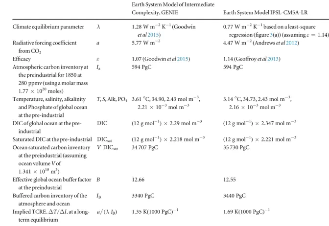
Table 1. Climate variables in the two Earth System Models of different complexity. Earth System Model of Intermediate

Complexity, GENIE Earth System Model IPSL-CM5A-LR Climate equilibrium parameter λ 1.28 W m−2K−1(Goodwin

et al2015)

0.77 W m−2K−1based on a least-square regression(figure3(a)) (assuming ε=1.14) Radiative forcing coefficient

from CO2

a 5.77 W m−2 4.47 W m−2(Andrews et al2012) Efficacy ε 1.07(Goodwin et al2015) 1.14(Geoffroy et al2013) Atmospheric carbon inventory at

the preindustrial for 1850 at 280 ppmv(using a molar mass 1.77×1020_moles)

Ia 594 PgC 594 PgC

Temperature, salinity, alkalinity and Phosphate of global ocean at the pre-industrial

T, S, Alk, PO4 3.61°C, 34.90, 2.43 mol m−3,

2.21×10−3mol m−3

3.14°C, 34.73, 2.43 mol m−3, 2.16×10−3mol m−3 DIC of global ocean at the

pre-industrial

DIC (12 g mol−1)×2.29 mol m−3 (12 g mol−1)×2.347 mol m−3

Saturated DIC at the pre-industrial DICsat (12 g mol−1)×2.218 mol m−3 (12 g mol−1)×2.221 mol m−3

Ocean saturated carbon inventory at the preindustrial(assuming ocean volume V of

1.341×1018m3)

V DICsat 34 707 PgC 35 730 PgC

Effective global ocean buffer factor at the preindustrial

B 12.66 12.55

Buffered carbon inventory of the atmosphere and ocean

IB 3340 PgC 3440 PgC

Implied TCRE,ΔT/ΔI, at a long-term equilibrium

3.1. Earth System Model configurations

The Earth System Model of Intermediate Complexity (GENIE) is configured as a coarse-resolution atmos-phere–ocean system, containing coupled circulation and biogeochemistry with 16 ocean layers and 36×36 equal-area grid elements over the globe (Ridgwell et al2007). This version of GENIE includes

climate feedbacks, in which increased CO2increases

the radiative forcing and warms the climate; in this application of GENIE, sediment interactions are disabled. The model configurations are forced to reproduce historical CO2concentrations to 2005 and

then to follow Representative Concentration Pathways (RCPs, Moss et al2010) until 2100 for those RCPs with

significant warming (RCP 4.5, 6.0 and 8.5).

IPSL-CM5A-LR is an ocean–atmosphere general circulation model including an explicit representation of the carbon cycle on land and in the ocean(Dufresne et al 2013). In this version, the atmospheric

comp-onent(LMDZ) is integrated with 39 vertical levels and a horizontal resolution of 3.75°×1.9°, and the ocea-nic component(NEMOv3.2) is integrated with 31 ver-tical levels and a horizontal resolution ranging from 0.5° to 2°. For the simulations diagnosed here, the model is forced with prescribed atmospheric CO2

concentrations, following historical CO2values until

2005, and the different RCP from 2005 to 2100; RCP 2.6, 4.5, 6.0 and 8.5. Other forcings, such as land-use changes, other greenhouse gases and anthropogenic aerosols are also included.

The carbon cycle components, ORCHIDEE for the land (Krinner et al 2005) and PISCES for the

ocean(Aumont and Bopp2006), provide net carbon

fluxes from the atmosphere to the terrestrial bio-sphere and the ocean, respectively. These fluxes include the net effect of changing atmospheric CO2

and those of climate feedbacks. Compatible anthro-pogenic emissions are diagnosed a posteriori, using modelled air-to-sea and air-to-land carbonfluxes as well as imposed atmospheric CO2 trajectories, as

applied in Jones et al(2013).

3.2. Assessment using an Earth System Model of Intermediate Complexity

The transient climate response is now assessed using GENIE, configured as an idealised atmosphere–ocean model; see Goodwin et al (2015) for further model

details. There is only radiative forcing from atmo-spheric CO2with no changes to other radiative forcing

agents, such as aerosols, and no changes in the terrestrial sink of carbon, so that the TCRE depend-ence in(12) simplifies to T I a I N t R t I t I t TCRE 1 1 . 15 B Usat ( ) ( ) ( ) ( ) ( ) ⎛ ⎝ ⎜ ⎞ ⎠ ⎟⎛ ⎝ ⎜ ⎞ ⎠ ⎟ l e = D D = - D + D

Within GENIE, the equilibrium TCRE from

a/(lIB) is given by 1.35 K(1000 PgC)−1, where

a=5.35 W m−2, λ=1.28 W m−2K−1 and IB=3340 PgC (table1). The efficacy factor weighting

the effect of the ocean heatflux on surface temperature is 1.07(table1; Goodwin et al2015).

The temporal evolution of the TCRE is deter-mined by(i) how the dependence of surface warming on radiative forcing,DT/DR,varies with the normal-ised ocean heat uptake, N te ( )/DR t ,( ) versus(ii) how the dependence of radiative forcing from atmospheric CO2on carbon emissions,DRCO2/DI,varies with the

normalised ocean undersaturation in car-bon, IUsat( )t /DI t( ).

Within the GENIE model, the dependence of sur-face warming on radiative forcing,DT/DR,increases in time(figure2(a)). This increase in TD /DRis due to changes in ocean heat uptake as the ocean interior warms and its temperature increases from its pre-industrial state; the ocean surface temperature then increases more rapidly for a specified increase in radia-tive forcing, since a smaller fraction of the radiaradia-tive forcing is taken up by the ocean heatflux to warm the ocean interior. This response is equivalent to surface warming leading to a thinning of the surface mixed layer and increasing the stratification in the underlying ocean interior.

The dependence of radiative forcing from atmo-spheric CO2 on carbon emissions, DRCO2/DI,

decreases in time (figure 2(b)). This decrease in RCO2 I

D /D is due to the ocean taking up carbon, so that the ocean carbon undersaturation decreases. The increase in radiative forcing from atmospheric CO2

then becomes smaller for additional increases in emit-ted carbon with a smaller change in the logarithm of CO2 induced per unit carbon emitted through the

decrease in ocean undersaturation.

In consequence, there is a relatively small decrease in the TCRE (figure 2(c)) through a slightly larger

decrease inDRCO2/DIbeing partly compensated by a

smaller increase inDT/DR.There is only a relatively weak sensitivity to emission pathway on this cen-tennial timescale (different coloured lines in figure1(a), left panel and figure2).

3.3. Assessment using an Earth System Model In the more complex Earth System Model IPSL-CM5A-LR, the warming response is explored for four RCP emissions scenarios(figure1(a), right panel). The

climate projections are affected also by non-CO2

radiative forcing, including changes from anthropo-genic aerosols, non-CO2greenhouse gases, land-use

changes and terrestrial changes in carbon storage. Accordingly, the TCRE is now diagnosed using the full expression in(11).

3.3.1. Equilibrium response

Our theory suggests that the TCRE asymptotes to an equilibrium response given by the time-independent factors a/(lI ,B) each of these input parameters differ

inventory IBis diagnosed as 3440 PgC, similar to the

estimate of 3340 PgC for GENIE(table1). The climate

parameter is diagnosed as l =0.77W m−2K−1 by solving a least-squares regression of the surface heat balance(Gregory et al2004); comparing the time series

of the radiative forcing minus ocean heat uptake,

R eN

D - (W m−2_{), versus surface temperature}

change,ΔT (K) (figure3(a), table2). Our estimate of

the climate parameter,λ, is very close to estimates of 0.75, 0.76 and 0.79 W m−2K−1 based on climate-model projections for an abrupt 4×CO2 increase,

respectively, from Andrews et al(2012), Dufresne et al

(2013) and Geoffroy et al (2013). The climate

para-meter,λ, is assumed to remain constant over time and is evaluated over the climate model integrations to 2100, rather than from an integration to an equili-brium state: the resulting values ofλ vary with the RCP scenario(table 2), which might possibly reflect

a time-dependence in its response (Senior and

Mitchell2000) or a sensitivity to regional changes in

warming and ocean circulation that differ with each RCP(Armour et al2013, Winton et al2013).

The coefficient for the radiative forcing depend-ence on atmospheric CO2, a, is taken as 4.47 W m−2

from the effective radiative forcing diagnosed for a climate model projection with an abrupt 4×CO2

increase(Andrews et al2012). This effective radiative

forcing estimate is less than the expected theoretical value of 5.35 W m−2 (Myhre et al 1998) and takes

into account rapid adjustments in clouds and other tropospheric and land-surface changes (Forster et al2013).

The diagnosed values of a,λ and IB, then suggest

an equilibrium dependence of surface warming to cumulative carbon emissions for the Earth System Model of 1.69 K(1000 PgC)−1, slightly larger than the equilibrium dependence of 1.35 K(1000 PgC)−1 _for

GENIE(table1).

Figure 2. Diagnostics of the GENIE Earth System Model for historical and 3 RCP scenarios(RCP 4.5, 6.0 and 8.5) from 2005 to 2100: (a) the dependence of surface warming on radiative forcing,DT/DR;(b) the dependence of radiative forcing from atmospheric CO2

on cumulative carbon emissions,DRCO2/DI;(c) the TCRE, the dependence of surface warming on cumulative carbon emissions, T I.

D /D In this model, the radiative forcing is only due to the contribution of atmospheric CO2. The right-hand axes display the

normalised values of each climate-dependence according to our expected equilibrium response, where the value of 1 refers to the long-term equilibrium value.

3.3.2. Transient response

To understand the transient response, the different terms in the global heat balance (6) and buffered

carbon inventory(8) are diagnosed. The heat flux into

the climate system, N(t), is equated with the ocean heat heat uptake, and diagnosed from the tendency in the global ocean heat content. The ocean carbon

undersaturation, IUsat(t), is diagnosed from the

differ-ence in the saturated DIC anomaly and the actual DIC anomaly over the global ocean, IUsat( ) =t V(DDICsat( )t - DDIC( ))t .

There are temporal variations in the surface heat balance(6) over the 100 year integration. The radiative

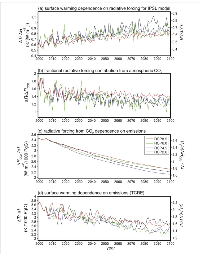
forcing,ΔR(t), is dominated by the contribution from Figure 3. Diagnostics of IPSL-CM5A-LR simulations for the surface heat balance and buffered carbon inventory from 2005 to 2100: (a) scatterplot showing the relationship between the radiative forcing minus ocean heat uptake,D -R eN(W m−2) versus surface

temperature change,_{ΔT (K), for RCP2.6, RCP4.5, RCP6.0 and RCP8.5. A least squares fit to the slope provides an estimate of the} climate parameterλ with a mean value of 0.77 W m−2K−1for the four RCPs(table2); this scatterplot is for an efficacy ε of 1.14 (Geoffrey et al2013); (b) temporal variation of the surface heat balance (W m−2) for RCP8.5 (assuming λ=0.77 W m−2K−1and ε=1.14). The radiative forcing ΔR(t) (black line) is mainly from the effect of atmospheric CO2(black dashed line). The radaitive

forcingΔR(t) is partly offset by an ocean heat uptake N(t) (blue line), and the resulting net heating drives the climate response of a surface warming and increase in outgoing longwave radiation,λΔT(t) (red line). At the start of the integration, the climate response is slightly less than the ocean heat uptake, while by the end of the integration, the climate response slightly exceeds the ocean heat uptake. Thus, the dependence of surface warming on radiative forcing increases in time. In(c), accompanying temporal changes in the carbon inventory(PgC) for carbon emission (red line), ocean undersaturation (blue line) and change in terrestrial store (green line) together with the change in the log of atmospheric CO2(black dashed line) that balances the sum of the inventory changes normalised by

IB=3440 PgC (right axis). The climate emission is initially comparable to the ocean undersaturation, but then proceeds to exceed the

ocean undersaturation as the ocean sequesters carbon from the atmosphere. Thus, the dependence of radiative forcing from atmospheric CO2on carbon emissions decreases in time.

atmospheric CO2, DRCO2( )t (figure 3(b), black full

and dashed lines for RCP8.5). The radiative forcing, ΔR(t), is partly offset by an ocean heat uptake, N(t) (blue line), and the remaining net forcing drives the surface climate response, λΔT(t) (red line) in figure 3(b); assuming ε=1.14 from Geoffroy et al

(2013). At the start of the integration, the climate

response is slightly less than the ocean heat uptake, while by the end of the integration, the climate response is slightly larger than the ocean heat uptake. Thus, the normalised ocean heat uptake,

N t( ) R t ,( )

e /D decreases in time in(11), leading to the

dependence of surface warming on radiative forcing increasing in time.

There are likewise temporal changes in the buf-fered carbon balance(8), although the carbon

inven-tory changes are noticeably smoother. The ocean carbon undersaturation, IUsat(t) (blue line), is initially

comparable to the cumulative carbon emission,ΔI(t) (red line), but becomes slightly smaller over the 100 year integration infigure 3(c). Thus, the normalised

ocean undersaturation, IUsat(t)/ΔI(t), reduces in time

and there is also a relatively small increase in the ter-restrial store of carbon, ΔIter (t) (figure 3(c), green

line). Thus, I(Usat( )t - DIter( ))t /DI t( ) reduces in

time in(11), leading to the dependence of radiative

forcing on carbon emissions decreasing in time. Accordingly, there are larger centennial trends for the dependencies making up the TCREall R, than for

the TCREall R: there is a long-term increase in the

dependence of surface warming on radiative forcing,

T R

D /D (figure4(a)), a smaller decrease in the

frac-tional dependence of radiative forcing from atmo-spheric CO2, DR/DRCO2(figure 4(b)), and a larger

decrease in the dependence of radiative forcing on car-bon emissions,DRCO2/DI(figure4(c)). The resulting

TCREall Rthen only slightly decreases over the

cen-tennial timescale(figure4(d)).

There are though decadal changes in the TCREall R

(figure4(d)). The decadal variability in TD /DI origi-nates from decadal changes in the dependence of surface warming on radiative forcing, DT/DR

(figure 4(a)) from changes in ocean heat uptake

(figure3(b), blue line), and the fractional dependence

of radiative forcing on atmospheric CO2,DR/DRCO2

(figure4(b)) from the effects of aerosols and non-CO2

greenhouse gases. In contrast, the dependence of radiative forcing from atmospheric CO2 on carbon

emissions, DRCO2/DI, varies relatively smoothly

in time(figure 4(c)) due to the smooth changes in

carbon emissions and ocean carbon undersaturation (figure3(c), red and blue lines).

3.4. Comparison of Earth System Models of different complexity

Our framework for the TCREall Rhighlights how there

are broadly similar responses in the Earth System Models, GENIE and IPSL-CM5A-LR. The centennial trends of the TCREall R and its dependences have

similar signs to each other in both Earth System Models(figures2and4): both models show a positive

trend in the dependence of surface warming on radiative forcing, a negative trend in the dependence of radiative forcing on carbon emissions, and a resulting slight negative trend in the TCRE. Thus, there is traceability between these Earth System Models of different complexity, as there are similar underlying trends in their response.

The exact values of the dependences differ though in each Earth System Model(table3), as the models

contain different representations of the physical circu-lation and biogeochemistry. The TCREall Ris higher in

the IPSL-CM5A-LR model, than in GENIE, and sub-sequently reduces by a greater amount over the next century(table3). These differences in the TCREall Rare

due to(i) a larger dependence of the surface warming on radiative forcing in IPSL-CM5A-LR than in GENIE, and(ii) conversely a smaller dependence of the radiative forcing from atmospheric CO2on

cumu-lative emissions in IPSL-CM5A-LR than in GENIE. There are also interannual and decadal differences in each model due to the IPSL-CM5A-LR containing radiative forcing contributions from aerosols and non-CO2greenhouse gases, as well as more complex

ocean dynamics altering the ocean uptake of heat and carbon.

There are only slight differences in each of the climate dependences for the different choices of the RCP emission pathways over a century timescale (figures1(a),2and4; table3).

4. Discussion

Our framework to understand the variation of the TCRE draws upon the fundamental link between the logarithm of atmospheric CO2and the definitions of

the radiative forcing from atmospheric CO2(5) and a

buffered carbon inventory(6) accounting for ocean

carbonate chemistry. Table 2. Estimates of the climate parameterλ from the Earth System

Model IPSL-CM5a-LR for emission pathways: RCP2.6, RCP4.5, RCP6.0 and RCP8.5. The climate parameter is estimated from a least squaresfit between the radiative forcing minus ocean heat uptake,

R eN

D - (W m−2_{) and surface temperature change ΔT (K) for an}

efficacy ε of 1.14 (Geoffrey et al2013). The average value of λ for all RCPs is 0.77; all correlation coefficients are significant (r>0.26 for a 99% confidence limit).

Climate parameter Correlation coef_ficient Emission pathway λ (W m−2K−1) r

RCP 2.6 1.02 0.78

RCP 4.5 0.76 0.92

RCP 6 0.68 0.86

4.1. Alternative frameworks

There are two alternative approaches to our frame-work. Firstly, the TCRE has been previously explained in terms of the dependence of surface temperature on atmospheric CO2, DT/DCO ,2 multiplied by the

dependence of atmospheric CO2on cumulative

emis-sions, DCO2/DI (Matthews et al 2009, Gillett

et al2013). Their approach highlights how the TCRE is

nearly constant due to partial compensation between

changes in the dependence of surface temperature on CO2and changes in the air-borne fraction of emitted

carbon.

Secondly, the sensitivities of climate models have been understood in terms of empirical parameters,α, β and γ, representing the sensitivity of temperature to atmospheric CO2, and the sensitivity of carbon

inve-tories to atmospheric CO2 and temperature

respec-tively(Friedlingstein et al2006, Plattiner et al2008).

Figure 4. Diagnostics of IPSL-CM5A-LR simulations for historical and 4 RCP scenarios(RCP 2.6, 4.5, 6 and 8.5) from 2005 to 2100: (a) dependence of surface warming on effective radiative forcing,DT/DR(K W−1m−3); (b) fractional radiative forcing contribution from atmospheric CO2,DR/DRCO2;(c) dependence of radiative forcing from CO2on carbon emissions,DRCO2/DI(W m−2/

1000 PgC) and (d) the TCREall R, the dependence of surface warming on carbon emissions,DT/DI(K/1000 PgC) versus time. The

right-hand axes display the normalised values of each climate-dependence according to our expected equilibrium response, where the value of 1 refers to the long-term equilibrium value. Note that the vertical range in(a) and (d) are a factor 2 larger than in figure2.

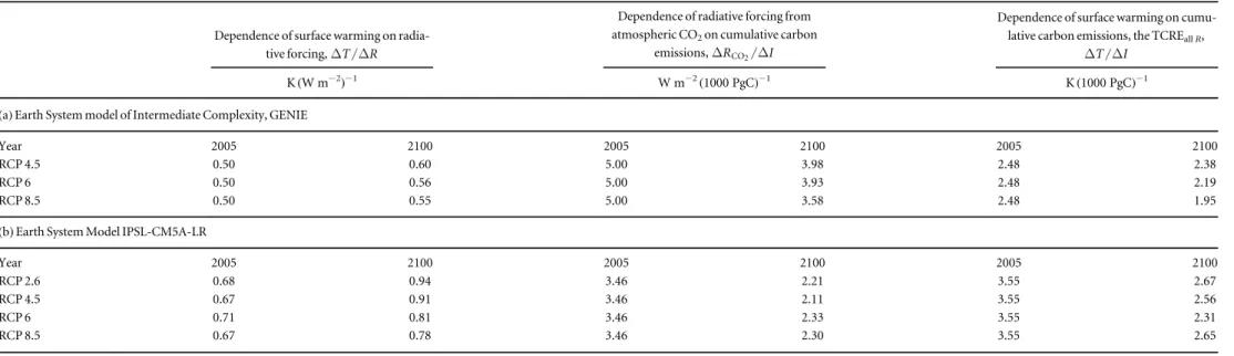
Table 3. Climate dependences for two Earth System Models at 2005 and 2100 for different choices of emission pathways.

Dependence of surface warming on radia-tive forcing,DT/DR

Dependence of radiative forcing from atmospheric CO2on cumulative carbon

emissions,DRCO2/DI

Dependence of surface warming on cumu-lative carbon emissions, the TCREall R,

T I

D /D

K_{(W m}−2₎−1 W m−2_{(1000 PgC)}−1 K_{(1000 PgC)}−1

(a) Earth System model of Intermediate Complexity, GENIE

Year 2005 2100 2005 2100 2005 2100

RCP 4.5 0.50 0.60 5.00 3.98 2.48 2.38

RCP 6 0.50 0.56 5.00 3.93 2.48 2.19

RCP 8.5 0.50 0.55 5.00 3.58 2.48 1.95

(b) Earth System Model IPSL-CM5A-LR

Year 2005 2100 2005 2100 2005 2100 RCP 2.6 0.68 0.94 3.46 2.21 3.55 2.67 RCP 4.5 0.67 0.91 3.46 2.11 3.55 2.56 RCP 6 0.71 0.81 3.46 2.33 3.55 2.31 RCP 8.5 0.67 0.78 3.46 2.30 3.55 2.65 11 Res. Lett. 11 (2016 ) 015003

This approach has been used to understand the con-tributions of the different land and ocean inventories to carbon uptake and feedback on climate.

In our view, the connection to the underlying the-ory is more transparent in our framework, since there are clear dependences on the logarithm of atmo-spheric CO2drawing upon the buffered carbon

inven-tory(8) and the definition of radiative forcing from

atmospheric CO2 in (9). While our framework

includes a term accounting for changes in the terres-trial carbon sink, our theory is designed to make clearer the central contribution of the ocean, rather than drawing upon empirical relationships between changes in the land sinks of carbon (Friedlingstein et al2006).

4.2. Mechanistic control of the TCRE

The long-term trends for the TCRE can be simply understood in terms of the heat and carbon uptake for an idealised representation of the atmosphere–ocean-terrestrial system. The additional heat supplied to the climate system is primarily taken up by the ocean, while the additional carbon is taken up by both the ocean and terrestrial system.

In order to understand how the TCRE is con-trolled, now consider how the climate response to car-bon emissions is likely to alter in time:

(i) the additional heat supplied from an increase in radiative forcing is used to warm both the surface and ocean interior. As the ocean interior warms in time, a smaller proportion of the radiative forcing is taken by

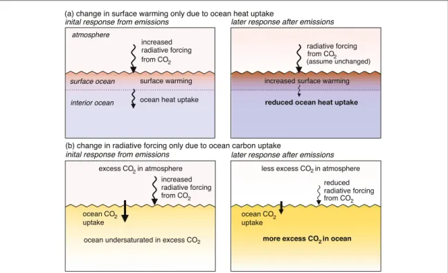
the interior and a larger proportion of the radiative forcing then warms the surface. Thus, the dependence of surface warming on radiative forcing,DT/DR,is expected to increase in time as the ocean interior adjusts to a new equilibrium (figure 5(a)).

Equiva-lently, the radiative forcing is likely to increase the stra-tification in time and lead to an increase in the dependence of surface warming on radiative forcing.

(ii) For a given carbon emission, radiative forcing is initially expected to be large as most of the emitted carbon is in the form of atmospheric CO2. The

radia-tive forcing is then expected to decline as the excess atmospheric CO2is taken up by the ocean and

terres-trial system. Thus, the dependence of radiative forcing from atmospheric CO2 on cumulative carbon

emis-sions,DRCO2/DI,is expected to decrease in time as

the ocean and terrestrial system take up the excess atmospheric CO2(figure5(b)).

(iii) The resulting surface warming response to cumulative carbon emissions (the TCRE) then only weakly varies, depending on the partial compensation between the dependences of surface warming on radiative forcing,DT/DR,and the radiative forcing from atmospheric CO2on emissions,DRCO2/DI.

This inference supports the argument of Solomon et al(2009) as to why long-term irreversible climate

change persists after the cessation of carbon emissions; the gradual reduction in radiative forcing from atmo-spheric CO2 is partly compensated by a decline in

ocean heat uptake, so that global warming is likely to continue to persist on a millennial timescale.

Figure 5. Schematic view of how the ocean affects the surface warming response to carbon emissions in time:(a) the dependence of surface warming on radiative forcing,DT/DR,increases as ocean heat uptake declines;(b) the dependence of radiative forcing from atmospheric CO2on carbon emissions,DRCO2/DI,declines as the ocean takes up more excess CO2in the atmosphere. The resulting

changes in the TCRE are due to a partial compensation between(a)DT/DRincreasing in time and(b)DRCO2/DIdecreasing in time

4.3. Decadal variability

The decadal changes in the TCREallRcan be

under-stood via our relationship (11). The dependence of

surface warming on radiative forcing, DT/DR, is controlled by the heatflux from the atmosphere to the ocean weighted by the efficacy, such that

1 . T R N t R t 1

(

)

¶ D The magnitude and sign of the

ocean heat flux (figure 3(b), blue line) can easily

change on interannual to decadal timescales given changes in atmosphere and ocean heat storage. For example, there is a hiatus in surface warming for 2000–2010, which is attributed to an increase in ocean heat uptake(Guemas et al2013, Watanabe et al2013).

These changes in ocean heat uptake might be asso-ciated with coupled atmosphere–ocean phenomena, such as the El Nino Southern Oscillation, or changes in ocean ventilation, particularly associated with formation of water masses in the North Atlantic and Southern Ocean.

The dependence of radiative forcing on the contribution from atmospheric CO2, DR/DRCO2

(figure 4(c)) can likewise easily alter through the

release of atmospheric aerosols, particularly linked to volcanic and anthropogenic emissions (Ottera et al 2010, Booth et al 2012), and changes in other

non-CO2 greenhouse gases, such as methane

(Pierrehumbert2014).

The dependence of radiative forcing from CO2on

carbon emissions, DRCO2/DI, is controlled by the

carbon undersaturation of the ocean relative to the atmosphere and changes in the terrestrial sink of

car-bon, R 1 . I a I I t I t I t I t CO2 B Usat ter

(

)

undersaturation of the ocean, IUsat(t), only alters

slowly in time(figure3(c), blue line) and is less

sensi-tive to the interannual and decadal changes in the car-bonflux between the atmosphere and ocean, such as seen in climate model simulations of natural varia-bility in air-sea CO2 and O2 fluxes (Resplandy

et al2015). The terrestrial sink probably weakly

increa-ses in time,ΔIter(t) (figure3(c), green line), although

there is a large range in the magnitude and sign in the projected terrestrial response for different climate models(Friedlingstein et al2006).

5. Conclusions

The mechanisms controlling the TCRE from all radiative forcings are revealed here in a new frame-work, formulated in terms of the product of three climate dependences in(5): the dependence of surface

warming on radiative forcing,DT/DR,the fractional dependence of radiative forcing from atmospheric CO2, DR/DRCO2, and the dependence of radiative

forcing from atmospheric CO2on carbon emissions,

RCO2 I D /D : T I T R R R R I TCREallR . CO CO 2 2 ⎜ ⎟ ⎛ ⎝ ⎞ ⎠ ⎛ ⎝ ⎜ ⎞ ⎠ ⎟⎛_⎝⎜ ⎞_⎠⎟ = D D = D D D D D D This definition of the TCREallRcan then be

expres-sed in terms of an equilibrium response multiplied by three time-dependent terms in(11): depending on the

damping of surface warming due to ocean heatflux, the enhancement of atmospheric CO2due to carbon

undersaturation of the ocean and terrestrial system, and the fractional dependence of radiative forcing on atmospheric CO2: a I N t R t I t I t I t I t R t R t TCRE 1 1 . R all B Usat ter CO2 ( ) ( ) ( ) ( ) ( ) ( ) ( ) ( ) ⎛ ⎝ ⎜ ⎞_⎠⎟ ⎛ ⎝ ⎜ ⎞_⎠⎟⎛ ⎝ ⎜ ⎞ ⎠ ⎟ l e = -D ´ + D -D D D D

Applying this framework, the near constancy of the TCRE on multi-decadal to centenial timescales is explained by a partial compensation between the effects of ocean heat and carbon uptake on the depen-dences of surface warming on radiative forcing and radiative forcing from atmospheric CO2 on carbon

emissions. The dependence of surface warming on emissions then remains nearly constant, since the dependence of surface warming on radiative forcing is enhanced as ocean heat uptake declines, but at the same time the dependence of radiative forcing on car-bon emissions is reduced as the ocean takes up excess CO2 in the atmosphere(Goodwin et al2015). Thus,

this climate response primarilly depends on the physi-cal mechanisms by which the ocean sequesters heat and carbon, involving the physical transport of surface waters into the ocean interior.

There is no need though for the ocean sequestering of heat and carbon to always mirror each other and the TCRE can respond differently to rapid or slow rates of emissions given sufficient time (Krasting et al2014), as

well as be affected by changes in ocean circulation (Winton et al2013) and regional feedbacks (Armour

et al2013). There may even be continued global

warm-ing after carbon emissions cease(Frölicher et al2014)

due to the warming effect of decreasing ocean heat uptake exceeding the cooling effect of decreasing atmospheric CO2.

The TCRE from all radiative forcing can easily vary on decadal timescales through changes in the sign of the annual ocean heat uptake and changes in radiative forcing from non-CO2contributions, such as aerosols

and other greenhouse gases.

In summary, our framework for the TCRE and link to underlying theory provides an alternative way to interpret the response of climate models and under-stand how the climate models are mechanistically con-trolled. The ocean is providing a central role in controlling the TCRE through the uptake of heat and carbon in the climate system. The framework can also be used to provide traceability between simple and complex models, and understand the underlying

cause for their different responses. The robustness of the TCRE on centennial timescales also supports the view that cumulative carbon emissions provides a pol-icy framework for reducing adverse climate change (Matthews et al2012).

Acknowledgments

This work was supported by a UK Natural Environ-ment Research Council grant, NE/K012789/1. We thank two anonymous referees for constructive com-ments that strengthened the work.

References

Allen M R et al 2009 Warming caused by cumulative carbon emissions towards the trillionth tonne Nature458 1163–6 Andrews T, Gregory J M, Webb M J and Taylor K E 2012 Forcing,

feedbacks and climate sensitivity in CMIP5 coupled atmosphere_{–ocean climate models Geophys. Res. Lett.}39 L09712

Armour K C, Bitz C M and Roe G H 2013 Time-varying climate sensitivity from regional feedbacks J. Clim.26 4518–34 Aumont O and Bopp L 2006 Globalizing results from ocean insitu

iron fertilization studies Glob. Biogeochem. Cycles20 GB2017 Booth B B B et al 2012 Aerosols implicated as a prime driver of

twentieth-century North Atlantic climate variability Nature 484 228–32

Church J A et al 2011 Revisiting the Earth’s sea-level and energy budgets from 1961 to 2008 Geophys. Res. Lett.38 L18, 601, 794 Collins M et al 2013 Long-term climate change: projections,

commitments and irreversibility Climate Change 2013: The Physical Science Basis, Contribution of Working Group I to the Fifth Assessment Report of the Intergovernmental Panel on Climate Change ed T F Stocker et al(Cambridge: Cambridge University Press₎

Dufresne J L et al 2013 Climate change projections using the IPSL-CM5 Earth System Model: from CMIP3 to CMIP5 Clim. Dyn. 40 2123–65

Follows M J, Dutkiewics S and Ito T 2006 On the solution of the carbonate system in ocean biogeochemical models Ocean Model12 290–301

Forster P M et al 2013 Evaluating adjusted forcing and model spread for historical and future scenarios in the CMIP5 generation of climate models J. Geophys. Res.118 1139–50

Friedlingstein P et al 2006 Climate-carbon cycle feedback analysis: result from the C4MIP model intercomparison J. Clim.19 3337–53

Frölicher T L, Winton M and Sarmiento J L 2014 Continued global warming after CO2emissions stoppage Nat. Clim. Change4

40–4

Geoffroy O, Saint-Martin D, Bellon G and Voldoire A 2013 Transient climate response in a two-layer energy-balance model:II. Representation of the ef_{ficacyofdeep-oceanheatuptakeand} validation for CMIP5 AOGCMs J. Clim.26 1859_–76 Gillet N P, Arora V K, Matthews D and Allen M R 2013 Constraining

the ratio of global warming to cumulative CO2emissions

using CMIP5 simulations J. Clim.26 6844–58 Goodwin P, Williams R G, Follows M J and Dutkiewicz S 2007

Ocean–atmosphere partitioning of anthropogenic carbon dioxide on centennial timescales Glob. Biogeochem. Cycles21 GB1014

Goodwin P, Williams R G and Ridgwell A 2015 Sensitivity of climate to cumulative carbon emissions due to compensation of ocean heat and carbon uptake Nat. Geosci.8 29–34 Gregory J M, Ingram W J, Palmer M A, Jones G S, Stott P A,

Thorpe R B, Lowe J A, Johns T C and Williams K D 2004 A new method for diagnosing radiative forcing and climate sensitivity Geophys. Res. Lett.31 L03205

Gregory J M and Forster P M 2008 Transient climate response estimated from radiative forcing and observed temperature change J. Geophys. Res.113 D23105

Guemas V, Doblas-Reyes F J, Andreu-Burillo I and Asif M 2013 Retrospective prediction of the global warming slowdown in the past decade Nat. Clim. Change3 649–53

Hansen J, Lacis A, Rind D, Russell G, Stone P, Fung I, Ruedy R and Lerner J 1984 Climate sensitivity: analysis of feedback mechanisms Climate Processes and Climate Sensitivity(AGU Geophysical Monograph 29, Maurice Ewing) vol 5 ed J E Hansen and T Takahashi(Washington, DC: American Geophysical Union) pp 130–63

Jones C et al 2013 Twenty-first-century compatible CO2emissions

and airborne fraction simulated by CMIP5 Earth System Models under four representative concentration pathways J. Clim.26 4398–413

Knutti R and Hegerl G C 2008 The equilibrium sensitivity of the Earth’s temperature to radiation changes Nat. Geosci.1 735_–43

Krasting J P, Dunne J P, Shevliakova E and Stouffer R J 2014 Trajectory sensitivity of the transient climate response to cumulative carbon emissions Geophys. Res. Lett.41 2520–7 Krinner G et al 2005 A dynamic global vegetation model for studies

of the coupled atmosphere–biosphere system Glob. Biogeochem. Cycles19 GB1015

Matthews H R, Gillett N P, Stott P A and Zickfeld K 2009 The proportionality of global warming to cumulative carbon emissions Nature459 829–33

Matthews H R, Solomon S and Pierrehumbert R 2012 Cumulative carbon as a policy framework for achieving climate stabilization Phil. Trans. R. Soc. A370 4365–79 Moss R H et al 2010 The next generation of scenarios for climate

change research and assessment Nature463 747–56 Myhre G, Highwood E J, Shine K P and Stordal F 1998 New

estimates of radiative forcing due to well mixed greenhouse gases Geophys. Res. Lett.25 2715_–8

Ottera O H et al 2010 External forcing as a metronome for Atlantic multidecadal variability Nat. Geosci.3 688_–94

Pierrehumbert R T 2014 Short-lived climate pollution Annu. Rev. Earth Planet. Sci.42 341–79

Plattiner G-K et al 2008 Long-term climate commitments projected with climate-carbon cycle models J. Clim.21 2721–51 Resplandy L, Séférian R and Bopp L 2015 Natural variability

of CO2and O2fluxes: What can we learn from centuries-long

climate models simulations? J. Geophys. Res. Oceans120 384–404

Ridgwell A et al 2007 Marine geochemical data assimilation in an efficient earth system model of global biogeochemical cycling Biogeosciences4 87–104

Senior C A and Mitchell J F B 2000 The time-dependence of climate sensitivity Geophys. Res. Lett.27 2685–8

Solomon S, Plattner G-K, Knutti R and Friedlingstein P 2009 Irreversible climate change due to carbon dioxide emissions Proc. Natl Acad. Sci. USA106 1704_–9

Watanabe M, Kamae Y, Yoshimori M, Oka A, Sato M, Ishii M, Mochizuki T and Kimoto M 2013 Strengthening of ocean heat uptake efficiency associated with the recent climate hiatus Geophys. Res. Lett.40 3175–9

Williams R G and Follows M J 2011 Ocean Dynamics and the Carbon Cycle: Principles and Mechanisms(Cambridge: Cambridge University Press) p 416

Williams R G, Goodwin P, Ridgwell A and Woodworth P L 2012 How warming and steric sea level rise relate to cumulative carbon emissions Geophys. Res. Lett.39 L19715

Winton M, Takahashi K and Held I M 2010 Importance of ocean heat uptake efficacy to transient climate change J. Clim.23 2333–44

Winton M, Griffies S M, Samuels B L, Sarmiento J L and Frölicher T L 2013 Connecting changing ocean circulation with changing climate J. Clim.26 2268–78

Zickfeld K, Eby M, Matthews H D and Weaver A J 2009 Setting cumulative emissions targets to reduce the risk of dangerous climate change Proc. Natl Acad. Sci. USA106 16129_–34