Constructive global analysis of hybrid systems

(1)

Constructive Global Analysis of Hybrid Systems

by

Jorge Manuel Mendes Silva

Gongalves

Submitted to the Department of Electrical Engineering and Computer

Science

in partial fulfillment of the requirements for the degree of

Doctor of Philosophy

at the

MASSACHUSETTS INSTITUTE OF TECHNOLOGY

September 2000

©

Massachusetts Institute of Technology 2000. All rights reserved.

Author .

Depalment of Electrical Engineering and Computer Science

August 29, 2000

Certified by..

Al4

(7 .

Certified by...

.

_..../

Munther A. Dahleh

Professor

Thesis Supervisor

...

Alexandre Megretski

Associate Professor

- ---

In !-

i S

ervisor

Accepted by... ... ...

Arthur C. Smith

Chairman, Department Committee on Graduate Students

MASSACHUSETTS INSTITUTE OF TECHNOLOGY

OCT 2 3 2000

.... UBRARIES

BARKER

(2)

(3)

Constructive Global Analysis of Hybrid Systems

by

Jorge Manuel Mendes Silva Gongalves

Submitted to the Department of Electrical Engineering and Computer Science on August 29, 2000, in partial fulfillment of the

requirements for the degree of Doctor of Philosophy

Abstract

Many systems of interest are dynamic systems whose behavior is determined by the interaction of continuous and discrete dynamics. These systems typically contain variables or signals that take values from a continuous set and also variables that take values from a discrete, typically finite set. These continuous or discrete-valued variables or signals depend on independent variables such as time, which may also be continuous or discrete. Such systems are known as Hybrid Systems. Although widely used, not much is known about analysis of hybrid systems. This thesis attempts to take a step forward in understanding and developing tools to systematically analyze certain classes of hybrid systems. In particular, it focuses on a class of hybrid systems known as Piecewise Linear Systems (PLS). These are characterized by a finite number of affine linear dynamical models together with a set of rules for switching among these models. Even for simple classes of PLS, very little theoretical results are known. More precisely, one typically cannot assess a priori the guaranteed stability, robustness, and performance properties of PLS designs. Rather, any such properties are inferred from extensive computer simulations. In other words, complete and systematic analysis and design methodologies have yet - emerge.

In this thesis, we develop an entirely new constructive global analysis methodology for PLS. This methodology consists in inferring global properties of PLS solely by studying their behavior at switching surfaces associated with PLS. The main idea is to analyze impact maps, i.e., maps from one switching surface to the next switching surface. These maps are proven globally stable by constructing quadratic Lyapunov functions on switching surfaces. Impact maps are known to be "unfriendly" maps in the sense that they are highly nonlinear, multivalued, and not continuous. We found, however, that an impact map induced by an LTI flow between two switching surfaces can be represented as a linear transformation analytically parametrized by a scalar function of the state. Moreover, level sets of this function are convex subsets of linear manifolds. This representation of impact maps allows the search for quadratic Lyapunov functions on switching surfaces to be done by simply solving a set of LMIs. Global asymptotic stability of limit cycles and equilibrium points of PLS can this way be efficiently checked. The classes of PLS analyzed in this thesis are LTI systems in feedback with an hysteresis, an on/off controller, or a saturation. Although this analysis methodology yields only sufficient criteria of stability, it has shown to be very successful in globally analyzing a large number of examples with a locally stable limit

(4)

cycle or equilibrium point. In fact, existence of an example with a globally stable limit cycle or equilibrium point that could not be successfully analyzed with this new methodology is still an open problem. Examples analyzed include systems of relative degree larger than one and of high dimension, for which no other analysis methodology could be applied. We have shown that this methodology can be efficiently applied to not only globally analyze stability of limit cycles and equilibrium points, but also robustness, and performance of PLS. Using the same ideas, performance of on/off systems in the sense that bounded inputs generate bounded outputs, can also be checked. _{Among those on/off and saturation systems analyzed are systems with} unstable nonlinearity sectors for which classical methods like Popov criterion, Zames-Falb criterion, IQCs, fail to analyze. This success in globally analyzing stability, robustness, and performance of certain classes of PLS has shown the power of this new methodology, and suggests its potential towards the analysis of larger and more complex PLS.

Thesis Supervisor: Munther A. Dahleh Title: Professor

Thesis Supervisor: Alexandre Megretski Title: Associate Professor

(5)

To my Parents Dedicado aos meus Pais

(6)

(7)

Acknowledgments

Wow!... Is my thesis really finished? I cannot believe this is over. Somehow, it seems not that long ago since the day I first arrived to MIT. I guess when you enjoy what you do, time really flies. Looking back at the last few years, I cannot even start to put in words how my stay at MIT has changed my life. What I can say for sure is that I am not the same person that came here. I have improved in every aspect of my life, from professional to personal. Obviously, such changes do not happen by yourself. People around you influence you and change you in ways that you typically do not realize until many years later. Over the last years at MIT, I had the pleasure of meeting and interacting with many great people. I am just grateful that, consciously or not, I have learned so much from all of them, sometimes even the hard way.

I would like to thank my advisors Munther Dahleh and Alexandre Megretski. What else can I say about them? Just that they are the best advisors in the world, and I was lucky enough to find them. I would like to thank the members of my Thesis Committee Sanjoy Mitter and Eric Feron, and also George Verghese, Michael Athans, and John Tsitsiklis for their support.

Obviously, not only professors influenced my learning experience at MIT. I have been fortunate to benefit from helpful discussions with many graduate students and post-doctoral fellows at the Laboratory for Information and Decision Systems (LIDS). The numerous discussions about nearly anything with my officemates Sean Warnick, Fadi Karameh, and Marcos Escobar helped me keep my mind and soul in balance. I would also like to thank other colleagues in LIDS which I had the luck to have around to discuss and exchange research ideas: Nicola Elia, Isaac Kao, Georgios Kotsalis, Ulf J6nsson, Nuno Martins, Reza Olfati-Saber, and Fernando Paganini. Other students in LIDS that I would like to acknowledge: Ola Ayaso, Soosan Beheshti, Constantinos Boussios, Michael Branicky, Julio Castrillon, Kuang Han Chen, Emilio Frazzoli, John Harper, Venkatesh Saligrama, Sri Sarma. Still in LIDS, I want to thank the great support and help I had from Fifa Monserrate, Doris Inslee, Kathleen Sullivan, Monica Bell, and Marilyn Pierce.

As I mentioned, my stay at MIT changed me in many ways. Academically is just one of these ways. Outside the lab, many people have influenced me for the best. I want to thank Jacinto and Maria Figueiredo for making feel like I was at home. I especially thank everyone on my floor, Conner 3, for all these great years as a GRT on the best floor on campus. You guys are the best. In my dorm, I also want to thank Halston and Kathy Taylor, and Rosa and Manuel.

While a competitor ballroom dancer, I had the pleasure of making many friends that helped me keep my mind off MIT, even if just for a little while. Among them are Yumiko Osawa, David Johnson, Zoe Antoniou, Aamir Rashi, Wendy Luo, and, of course, Stephanie Kong.

I would like to thank Nuno Vasconcelos and Manuela Pereira for their constant support. Other friends that I was lucky to meet here are Jos6 Monteiro, Luis Silveira, Nuno Martins, Luisa Marcelino, Miguel and In~s Castro, Miguel and Helga Arsenio. Back home, I want to thank Jorge Reis Lima. If it was not for him, I would have never been here. I am happy that his incentives to apply and come to MIT were

(8)

strong enough. I also want to thank Fernando Lobo Pereira for his constant support and unconditional help.

My friends back home Vitor Seabra, Jos6 Paulo Sa, Luis Costa, Valter Henriques, Sergio Alexandre, Jodo Carlos, Eixo and many other members of the Tuna, Jodo Carlos Pimenta, Sergio Reis Cunha, Pedro Correia, Manuel Correia, Mario Valente, Silvia Lopes, and In~s Oliveira helped me greatly in making me believe I did the right thing in coming here in the first place, and have always made me feel at home when I go back on vacations.

Of all the people I have met while at MIT, there was one special person that had the most influence in making me a better person. Paula Waicman has showed me the world through different eyes, and for that I am truly thankful. We have shared incredible moments of happiness and joy that made my journey through MIT unforgettable. Undoubtfully, part of what I am today I owe it to her.

Of course, my family members have always given me tremendous and uncondi-tional support. I could have not done it without their support. In particular, I want to thank my sister Cristina, Mario Rui, and my adorable little nephews Rui Pedro and Rita Filipa, whom I miss greatly. And to the best parents in the world, from the bottom of my heart: Thank You. This thesis is dedicated to both of you.

Last, but not least, I want to acknowledge and thank the support of my research. This research was supported in part by the Portuguese "Fundagdo para a Ci~ncia e Tecnologia" under the program "PRAXIS XXI", by the NSF under grants ECS-9410531, ECS-9796099, ECS-9796033, and ECS-9612558 and by the AFOSR under grants F49620-96-1-0123, F49620-00-1-0096, AFOSR F49620-95-0219 and F49620-99-1-0320.

Jorge M. M. S. Gongalves August 29, 2000

(9)

List of Figures

1-1 1-2 1-3 1-4 1-5 1-6 1-7 1-8 1-9 1-10 1-11 1-12 1-13

Sampled data system . . . . Switching between different models . . . . Coulomb friction . . . . H ysteresis . . . . Saturation . . . . Mass-spring with damage protection . . . . Switching between different pairs of models/controllers Switching between different controllers . . . . Typical tire adhesion curve for brake control . . . . Different stages of a hopping monopod . . . . Closed trajectory switching among different systems . . 3rd-order system with unstable nonlinearity sector . . . On/Off System . . . . . . . . 20 . . . . 21 . . . . 22 . . . . 22 . . . . 23 . . . . 23 . . . . 24 . . . . 24 . . . . 24 . . . . 25 . . . . 26 . . . . 29 . . . . 29 3-1 Piecewise Linear System with a memoryless switching rule . . . . 3-2 Left-Saturation system; Right-state space cells . . . . 3-3 Relay Feedback System . . . . 3-4 Existence of solutions; from left to right: one, multiple, and no solutions 3-5 Lim it cycle -y . . . . 3-6 Periodic solution of a second-order PLS . . . . 3-7 PLS with limit cycles and equilibrium points . . . . 4-1 PLS composed of an unstable and a stable linear systems . . . . 4-2 Maps from one switching surface to the next switching surface . . . .

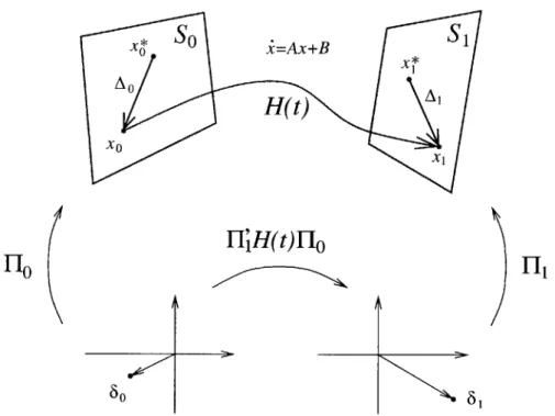
4-3 Impact map from Ao E Sod - X to A, E S' - x*...

4-4 Existence of multiple solutions . . . . 4-5 Map from Ao to A, is not continuous . . . . 4-6 Every point in St has a switching time of t . . . . 4-7 n - 1 dimensional map . . . . 4-8 So C So and S' C S1 are some sets defined to the right of t0 and 22,

respectively . . . . 4-9 Sets in So where So can be defined, for two different PLS . . . . 4-10 Trajectories starting at So must remain in X . . . . 4-11 On the left: Cix(t) > di for 0 < t < t2; on the right: Cix(t) < di for

tl < t< t 2 . . . . . . . . . . . . . . . . . . . . . . . . . . . . . . . . 40 41 41 42 44 45 49 52 55 57 57 58 59 63 64 64 65 66

(12)

4-12 Region in So defined by equality (4.10) satisfies a conic relation . . . . 5-1 5-2 5-3 5-4 5-5 5-6 5-7 5-8 5-9 5-10 5-11

Relay Feedback System . . . .

The arrival set Sd . . . .

Existence of solutions when d 0 . . . Symmetry around the origin . . . . Definition of a Poincare map for a RFS Existence of multiple solutions . . . . .

T is a n - 1-dimensional map . . . . .

3rd-order non-minimum phase system . 3rd-order minimum phase system . . . 6th-order system . . . . System with relative degree 7 . . . . .

and the inequality LAo > m

. . . . 67 . . . . 76 . . . . 76 . . . . 77 . . . . 78 . . . . 79 . . . . 80 . . . . 84 . . . . 85 . . . . 85

5-12 Example of a set St (in R3, both St and its image in Si of lin es) . . . . 5-13 View of the cone Ct in the So plane . . . . 5-14 System of relative order 7 with d = 0.00404 . . . . 5-15 If there were no switches, y(t) -+ CA-1B . . . .

6-1 On/Off System . . . . 6-2 Both sets S+ and S_ in S ... ...

6-3 How to obtain x*.. ...

6-4 Trajectory of an OFS . . . . 6-5 3rd-order system with unstable nonlinearity sector . . . 6-6 On/off controller versus constant gain of 1/2 (dashed) .

are segments

6-7 System with relative degree 7 (left); global stability analysis when k = 2 (righ t) . . . . 6-8 System with unstable A1 . . . .

7-1 Saturation system . . . . 7-2 Both sets S+ and S_ in S . . . . 7-3 How to obtain x*...

7-4 Possible state-space trajectories for a SAT . . . . 7-5 3 -order system with unstable nonlinearity sector . . . . 7-6 Saturation controller versus constant gain of 1/2 (dashed) . . . . 7-7 System with relative degree 7 (left); global stability analysis when k = 2 (rig h t) . . . . 8-1 Input-output relation . . . . 8-2 On/off system with output disturbance . . . . 8-3 Origin is globally asymptotically stable . . . . 8-4 Minimum eigenvalue of stability conditions . . . . 8-5 Unstable nonlinearity sector with constant gain of 1/2 (dashed) .. . 8-6 Origin is globally asymptotically stable . . . . 8-7 Minimum eigenvalue of stability conditions . . . .

86 86 87 88 89 91 97 98 99 100 104 104 104 105 113 114 115 116 120 120 121 126 130 132 133 133 134 134 . . . .

(13)

List of Tables

(14)

(15)

Chapter 1 Introduction

The purpose of this first chapter is to give some background and discuss previous work and related literature as well as to introduce the problem we propose to solve. This chapter is divided into six parts. The first three introduce three major concepts in this work: feedback systems, nonlinear systems, and hybrid systems, respectively. They also express the need for analysis tools for these classes of systems. The following two parts introduce a class of hybrid systems known as piecewise linear systems and describes the kind of problems we propose to solve in the thesis. Finally, part six of this section is dedicated to give an outline of how this thesis is organized.

1.1 Analysis of Feedback Systems

The main purpose of most feedback loops created by nature is to reduce the effect of uncertainty on vital systems functions. For example, consider a man walking down a corridor with no sensors, i.e., no vision, no ear, etc. Even if the man starts walking perfectly aligned with the corridor, he will sooner or later bump into a wall if this corridor is long enough. This is because the controller in our brain is not perfect. If it were, the man would make it all the way to the end of the corridor (independent of its length) without hitting any wall. Now, if he opens his eyes, the controller in his brain receives information about his position relatively to the walls and sends command instructions to the muscles. Thus, by using feedback he counteracted against uncertainty and, as a result, he is able to walk down the corridor without hitting the walls.

With the same principle, engineers design feedback loops to reduce the effect of uncertainty. Indeed, feedback as a design paradigm for dynamic systems has the potential to counteract uncertainty. Through feedback, one can obtain the desired be-havior with only partial and imprecise knowledge of the plant. For standard references on examples and general theory for feedback systems see, for instance, [48, 38, 19, 36]. But, design is not an easy task. Often the engineer finds himself/herself in sit-uations where no design tools exist. In those circumstances, ad hoc heuristics and trial-and-error are common techniques used to build feedback loops. In general, no guarantees can be given that the system will perform as desired or will be robust to

(16)

uncertainties. In fact, there are no guarantees that it will even be stable. In some cases, such as the design of a on-off controller for a typical heating system, one can just test and adjust the feedback loop until it performs satisfactorily. This adjustment

may simply be choosing Tmin and Tmax, where Tmin is the temperature that makes the controller turn on the heating system if T < Tmin (T is the temperature in the

room), and Tmax is the temperature that makes the controller turn off the system

if T > Tmax. If Tmjn and Tmax are too close, the controller switches many times

which may lead to its premature failure. If they are too much apart, it may lead to overheating or causing the room to be too cold. A solution is to choose the difference between Tmax and Tmin relatively large and then make it smaller until the system behaves satisfactory. In many cases, like this one, failure of the designed controller is not expensive. If it does not work, we just make the appropriate modifications and try it again. But, in other cases failure is just too expensive. For example, if an en-gineer designs a controller for an autopilot of a commercial airplane, then he/she has to guarantee somehow the system will work -be stable- once the autopilot is switched on during a flight, even in the presence of severe weather. Failure is not an option here. Therefore, it is essential to know beforehand whether a certain feedback system is reliable (stable) or not.

Experiment

There are several ways to check if a feedback system is stable. The oldest and most basic method is experiment. Basically, if you want to see if something works, just turn it on and see what happens. In many situations this is a reasonable thing to do. Like tuning an air conditioner controller: after building it, just test it through experiments. But, there are several problems with this widely used approach. First, the engineer cannot (or should not) just send an airplane up to test if a certain controller works. The pilot's life and the cost of the airplane are crucial factors that make experiment the last resort. Second, even if the feedback system is tested in a large number of different situations and initial conditions, these will always be a finite number of experiments. The fact that a certain experiment worked in a certain setting does not mean it will work even when those settings change slightly.

Simulation

Another way of checking stability of a feedback system is using simulation. In this case, a model of the physical system is needed. With the help of computers, several scenarios can be recreated. On one hand, simulation losses over experiment since the simulation models can never capture the complete dynamics of the physical system. On the other hand, simulation gains over experiment since it can be much cheaper and safer. But, as in experiment, we still have the problem that only a finite number of scenarios can be simulated and there is no guarantee that other scenarios (even very similar to the ones simulated) will be stable. Nevertheless, in spite of all this, simulation is fairly used when the dynamics of the feedback system are too compli-cated and no analysis tools are available

[53].

And even if analysis tools exist, as a first test, simulation can help understand inherent properties of the physical process we have in our hands and also give an idea about the stability of the feedback system. A big advantage of simulation is when a scenario is found to make the system

(17)

unsta-ble. When this happens, it can immediately be concluded that the feedback system is not stable.

Analysis

A different approach is analysis. As in the case of simulation, analysis requires a model of the physical plant. Mathematical analysis tools do not exist for every feedback system. In fact, even very simple nonlinear dynamic equations can exhibit complex behaviors and be extremely hard (if not impossible) to analyze. However, for certain classes of systems, there exist many mathematical analysis tools that can be used (see for example [48, 19, 15, 67]). For some of these systems, it is often possible to determine if they are stable for any initial condition or at least for some sets of initial conditions. In some cases, it is also possible to tell if the system is unstable. However, analysis can reveal a lot more about feedback systems. Sometimes, it can characterize, for example, sets of initial conditions that result in stable trajectories and sets of initial conditions that result in unstable ones. Or it can determine which trajectories will converge faster to the desired objective. The biggest advantage of analysis versus experiment and simulation is that in many cases stability can be guaranteed for an infinite number of initial conditions. In addition, sometimes this is true even in the presence of perturbations and uncertainty.

Robustness Analysis

In general, what analysis can show about a certain feedback system depends on what class of systems it fits in and what kind of analysis tools are available for that class of systems. Unfortunately, only a few classes of systems have useful analysis tools. This is the main reason why, due to the complexity of most plants, one is forced to construct oversimplified and approximate models for the purpose of analysis and design of a feedback control systems. This leads us to robustness theory. Broadly speaking, robustness is a property, which guarantees that essential functions of the designed system are maintained under adverse conditions in which the model no longer accurately reflects reality. In modeling for robust control design, an exactly known nominal plant is accompanied by a description of the plant uncertainty, that is, a characterization of how the "true" plant might differ from the nominal one.

Although the basic robust synthesis and analysis problem has been studied for many years, only in last few decades has received the proper attention. In 1932, with his now classical stability criterion, Nyquist [47] presented a simple frequency domain criterion to determine the stability of feedback systems in terms of its loop gain. The Nyquist theory dictated how large the loop gain could possibly be if the closed-loop stability was to be achieved. In [9], with the goal of analyzing networks and designing feedback amplifiers for electronic circuits, Bode developed a theory of robust system design. In 1966, Zames [69] presented for the first time the so-called

small gain theorem. Later, in the book by Desoer and Vidyasagar [17], quite an

extensive treatment and applications of this theorem in various forms are presented. A collection of important results from the eighties ranging from robust stability theory and performance design (with different approaches discussed) to applications can be found in [18]. Some recent results in robust control theory of linear systems under various uncertainty assumptions and perturbations may be found in [15, 70, 44].

(18)

1.2 Nonlinear Systems

It is often possible to linearize a system, i.e., to obtain a linear representation of its behavior. That representation may approximate the true dynamics well in a small region. For example, the true equations of the pendulum are never linear but, for very small deviations (a few degrees) they may be satisfactorily replaced by linear equations. In other words, for small deviations, the pendulum may be replaced by a harmonic oscillator. This ceases to hold, however, for large deviations and, in dealing with these, one must consider the nonlinear equation itself and not merely a linear substitute.

Basically, most physical systems are nonlinear from the outset. The linearizations commonly practiced are approximating devices that are good enough or quite satisfac-tory for most purposes. There are, however, certain cases in which linear treatments may not be applicable at all. Frequently, many phenomena occur in nonlinear sys-tems that cannot, in principle, occur in linear syssys-tems. In these cases, the engineer is forced to make use of the nonlinear dynamics in order to do design or analysis. The problem is that there does not exist a general theory capable of robustly synthesize and analyze nonlinear systems. There are, however, several tools that can be applied to certain classes of nonlinear systems. The following is a list of some of these tools in no particular order:

* Linearization [36]. Linearization of nonlinear systems is a common practice as approximating devices since for this class of systems there are many available analysis and design tools [15, 70]. This is a good technique if the system is evolving "close" to the equilibrium point from which the system was linearized. Here, "close" depends on the nonlinearities of the system.

" Feedback Linearization [32, 67]. The idea here is to invert the plant dynamics in order to get a simple and treatable mathematical model.

" Adaptive Control [37, 61]. The basic idea in adaptive control is to estimate un-certain plant parameters (or, equivalently, corresponding controller parameters) on-line based on the measured system signals, and then to use those estimated parameters in the control input computation. This technique gives good results when a good mathematical model of the physical system, with some uncer-tain parameters, is available and those unceruncer-tain parameters are constant or slowly varying. For instance, robot manipulators may carry large objects with unknown inertial conditions. This technique is very often used together with feedback linearization [61, 57].

" Sliding Mode Control [65]. Sliding mode usually results in discontinuous dy-namic systems. Here, the design problem is usually reducible to the selection of surfaces in the state space where all the trajectories tend to. Once in an invariant surface, the state space trajectories belong to manifolds of lower di-mension than that of the whole space. As a consequence, these trajectories should be easier to control. Such performance, however, is obtained at the price of extremely high control activity.

(19)

" Lyapunov Control Techniques [20, 36, 57]. Although this approach is general enough to cover all nonlinear systems, there is no assurance that an appropriate Lyapunov function can be constructed for a given system.

" Gain Scheduling [56, 36]. This is an intuitive approach based on performing several linearization-based control designs at many operating conditions and then interpolating the local designs to yield an overall nonlinear controller. This engine control technique is especially prevalent in flight control systems. Although it is known to be used successfully in many applications, theoretically there are still many fundamental open questions to be answered. There are, however, some theoretical results in this area like analysis and design of slow varying systems [56] and Lyapunov-based procedures [40, 39].

Both [36, 57] give complete introductions to all these and more methodologies. The problem with all of them is that none alone is sufficient for satisfactory feedback design or analysis of general nonlinear systems. Each of them works well only for specific classes of systems. This is because nonlinear systems exhibit a very large diversity of behaviors. This suggests that, with a single design approach, most of the results would end up being unnecessarily conservative.

As mentioned before, the methodologies presented above work well for certain classes of systems. There are, however, many other classes of nonlinear systems that we do not know how to analyze, or they cannot be efficiently analyzed with available methodologies. Simulation and experiment are frequently the only tools available to check stability, robustness, and performance of such systems. In this thesis, we de-velop constructive global analysis tools for some of those classes of nonlinear systems.

1.3 Hybrid Systems

Most of the nonlinear systems of interest in this thesis are dynamic systems whose behavior is determined by the interaction of continuous and discrete dynamics. These systems typically contain variables or signals that take values from a continuous set (e.g., the set of real numbers) and also variables that take values from a discrete, typically finite set (e.g., the set of symbols {a, b, c}). These continuous or discrete-valued variables or signals depend on independent variables such as time, which may also be continuous or discrete. Such systems are known as hybrid systems.

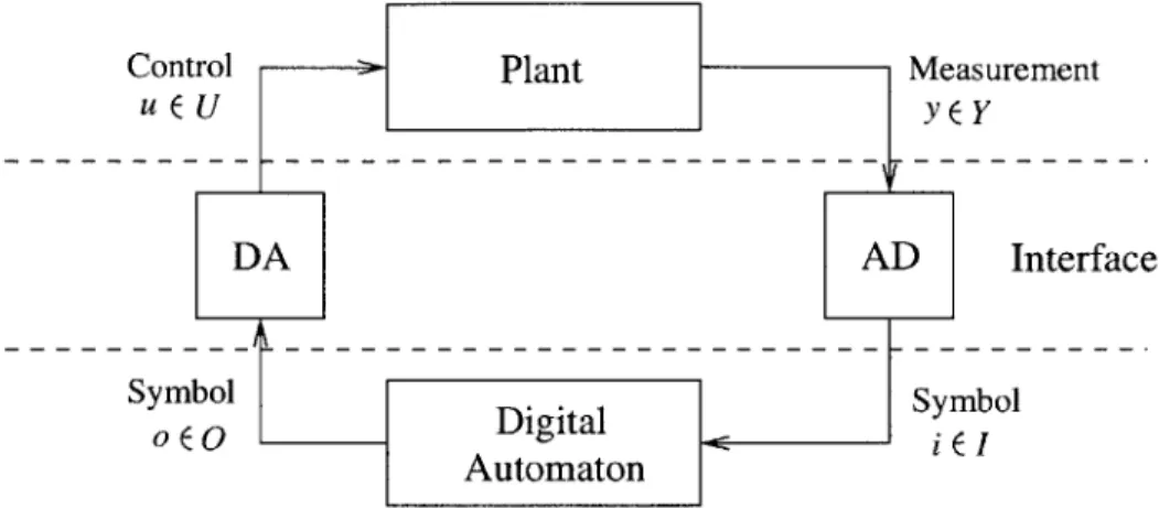
Reducing complexity was, and still is, an important reason for using hybrid models to represent the dynamic behavior of physical systems. In fact, many physical systems can be naturally represented as hybrid systems with very simple, but adequate for the tasks at hand, models of the complex physical phenomena. For example, a very well-known instance of a hybrid system is a sampled data system (see figure 1-1). Here, a continuous-time linear time-invariant plant described by differential equations (which involve continuous-valued variables that depend on continuous time) is controlled by a discrete-time linear time-invariant plant described by linear difference equations (which involve continuous-valued variables that depend on discrete time). A typical

(20)

application is a digital control system where a computer (evolving in discrete-time) controls a physical system (evolving in continuous-time).

Control >0

Plant

Measurement

u EU yY

DA AD Interface

Symbol .igt. Symbol

OEO ~ Automaton E

Figure 1-1: Sampled data system

Another familiar example of hybrid systems (of particular interest to us in this the-sis) are switching systems. Here, the dynamic behavior of interest can be adequately

described by a finite number of dynamical models that are typically sets of differen-tial or difference equations, together with a set of rules for switching among these models. A simple application of switching systems is the heating and cooling system of a house. The furnace (providing the heat) and the air conditioner (providing the cool), along with the heat flow characteristics of the house, form a continuous-time system which is to be controlled. The thermostat is a simple asynchronous discrete-event driven system which basically handles the symbols {hot, normal, cold}. The temperature of the room is translated into these representations in the thermostat and the thermostat's response is translated back to electrical currents, which control the furnace and the air conditioner.

For a broad review of hybrid phenomenon we refer to [12]. There, several models available in the literature are surveyed along with more examples and discussions on design and analysis issues.

1.4 Piecewise Linear Systems

As described above, switching systems are characterized by a finite number of dynam-ical models together with a set of rules for switching among these models. A class of switching systems we will be particularly interested in this thesis is piecewise linear

systems (PLS). PLS are characterized by having both the logic in the controller and

the nonlinearities in the system model (such as saturations, hysteresis, etc.) appear-ing as piecewise linear functions, with the system dynamics described by standard integration elements as with linear systems. Therefore, this model description causes a partitioning of the state space into cells. These cells have distinctive properties in that the dynamics within each cell are described by linear dynamic equations. The

(21)

boundaries of each cell are in effect switches between different linear systems. Those switches arise from the breakpoints in the piecewise linear functions of the model. As we will see in chapter 3, depending if the switching rule associated with the PLS has memory or not, the cells may or may not intersect each other.

The reason why we are interested in studying this class of systems is to capture discontinuity actions in the dynamics from either the controller or system nonlineari-ties. On one hand, a wide variety of physical systems are naturally modeled this way due to real-time changes in the plant dynamics. On the other hand, an engineer can introduce intentional nonlinearities to improve system performance, to effect econ-omy in component selection, or to simplify the dynamic equations of the system by working with sets of simpler equations (e.g., linear) and switch among these simpler models (in order to avoid dealing directly with a set of nonlinear equations). In the next two sections we will talk about these two types of occurrences along with some illustrative examples.

1.4.1 Modeling with Switches

There are numerous examples where a system changes its dynamic equations. For instance, this can happen due to hitting certain boundaries (like a ball hitting a wall) or due to certain control actions (like the space shuttle separating itself from the rockets during a launch). A model for such systems can be seen in figure 1-2. Here we have several models and a switch. The purpose of the switch is to decide at every instant of time which model better represents the physical system. This decision is based on all available information, which may include present and/or past values of the states.

Model 1

Model p Switch

Figure 1-2: Switching between different models

Next we have some examples where this model can be naturally used.

" Friction. Another simple example is the modeling of static friction [49]. If an engineer chooses, for example, the Coulomb model (see figure 1-3) to describe friction on a certain physical system, then the dynamics of the system switches (the friction force changes sign) every time the velocity changes sign. The Coulomb friction model is an ideal relay that will be discussed in more detail in chapter 5.

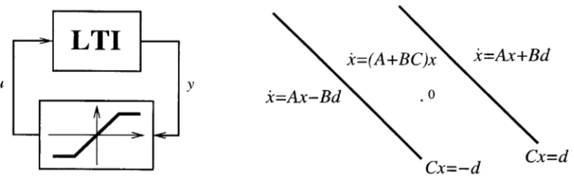
* Hysteresis. Many physical applications can be modeled as an LTI system in

feedback with an hysteresis (see figure 1-4). Such systems are similar to the ideal relay, like in the example of static friction, but with the difference that

(22)

F

Figure 1-3: Coulomb friction

the switches from "high" to "low" and from "low" to "high" do not occur at the same values of y. In other words, the hysteresis differs from the ideal relay in that it introduces memory into the nonlinearity. For instance, the single information that y(t) = 0 is not enough to decide on the value of u(t). This is determined not only by present values of y but also by past values of y. If

y(t) = 0 and if u(t - 0) = high then u(t) = high; otherwise, u(t) = low. Since

the switching rule has memory, the two cells, resulting from the two state space partitions, intersect each other in a region containing the origin. More details on hysteresis can be found in chapter 5.

L TI

U _y

Figure 1-4: Hysteresis

* Saturation. Every actuator in physical systems eventually saturates if the input

command exceeds certain levels. A very common model of a saturated actuator can be seen in figure 1-5. Here, y is the input to the actuator and u is the approximate input to the plant. Saturation systems will be studied in detail in chapter 7.

" Collisions. A system where its dynamics change as it hits certain boundaries is a simple ball in a room under gravity. A usual way of modeling such a system is to set instantaneously the velocity from v to -pv, where p E [0, 1] is the coefficient of restitution, when the ball hits the floor.

* Spring with damage protection. Consider a spring connected with a mass. In

order to protect the spring from over extension and avoid its damage, a "stop" device is placed at a desired position (see figure 1-6).

(23)

LTI

U _y Figure 1-5: Saturation Stop Spring Mass Force

Figure 1-6: Mass-spring with damage protection

Once the spring reaches the maximum allowed extension, the dynamics of the system change. We have then a different model depending if the spring protec-tion is touching the "stop" or not.

1.4.2 Control with Switches

It is well known that plant models are inherently inaccurate, and controllers regulat-ing processes described by such models must be able to ensure satisfactory closed-loop performance in the presence of exogenous process disturbances which cannot be mea-sured. Modern linear control theories (e.g., pole-placement/observer theory, linear quadratic theory, H, theory, and the like) are now very highly developed. Those the-ories can be used to design controllers with such capabilities for processes admitting linear models, providing the models uncertainties are time-invariant and "sufficiently small". However, for "large" model uncertainties derived from real-time changes in the plant dynamics, common sense suggests (and simple examples prove it) that no single, fixed-parameter linear controller can possibly regulate in a satisfactory way. This is the reason why control switching strategies like the ones in figures 1-7 and 1-8 must be used to control such systems.

Figure 1-7 shows a rather common approach in modeling and controlling physical phenomena. In this case, we have sets of simpler equations and we switch among these simpler models in order to avoid dealing directly with a set of nonlinear equations. A controller is then designed individually for each model and a switch decides at every instant of time which one to use.

(24)

Controller 1 Model 1

Controller p Model p Switch

Figure 1-7: Switching between different pairs of models/controllers

Controller 1 T

Model

Controller p Switch

Figure 1-8: Switching between different controllers

In some cases (see figure 1-8), one model together with several controllers may be enough (when compared with figure 1-7). Once again, a switch decides which controller to use at any given time.

Next we present some examples of control with switches.

" Inverted pendulum. In [4], an inverted pendulum is modeled and controlled differently in two distinct regions of the state space. The first objective is to bring the pendulum close to the upright position. Once there, a linearize model

and controller can be used to keep the pendulum in the upright position.

* Anti-lock brake system (ABS) for a car. The aim of the ABS is to improve the

effectiveness of a vehicle to brake by maintaining the tire braking torque at or near its maximum value. The key factor is the tire adhesion to the road as braking torque is applied. A typical torque curve can be seen in figure 1-9.

Tyre Adhesion

A B Wheel Slip

Figure 1-9: Typical tire adhesion curve for brake control

The tire adhesion is at its highest value between wheel slip A and B in figure 1-9. If wheel slip increases beyond B the wheel 'locks', tire adhesion decreases, and more importantly the driver looses the ability to steer the vehicle, i.e. the

(25)

system is considered unstable. The aim of the ABS controller is to keep wheel slip between A and B in the figure. A control strategy is proposed in [52]. There, a rule-based controller of ten rules was constructed resulting in something like 50 cells dividing the state-space.

e Hopping robots. More complex examples are hopping robots [53] or the dribbling of a basketball. In the case of the hopping robot, the boundary is the floor. As for the dribbling of a basketball, besides the floor, we have the hand of the player as another boundary (and also as the control). As they hit the floor

(and the hand in the case of the basketball), their dynamics change. These phenomena can be captured by PLS making the mathematical representation of their complicated dynamics simple.

Let's take the hopping robot, for instance. Consider a one legged robot (mono-pod) that hops (see figure 1-10). As described in [53], the hopping cycle is divided into three segments. Imagine we start when monopod touches the ground (figure 1-10.a). The spring will then begin to compress until this is fully compressed (figure 1-10.b). In this segment, gravity together with the leg spring, damping, and the controller determines the monopod's motion. These forces remain active during the second segment, except for the controller that switches sign in order to decompress the spring. This continues until the spring is completely decompressed (figure 1-10.c), indicating the end of the second seg-ment. The third and last segment of the cycle starts when the monopod leaves the floor. Here, gravity alone determines the monopod's motion. Eventually, it reaches its highest altitude (figure 1-10.d) and, finally, comes back to the ground (figure 1-10.a) where the cycle starts all over again.

a b c d

Figure 1-10: Different stages of a hopping monopod

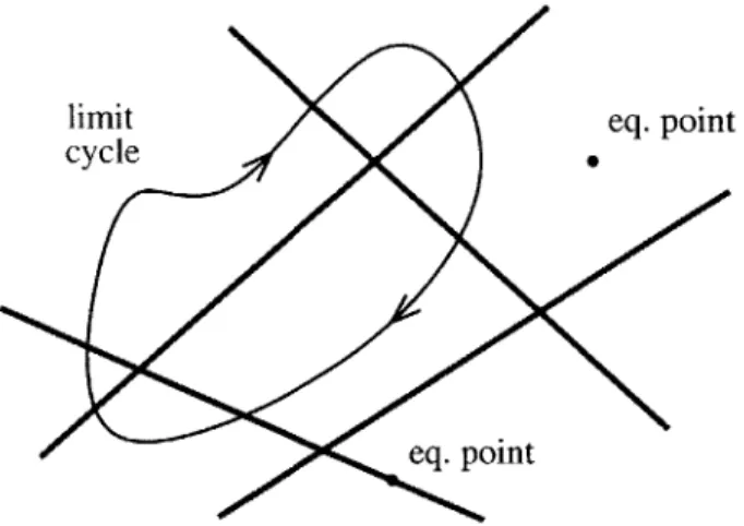
In general, a hopping robot is to follow a certain prescribed nominal trajectory. Since such nominal trajectory returns to its initial condition every cycle, we call these closed trajectories (see figure 1-11). The idea is to make sure the robot returns to this closed trajectory if, for some reason, it starts away from it, in a way that it does not fall over.

* Automatic tuning of PID regulators and delta-sigma modulators. An important

(26)

Initial condition

System 1

System 2

Figure 1-11: Closed trajectory switching among different systems

in many industrial controllers [6]. The basic idea behind this technique is to induce an oscillator (closed trajectory) by introducing an hysteresis in feedback with a stable open loop plant (see figure 1-4). Under certain assumptions, it is possible to determine several points on the Nyquist curve of the plant by measuring the frequency of the oscillation induced by the relay feedback. With this information, it is possible to calculate suitable parameters for simple controllers of the PID type.

Another application is the delta-sigma modulator as an alternative to conven-tional A/D converters [2]. Here, a relay is again used to produce a bit stream

output whose pulse density depends on the applied input signal amplitude.

1.5 Analysis of Piecewise Linear Systems

As seen before, sometimes it is natural and easy to model systems as a hybrid sys-tems. However, the same cannot be said about analyzing or designing controllers for these systems. In practice, the designer of hybrid systems is usually confronted with relations for which no general mathematical solutions exist. The problem is com-pounded by the peculiar behavior of hybrid systems: superposition no longer applies, the response of an hybrid system often depends on its initial state, and the nature of the system transient usually changes at different nominal operating points in the state space. For all these reasons, there does not exist a unified and generalized method of hybrid system analysis. In fact, the large diversity of hybrid systems suggests that, with a single design approach, most of the results would end up being unnecessarily

conservative. To deal with diverse hybrid systems we need to break this large class

of systems into several smaller classes. Each of these classes of hybrid systems should consist of systems that have certain properties in common. For instance, static sys-tems could be one class; or linear syssys-tems; or more complex ones like piecewise linear systems (PLS). Then, a comparable diversity of design and analysis tolls and proce-dures should be developed for each one of them. The goal of this thesis is to give a step forward in understanding and developing tools for a class of hybrid systems known as PLS.

(27)

1.5.1 Previous Results

Although widely used and intuitively simple, PLS are computationally hard and very few theoretical results are available to analyze most PLS. More precisely, one typically cannot assess a priori the guaranteed stability, robustness, and performance proper-ties of PLS designs. Rather, any such properproper-ties are inferred from extensive computer simulations. But, despite the lack of good theoretical analysis tools, PLS are used as an analysis and design methodology which is known to work in many engineering applications (like hopping robots, ABS, inverted pendulum, missile autopilots [13], robotic manipulators [14], autopilot of aircrafts [63]). However, in the absence of such analysis tools, these designs come with no guarantees. In other words, complete and systematic analysis and design methodologies have yet to emerge.

There are, however, some results for special classes of PLS. For instance, analysis in the phase plane of second-order systems has been studied for a while now. Early classical references discussing oscillations in mostly second-order systems using phase-plane analysis can be found in [1, 10, 29, 31, 60]. Other more recent references are [28, 36, 45, 46, 57]. Phase portrait analysis is a powerful graphical technique that presents global dynamic behavior for linear, piecewise linear, and even many nonlinear model descriptions. However, it is essentially restricted to models with two states only (or perhaps three states with todays computational graphic tools).

In [28], sketches of analysis and numerical simulations of a few model problems showed that "simple" differential equations of dimension three or greater can possess solutions of stunning complexity. Since such systems play an important role in the modeling, analysis, and design of nonlinear processes, an understanding of typical structures of their solutions is essential.

In the analysis of equilibrium points of PLS, recent results on the stability of equi-librium points for certain classes of PLS can be found in [34, 51, 30]. There, a search for piecewise quadratic Lyapunov functions is performed using convex optimization. Partitioning of the state-space is the key in this approach. For most PLS, construc-tion of piecewise quadratic Lyapunov funcconstruc-tions is only possible after a more refined partition of the state space, in addition to the already existent natural state space partition of the system. As a consequence, the analysis method is efficient only when the number of partitions required to prove stability is small. In chapter 4 we show that even for a simple second order system, the method can become computationally intractable. Also, the method does not scale well with the dimension of the system. For high-order systems, it is extremely hard to obtain a refinement of partitions in the state-space to efficiently analyze PLS. Another disadvantage of finding Lyapunov functions in the state space is that they are not capable of analyzing limit cycles.

Over many years, there has been extensive research on certain classes of PLS. Relay feedback systems (RFS) (a simple PLS that will be the topic of chapter 5) is one of these classes. Many results exist in the literature to analyze RFS. Research for this class of PLS was motivated by relays in electromechanical systems and simple models of dry friction (see the friction example in section 1.4.1). [8] and [64] are references that survey a number of analysis methods and results. Rigorous results for analysis

(28)

of local' stability of relay feedback systems can be found, for example, in [3, 33, 66]. In [23], reasonably large regions of stability around locally stable limit cycles were characterized. However, even for this simple class of PLS, very little is known about its global behavior. [60, 28] presents global analysis results for second order systems and [41] presents global stability results that can be applied to systems of order higher than two, including infinite-dimensional and uncertain systems. Unfortunately, many important relay feedback systems are not covered by this result.

Another class of PLS that has received great attention from researchers is sat-uration systems (see figure 1-5). The study of such systems is motivated by the possibility of actuator saturation or constraints on the actuators, reflected in bounds on available power supply or rate limits. These cannot be naturally dealt with within the context of standard (algebraic) linear control theory, but are ubiquitous in control applications. The fact that linear feedback laws when saturated can lead to instability has motived a large amount of research. The well known result which states that a controllable linear system is globally state feedback stabilizable, holds as long as the control does not saturate. In many applications, more often than not, the control is restricted to take values within certain bounds which may be met under closed-loop operation. Because feedback is cut, control saturation induces a nonlinear behavior on the closed-loop system. The problem of stabilizing linear systems with bounded controls has been studied extensively. See, for example, [59, 55, 62] and references therein.

Analysis of saturation systems (SAT) does not have such an extensive list of publications as synthesis. Some SAT can be analyzed by just using the circle or Popov criterion. Both of these criterion, however, are expected to be very conservative for systems of order greater than three. The Zames-Falb criterion [68] reduces the conservatism of both the circle and Popov criterion by taking in consideration the slope restrictions of the saturation. This method, however, is difficult to implement. Integral quadratic constraints (IQC) [35, 16, 44, 42] gives conditions in the form of LMIs that, when satisfied, guarantee stability of SAT. However, all of these analysis tools fail to analyze SAT with unstable nonlinearity sectors.

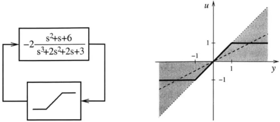
Example 1.1 Consider the SAT on the left of figure 1-12. If the saturation in the system is replaced by a linear constant gain of 1/2, the system becomes unstable (see the right side of figure 1-12). This means the system has an unstable nonlinearity sector. All the analysis tools described above fail to analyze systems with unstable nonlinearity sectors, like this one.

As we will see in chapter 7, the origin of this system is globally asymptotically

stable. 0

Other PLS, like on/off systems (see figure 1-13), can also be analyzed with the tools described above, basically with the same advantages and disadvantages as SAT.

On/off systems (OFS) system are characterized by an LTI system in feedback with

(29)

-2 s2+s+6 s3+2sk2s+3

Figure 1-12: 3d-order system with unstable nonlinearity sector

an on/off controller defined as

u(t) = max {0, y(t) - d}

LTI

-U _y

d

Figure 1-13: On/Off System

OFS can be found in many engineering applications. In electronic circuits, diodes

can be approximated by on/off controllers. Transient behavior of logical circuits that involve latches/flip-flops performing very fast on/off switching can be modeled using on/off circuits and saturations. In general, on/off circuits have many applications in electronics and circuit design. Another area of application of OFS is aircraft control. For instance, in [12], a max controller is designed to achieve good tracking of the pilot's input without violating safety margins.

1.5.2 Contributions

The fact that PLS must be studied as a whole is one of the reasons that makes this class of systems so hard to analyze. This is due to their hybrid nature. It is not enough, for instance, to study their subsystems separately. Even if each individual subsystem is stable, there is no guarantee that the PLS is also stable (see example 3.4). In practice, due to the unavailability of rigorous mathematical tools, exhaustive sim-ulation and/or experiment are, in most situations, the only alternatives to analyze most PLS.

(30)

The idea consists in finding quadratic Lyapunov functions on switching surfaces that can be used to prove that impact maps, i.e., maps from one switching surface to the next switching surface, are contracting in some sense. The search for surface quadratic Lyapunov functions is done by solving sets of linear matrix inequalities (LMIs) using efficient computational algorithms. Contractions of impact maps can then be used to conclude about global stability, robustness, and performance of PLS.

The novelty of this work comes from expressing impact maps induced by an LTI flow between two hyperplanes as linear transformations analytically parametrized by a scalar function of the state. Furthermore, level sets of this function are convex subsets of linear manifolds with dimension lower than that of the switching surfaces. This allows us to reduce the problem of finding quadratic surface Lyapunov functions to solving a set of LMIs, which can be efficiently done using available computational tools.

The main difference between this and previous work, e.g. [30, 34, 50], is that we look for quadratic Lyapunov functions on the switching surfaces instead of quadratic Lyapunov functions on the state space. An immediate advantage is that this allows us to analyze not only equilibrium points but also limit cycles. Another advantage is that, for a given class of PLS, complexity of analysis does not increase with the dimension of the system. Also, the analysis method proposed in [30, 34, 50] requires, in general, a further partition of the state space (besides the natural one imposed by the PLS). In our case, we only need the natural partitions imposed by the PLS. In chapter 4, we have an example of a second order system for which the number of partitions required in [30, 34, 50] is so high that it is computationally intractable. Quadratic surface Lyapunov functions, however, are easily found.

In the first part of this thesis, we will study global stability analysis of limit cycles and equilibrium points of PLS. We start with limit cycles. The study and under-standing of limit cycles are of great interest in many applications. Hopping robots are examples of such applications. Here, it is important to show a certain design control strategy of a hopping robot is globally stable in its domain of operation. This ensures that as long as the robot starts within its domain it will not fall and, more-over, it will converge asymptotically to its nominal trajectory. However, no results are available to prove such properties. Although many walking robots are known to walk, their stability and robustness have only been shown through exhaustive simulations and experiments. This is true, even for simple walking robots, like monopods. This, together with the fact that walking robots is a very active area of research, motivates the development of such analysis tools.

In general, there is little known about global stability of periodic solutions. In this thesis, we will first give existence and local stability results of periodic solutions of PLS, and then focus on global stability analysis. We start by analyzing a simple class of PLS known as relay feedback systems (RFS). One of the motivations to consider RFS first is that for symmetric unimodal limit cycles2, only a single impact map needs to be analyzed. Thus, this is a perfect class of systems to introduce global analysis using quadratic surface Lyapunov functions. The idea is to find a quadratic

2

Constructive global analysis of hybrid systems

Constructive Global Analysis of Hybrid Systems

by

Jorge Manuel Mendes Silva

Gongalves

Submitted to the Department of Electrical Engineering and Computer

Science

in partial fulfillment of the requirements for the degree of

Doctor of Philosophy

at the

MASSACHUSETTS INSTITUTE OF TECHNOLOGY

September 2000

©

Massachusetts Institute of Technology 2000. All rights reserved.

Author .

Depalment of Electrical Engineering and Computer Science

August 29, 2000

Certified by..

Al4

(7 .

Certified by...

.

Munther A. Dahleh

Professor

Thesis Supervisor

...

Associate Professor

- ---

In !-

i S

ervisor

Arthur C. Smith

Chairman, Department Committee on Graduate Students

OCT 2 3 2000

BARKER

Constructive Global Analysis of Hybrid Systems

by

Jorge Manuel Mendes Silva Gongalves

Abstract

Acknowledgments

Contents

List of Figures

List of Tables

Chapter 1

Introduction

1.1

Analysis of Feedback Systems

[53].

1.2

Nonlinear Systems

1.3

Hybrid Systems

Plant

1.4

Piecewise Linear Systems

1.4.1

Modeling with Switches

L TI

LTI

1.4.2

Control with Switches

1.5

Analysis of Piecewise Linear Systems

1.5.1

Previous Results

LTI

1.5.2

Contributions