Correlation Between the Precipitation and Energy Production at Hydropower Plants to Mitigate Flooding in the
Missouri River Basin By
Rachel Foley
Submitted to the
Department of Mechanical Engineering
in Partial Fulfillment of the Requirements for the Degree of Bachelor of Science in Mechanical Engineering
ARCHNES
MASSACHUSETTS INST Ef OF TCNLGJUL
3
2LRI
LIRAIES
at theMassachusetts Institute of Technology
June 2013
@ 2013 Rachel Foley. All rights reserved.
The author hereby grants to MIT permission to reproduce and to
distribute publicly paper and electronic copies of this thesis document in whole or in part in any medium now known or hereafter created.
Signature of Author:
Department of Mechanical Engineering May 10, 2013
Certified by:
"I
Accepted by:
Professor Anthony Patera Ford Professor of Engineering Thesis Supervisor
Anette Hosoi Professor of Mechanical Engineering Undergraduate Officer
Correlation Between the Precipitation and Energy Production at Hydropower Plants to Mitigate Flooding in the
Missouri River Basin by
Rachel Foley
Submitted to the Department of Mechanical Engineering on May 10, 2013 in Partial Fulfillment of the
Requirements for the Degree of Bachelor of Science in Mechanical Engineering
ABSTRACT
Currently, hydropower plants serve as one source of green energy for power companies. These plants are located in various geographical regions throughout the United States and can be split into three main classifications: run of river, basins, and reservoirs. The energy production at hydropower plants can vary on a monthly basis, and this change is recorded for company purposes. This study used data provided for five reservoir plants in the Missouri River Basin to model these variations, and determine a correlation between the precipitation and energy production. The parameters provided and modeled included the precipitation measured at each hydropower plant, the evaporation from the surface of the reservoir, the inflow into the reservoir, the outflow from each plant, the energy generation of each plant, and the reservoir elevation every month from June 1967 to December 2012. Using these monthly values, two separate models were created: a model that relates the power generation as determined from the energy production to the outflow and the effective hydraulic head at the hydropower plants, and a second model correlating the effective hydraulic head and the precipitation measured in the reservoir. The results showed that the energy production varied proportional
ly to the product of the monthly precipitation and outflow for each of the hydropower plants, up to the maximum installed capacity at each of the plants. Beyond this maximum installed power, there was no correlation between increased precipitation or outflow and the power produced.
Thesis Supervisor: Anthony Patera Title: Ford Professor of Engineering
TABLE OF CONTENTS Abstract 3 Acknowledgements 4 Table of Contents 5 List of Figures 6 List of Tables 7 1. Introduction 8
1.1 Hydrology in the Missouri River Basin 8
1.1.1 Flooding on the Missouri River 9
1.1.2 Dam Usage 9
1.2 Hydropower plants 9
1.2.1 Montana and North Dakota 10
1.2.2 South Dakota 10
2. Model Development 11
2.1 Correlation Between Precipitation and Energy Production 11
2.2 Production Correlation 12
2.2.1 Assumptions 13
2.2.2 MATLAB Modeling 14
2.3 Effective Hydraulic Head Correlation 14
2.3.1 Assumptions 16
2.3.2 MATLAB Modeling 16
3. Experimental Evaluation 17
3.1 Robustness of Models 17
3.2 Theoretical Relationship Between Precipitation and Energy Production 17 3.3 Experimental Relationship Between Precipitation and Energy Production 17
4. Results and Conclusion 18
5. Bibliography 23
6. Appendices 24
Appendix A. Production Correlation MATLAB code 24
Figure 1-1:
Figure 1-2:
Figure 2-1:
Figure 2-2:
Figure 2-3:
Figure 2-4:
Figure 2-5:
Figure 4-1:
Figure 4-2:
Figure 4-3:
Figure 4-4:
LIST OF FIGURESMap of the Missouri River and Tributaries Diagram of a Reservoir Hydropower Plant
Block Diagram of Systems Used in Modeling Hydropower Plants
Fort Peck Average Monthly Energy Generation from 1967 - 2012
Fort Peck Average Monthly Outflow in 1,000 Acre-feet from 1967 - 2012
Average End-of-Month Reservoir Elevation at the Fort Peck Dam
Average Monthly Precipitation at the Fort Peck Dam
Garrison: Correlation Between Power, Head, and Outflow Monthly Power vs. (Outflow* Effective Hydraulic Head)
Garrison: Correlation Between Elevation, Precipitation, and Flow
Actual Change in Elevation vs. Theoretical Change in Elevation
8 9 11 12 12 15 15 18 19 20 21
LIST OF TABLES
Table 2-1: Comparison of similar outflow values at the Oahe hydropower plant 13
Table 4-1: Production Correlation Coefficients 19
1.
Introduction
In the upper Midwest, the flow of water is an absolute necessity. The semi-arid region is home to over twelve million people and much of the land outside the major cities is devoted to farming. As such, it is important to monitor the hydrology of the Missouri River Basin, which is the main supply of water for the region. Beyond tracking the rainfall and snowfall in the region, the usage of dams is necessary to control the level of the river and reduce the effects of the large amounts of precipitation during the spring months, namely flooding, as well as provide another source of electricity for the company operating the dam.
1.1 Hydrology in the Missouri River Basin
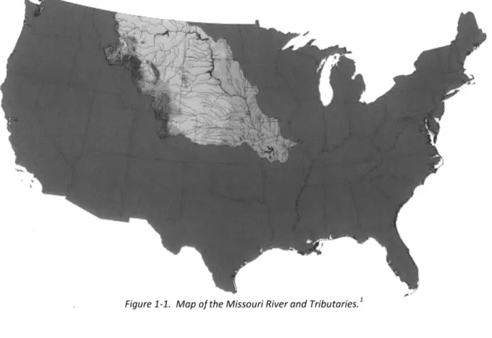
The Missouri River Basin covers a span of approximately 530,000 square miles over nine states in the upper Midwest, including Montana, Wyoming, Colorado, North Dakota, South Dakota, Nebraska, Kansas, Minnesota, Iowa, and Missouri. The 170,000 square miles of farmland contained within the basin constitutes approximately one-fourth of the total farmland in the United States. With
approximately 2,500 tributaries and stretching for 2,341 miles, the Missouri River constitutes one of the most important waterways for the Midwest.
Figure 1-1. Map of the Missouri River and Tributaries.'
1.1.1 Flooding on the Missouri River
It can also pose a great threat to the agricultural industry during late spring, as the rainfall increases and couples with runoff in the Rockies to increase the depth of the river. This increase in river depth has severe long-term effects, including lengthy flooding seasons and destruction of crops and property where the water level rises above the banks.
The basin experiences an average of 8 to 10 inches of rain, though most of the precipitation comes in the form of snowfall during the winter months.2
It is because of this rainfall and snowfall that severe flooding occurs, such as the flooding in Iowa during the summer of 2011.
1.1.2 Dam Usage
In order to combat this flooding, dams have been built along the length of the Missouri River. Dams are found downstream of large lakes, which constitute the reservoirs that water can be drawn from or stored as precipitation varies. The intent of the dams is to allow for regulation of the river depths on either side of the dam, and in series, they can potentially eliminate flooding in the Missouri River Basin.
Unfortunately, due to thunderstorms that bring heavy rainfalls, this is not always possible. When large rainfalls occur over the course of many months, the dams are used to mitigate flooding by releasing increased amounts of water in areas most affected by the rain.
1.2 Hydropower Plants
Dams are often coupled with hydropower plants so that the regulation of water levels can be used effectively to also produce electricity for the surrounding area. As water passes through the dam, the flow causes turbines within the dam to spin, which combine with a generator to create electricity. The
hydropower plants found in dams are considered reservoir plants, one of the three major types of hydropower plants used in the United States today.
Figure 1-2. Diagram of a reservoir hydropower plant.'
2 "Missouri River Mainstem Reservoir System Master Water Control Manual". U.S. Army Corps of Engineers.
The hydropower plants found on the Missouri River are located in Montana, North Dakota, and South Dakota. These plants include Fort Peck, Garrison, Gavins Point, Big Bend, Fort Randall, and Oahe, all of which are operated and monitored by the US Army Corp of Engineers. Due to lack of precipitation records, Big Bend will not be included in this study. For the purpose of this study, it is also assumed that these plants are operational for 12 hours every day. This is the assumption because hydropower plants can either be baseload or peaking power plants, meaning that the plant either provides a lower steady amount of power for the company or it peaks in production during the parts of the day when more electricity is being used, respectively.
1.2.1 Hydropower Plants in Montana and North Dakota
Two of the reservoir plants along the Missouri River are located in Montana and North Dakota: Fort Peck and Garrison. The Fort Peck dam is the first of the series of dams along the Missouri River. The dam forms Fort Peck Lake, which has a surface area of 383 square miles. The hydropower plant itself
has a hydraulic head of 220 feet, and an installed capacity of 185 MW.
The Garrison dam is the second dam in the series, and is located in central North Dakota on Lake Sakakawea. The lake has a surface area of 597 square miles, making it the largest of the reservoirs
included in this study. The Garrison dam is fifth-largest earthen dam in the world, and the hydropower plant has an installed capacity of just over 583 MW.
1.2.2 Hydropower Plants in South Dakota
The other three hydropower plants included in this study are Oahe, Fort Randall, and Gavins Point. These plants are located in central and southern South Dakota, and constitute 1238 MW of power generation capacity. The Oahe dam is third in the series of dams, and creates the second largest
reservoir of the set of dams. Lake Oahe has a surface area of 578 square miles and a capacity of just over one trillion cubic feet. The Oahe hydropower plant has the largest installed capacity at 786 MW and generates over 2,500 GWh of energy yearly.
Fort Randall, situated near Pickstown, South Dakota, is the fifth dam in the series along the Missouri River. The reservoir created, Lake Francis Case, has a surface area of 159 square miles. The Fort Randall hydropower plant has an installed capacity of 320 MW.
Finally, Gavins Point dam is the final dam of the series and is located along the South Dakota-Nebraska border. The Lewis and Clark Lake is created from the dam, and has the smallest surface area at just 49 square miles. The Gavins Point hydropower plant also has the lowest installed capacity: 132 MW.
2.
Model Development
Development of model to correlate the precipitation and production at hydropower plants can have an extremely important impact on how hydropower plants are run. Most ideally, the model developed
by this study could help to anticipate and mitigate the effects of large rainfalls in the Missouri River basin. As a consequence, the power produced could become the primary indicator for determining how much outflow the plant is seeing, and how much more (or less) it should be seeing in order to prepare for the expected average rainfalls and any larger or smaller amounts of forecasted rain.
2.1 Correlation Between Precipitation and Energy Production
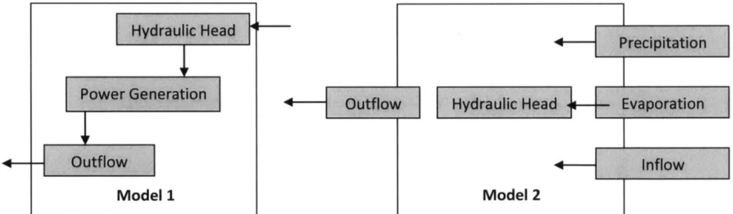
In order to approach this problem, the provided information from each of the five plants was broken down into two separate, but related models. The first model, hereafter to be described as the
Production Correlation, analyzed the relationship between the outflow, effective hydraulic head, and the power production at the five plants. The second model, hereafter to be described as the Effective
Hydraulic Head Correlation, analyzed the relationship between the inflow, outflow, precipitation, evaporation, and effective hydraulic head in the reservoir itself.
By creating two separate models, the problem of creating correlations between each of these parameters was simplified and allowed for less complexity in the overall model. The first model worked to describe what happened inside the power plant, while the second allowed for the reservoir to be an
isolated system. Taken together, they effectively describe how the precipitation correlates to the production inside a hydropower plant.
Model 1 Model 2
Figure 2-1. Block diagram of the information used to obtain the two models used in this study. The flow into and out of the system describes the use of each particular set of values in creating the models.
The technical data provided for each of the plants analyzed in this study is available on the US Army Corp of Engineers website, and the precipitation measurements were made available by the NOAA. This information was the only information used in creating the models necessary for this study, but each was manipulated to increase the ease of use during the course of the study. All manipulated information will be discussed in the section that it was used in the following model development discussion.
2.2 Production Correlation
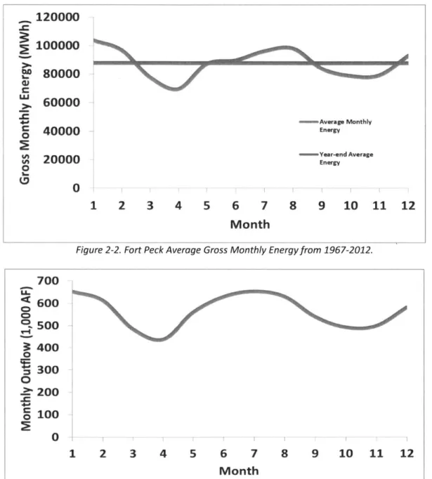
In order to create the Production Correlation, the information for each plant used included the energy production, the effective hydraulic head, and the outflow from the dam. As can be seen in Figures 2-2 and 2-3, the general shape of the average values for average gross monthly energy produced and the average monthly outflow at the Fort Peck hydropower plant are highly correlated. However, when broken down by year, the outflow in and of itself is much less likely to precisely predict the fluctuations in the gross monthly energy production. This trend can be observed for months with
identical outflows and varying production values. Table 2-1 demonstrates an example of this at the Oahe Dam. Similar results are found with each of the other power plants used in this study. As such, it was important for this study to understand the cause behind the unexpected fluctuations at the plants.
Figure 2-2. Fort Peck Average Gross Monthly Energy from 1967-2012.
1 2 3 4 5 6 7 8 9 10 11 12
Month
Figure 2-3. Fort Peck Average Monthly Outflow in 1,000 Acre-feet from 1967-2012.
120000
100000
V
80000
a,
60000
S40000
Eeg #A20000
Eeg0
0
Average Monthly Energy 1 2 3 4 5 6 7 8 9 10 11 12Month
700
L&600
0 500 9 400 0 = 3000
200 8 1000
AOTable 2-1. Comparison of similar outflow values at the Oahe hydropower plant.
Month Year Energy (MWh) Outflow (1,000 AF) Head (ftmsl)
Oct 2005 58719 479 1573.9 Sep 2007 61343 479 1580.9 Dec 1977 169675 1143 1594.8 Jan 1978 172574 1143 1596.9 Dec 1974 178611 1143 1605.1 Feb 1973 198373 1312 1603.1 Dec 1999 204235 1312 1606.9 Feb 1998 218314 1312 1608.4 Jun 1986 222693 1312 1617 Dec 1999 204235 1747 1606.9 May 1975 285297 1747 1612.9
The first necessary manipulation of values in this study was the conversion of the energy production in MWh to power production in MW, then again to (Ibs*ft2
/s3
). Because there is no direct conversion between the energy and power production without the time over which the energy was produced, this study assumed that each plant would be operational for approximately 12 hours every day. This assumption was made because of the nature of the plants as both baseload and peaking power plants, as discussed in the Introduction of this paper.
The second necessary manipulation of values was the conversion of outflow to (ft3
). This particular conversion was merely a scaling of the already acquired outflow values, and thus did not require any assumptions in this study. It may be noted that the correlations determined in this study are equivalent to correlations of the raw data itself. However, it was felt that consistency in units would ensure a more accurate conclusion drawn from the results. Assumptions made are discussed in the following section.
2.2.1 Assumptions
The first assumption made in beginning the creation of the model was that the correlation between the power production, effective hydraulic head, and outflow could be modeled as a simple linear regression. In assuming simplicity of the model, the correlations were more easily analyzed, and the relationship between the values was more accurately understood. The linear regression performed in
MATLAB was also double checked using the corrcoef function, ensuring that the model would
accurately predict any new values added to the system, and would provide a linear correlation between the three variables. This corrcoef function is defined by Equation 2-1, where R(ij) is a two-by-two
matrix of coefficients relating the product of the outflow and the effective hydraulic head and C(i,j) is the covariance matrix, which calculates how much these two variables change together.
R(i,
j)
= )C iicl(j,
j)
(2-1)The second assumption made was that the effective hydraulic head was equivalent (minus a scaling factor) to the reservoir elevation provided for each of the plants. Because the hydraulic head is
elevation from month to month is proportional to the change in hydraulic head, thus the reservoir elevation was used due to not having the monthly hydraulic head measurement available for this study.
The third assumption of the model was that, should the power generation be dependent on any other outside factors, such as operator error or decreased generator efficiency, these effects were negligible for the scope of this project. As such, the model was created using only the outflow and effective hydraulic head. This also allows the model to recognize disparities in the power production at hydropower plants so that the effects of the said disparities can be discovered and corrected in a timely manner.
2.2.2 MATLAB Modeling
MATLAB was the primary source of modeling in this study. By using the MATLAB built in functions for linear regression models, the data provided for the five power plants in this study was compared with the theoretical regression model developed using the outflow and effective hydraulic head. This theoretical regression model utilizes a vector of regression coefficients to model the correlation between the variables. In order to fully understand the relationship between the different parameters analyzed for this model, the regression model included the outflow, the effective hydraulic head, and the product of the outflow and effective hydraulic head. This method is also effective by using a
minimum residual approach that compares the product of one of the variables and the beta values with the power vectors.
Using a three-dimensional scatter plot, the power generation data was plotted against the outflow and effective hydraulic head, while a mesh was developed from the minimum and maximum values of the outflow and effective hydraulic head. The gradient of the mesh was observed and noted for further
experimentations with each of the plants. The model took into account a single month over the course of 45 years for each of the plants, except Gavins Point where precipitation data was not available for the past 15 years the plant has been in operation.
The results of the MATLAB modeling are discussed in the Results and Conclusions section, and the MATLAB code used to model the Production can be found in Appendix A.
2.3 Effective Hydraulic Head Correlation
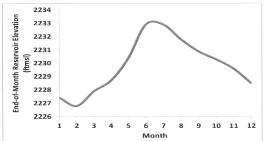
In order to create the Effective Hydraulic Head Correlation, the information for each plant used included the inflow into the reservoir, the precipitation and evaporation from the reservoir's surface, the outflow from the dam, and the change in reservoir elevation from month to month. As can be seen
in Figures 2-4 and 2-5, the general shape of the average values for average end-of-month reservoir elevation and the average monthly precipitation at the Fort Peck hydropower plant are moderately correlated. However, when broken down by year, the amount of precipitation at the plants in this study
is unlikely to accurately predict the variations in reservoir elevation. Similar results are found with each of the other power plants used in this study. As such, it was important for this study to understand the cause behind the variations in reservoir elevations.
2234 C 0 - 2233 mi 2232 2231 E 2230 2229 2228 0 -6 2227 2226 1 2 3 4 5 6 7 8 9 10 11 12 Month
Figure 2-4. Average End-of-Month Reservoir Elevation in feet mean sea level at the Fort Peck Dam.
2.5 C 0.5 0 1 2 3 4 5 6 7 8 9 10 11 12 Month
Figure 2-5. Average Monthly Precipitation in inches at the Fort Peck Dam.
The first necessary manipulation of values in this study was the conversion of the inflow and outflow of water in the reservoir from cubic feet to feet. This was done by using the provided values (in 1,000 AF) and dividing the inflow and outflow by the total surface acreage of the reservoir. This allowed for a direct correlation to be found between the movement of water through the reservoir with its changing elevation.
The second necessary manipulation of values was the conversion of evaporation from acre-feet to inches. This was done in a similar fashion to that of the inflow and outflow of water in the reservoir. By knowing the approximate surface area of the reservoir, the effective depth of evaporation could be obtained. This also allowed for a direct correlation between how much water is lost to the atmosphere
and the changing reservoir elevation.
The final manipulation was for that of the reservoir elevations themselves. Because the inflow, outflow, evaporation, and precipitation constitute changes in depth of the reservoir, the most useful form of the reservoir elevation was as a change in elevation from month to month. This allowed for the calculation of the "theoretical" depth change and its comparison to the actual depth change observed in the reservoir.
2.3.1 Assumptions
The first assumption made in beginning the creation of the model was that the correlation between the outflow, inflow, precipitation, evaporation, and effective hydraulic head could be modeled as a linear regression. The simplicity of the model assumed allowed for the correlations to be more easily analyzed, and the relationship between the values to be more accurately understood. The linear regression performed in MATLAB was also double checked using the corrcoef function, ensuring that the model would accurately predict any new values added to the system, and would provide a linear correlation between the variables used in this model. The function is used in the same manner as that function used in the production correlation discussed in Section 2.2.1.
The second assumption made was that the any runoff that occurred upriver from the hydropower plant was either negligible or included in the inflow values. Since the runoff would contribute to variations in the inflow values upriver, it is reasonable to assume that the inflow could account for most of the runoff experienced. Beyond this, the runoff experienced at the hydropower plant itself was excluded from the calculations. Any fluctuations that do not fit the model may be caused by this runoff, but these fluctuations are not contained within the scope this study.
The third assumption of the model was that, should the effective hydraulic head be dependent on any other outside factors, these effects were negligible for the scope of this project. As such, the model was created using only the previously mentioned parameters. This also allows the model to recognize disparities in the effective hydraulic head at hydropower plants so that the effects of the said disparities can be discovered and corrected in a timely manner.
2.3.2 MATLAB Modeling
MATLAB was the primary source of modeling in this study. By using the MATLAB built in functions for linear regression models, the data provided for the five power plants in this study was compared with the theoretical regression model developed using the difference between inflow and outflow and the difference between the precipitation and evaporation. This theoretical regression model utilizes a vector of regression coefficients similar to the production coefficients to model the correlation between these variables. In order to fully understand the relationship between the different parameters
analyzed for this model, the regression model included the aforementioned differences in flow and precipitation and evaporation levels. This method is also effective by using a minimum residual approach that compares the product of one of the variables tested and the beta values with the effective hydraulic head vectors.
Using a three-dimensional scatter plot, the change in reservoir elevation data was plotted against the differences, while a mesh was developed from the minimum and maximum values of the difference in inflow and outflow, as well as the difference in precipitation and evaporation. The gradient of the mesh was observed and noted for further experimentations with each of the plants. The model took into account a single month over the course of 45 years for each of the plants, except Gavins Point where precipitation data was not available for the past 15 years the plant has been in operation.
The results of the MATLAB modeling are discussed in the Results and Conclusions section, and the MATLAB code used to model the Effective Hydraulic Head can be found in Appendix B.
3.
Experimental Evaluation
3.1 Robustness of the Model
The model was tested with multiple plants with different capacities, varying reservoir levels, and differing precipitation values over the course of the time studied. In doing this, the study created a more robust model that has a greater probability of withstanding rigorous testing with other reservoir hydropower plants around the United States. By understanding the trends of the past 45 years, the model helps to create a baseline of what to expect on a yearly basis with power production and rainfall. The creation of a robust model also allows for more accurate predictions of the effects of high or low
rainfalls, and high or low production levels. This, in turn, gives rise to a more accurate methodology for monitoring the rise and fall of the reservoir and mitigating flooding during high rainfall months.
Further experimentation following this study could be conducted using information from plants not located in the same geographical region to ensure the model is complete. This would create an even more robust model, and this could revolutionize hydropower production and how it relates to flooding throughout the United States.
3.2 Theoretical Relationship Between Precipitation and Production
The expectation of this study was that the precipitation and power production could be modeled in a single linear regression in order to make better use of the current information already obtained about the correlations from previous years. By using the MATLAB models discussed above, two separate
correlations made and combined to create a final model.
Since the power generated at a hydropower plant is proportional to product of the outflow and the effective hydraulic head, this shows how the precipitation creates changes in the power. Also, since we know that the effective hydraulic head is proportional to the change in flow over the area, plus
precipitation, minus the evaporation, the two models can be combined to create a final relationship:
P(MW) [is proportional to] Outflow*((Inflow-Outflow)/Area +Precipitation - Evaporation)
3.3 Experimentally Determined Relationship
This relationship can then be used to experimentally model the correlation between the
precipitation and power generation using real world data. It is important that the information collected from the power plants in the Missouri River basin be tested by this model and a regression model to ensure that the data being analyzed is not an edge case where most data wouldn't fit the model. The experimentally determined relationship between the precipitation and production at the hydropower plants in this study were determined with the aforementioned data, and are discussed in the Results and Conclusion section.
4.
Results and Conclusion
Two models were created to correlate the precipitation experienced at five hydropower plants in the Missouri River basin. The first was a model between the power and the product of the outflow and effective hydraulic head. The second modeled the relationship between the effective hydraulic head and four other factors: the inflow, outflow, precipitation, evaporation at each of the hydropower plants. These two models, when observed and analyzed together, show a strong correlation between the precipitation and power production at the five hydropower plants utilized during this study. However, beyond the installed capacity of the hydropower plants, there is no correlation between the
precipitation, outflow, and power production. This is understandable because even as you increase the volume of water, the generator can only produce up to its rated capacity.
Production correlation
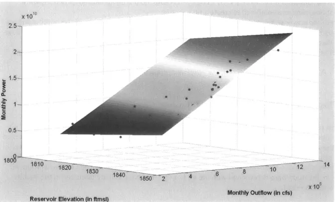
The production model for Fort Peck, Fort Randall, Gavins Point, Garrison, and Oahe provided invaluable information about the correlation between the power and the reservoir elevation. As discussed in Section 2.2, the Outflow in and of itself could not predict with complete accuracy the value of power production for that month. As suggested in Table 1, the effective hydraulic head also causes the power production to vary. Figure 4-1 shows that the power increases, as expected, with the product
of the outflow and effective hydraulic head since the gradient of the fitted mesh also follows this product. Similar plots were made for each month at each of the five power plants, and yielded results similar to that of Garrison.
**
10
X110
18081830 14 6 8 10 12 4
1850 2
Monthly Outflow (in cs) Reservoir Elevation (In ftmsl)
Figure 4-1. Correlation between the Monthly Power (in lbs*ft2/s), Effective Hydraulic Head (Reservoir Elevation in
ftmsl), and the Monthly Outflow (in cfs) at the Garrison hydropower plant. As the gradient suggests, the product of the latter two parameters is proportional to the power produced.
One final plot to compare the Power directly with the product of the outflow and effective hydraulic head was made to ensure the robustness of the model. This plot can be seen in Figure 4-2. As seen in this figure, and discussed previously, the power varies linearly with the product of the outflow and hydraulic head up to installed capacity at the power plant. Once the power has reached this maximum, there is no increase in power production. This occurrence can be seen in the plot as the small upward trends at intervals along the x-axis. The plants with a larger installed capacity exhibit these upward trends at a greater effective hydraulic head and outflow due to the ability for the plant to utilize greater volumes of water in production.
x 10 3.5-0.5 3e ri2.5 0 0Of .* ** g*r
~1.5
0 '0.5, 0.5 1 1.5 2 2.5Figure 4-2. Plot of the Monthly Power (in lbs*ft2
/sj) against the product of the Outflow (in cfs) and the Effective Hydraulic Head (Reservoir Elevation in ft) for allfive hydropower plants used in this study.
To support this model, the correlation coefficients as described in Section 2.2.1 were calculated for all five hydropower plants. The coefficients can be seen in Table 4-1. These coefficients reinforce the results in Figures 4-1 and 4-2, and suggest that this model could be applied to other hydropower plants with approximately 70% accuracy or greater. This also implies that it is feasible to apply this model to these hydropower plants to mitigate flooding along the Missouri River.
Table 4-1. Production Correlation Coefficients for each of the five hydropower plants analyzed in this study. The high correlation coefficients indicate a strong correlation between the power and the product of the outflow and effective hydraulic head.
Fort Peck Fort Randall Gavins Point Garrison Oahe Correlation Coefficient .8176 .9406 .8414 .6928 .9868
Effective Hydraulic Head Correlation
The effective hydraulic head model for Fort Peck, Fort Randall, Gavins Point, Garrison, and Oahe provided a highly accurate and robust correlation between the effective hydraulic head and the
precipitation. As discussed in Section 2.3, though precipitation and the reservoir elevation are somewhat correlated, alone precipitation can't explain the variations in reservoir elevation and thus effective hydraulic head. At the Garrison hydropower plant, the change in elevation seems to be uncorrelated with only the change in flow or the precipitation and evaporation. However, taken
together, the change in elevation can be fitted quite effectively to the theoretical change in elevation (as calculated by adding the change in flow over area and the difference between precipitation and
evaporation). The results found for Garrison are similar to those found at the other power plants involved in this study. Figure 4-3 shows these results.
0
1
~
-1.5-0.05 -2.5 -2
Monthly Precipitation -Evaporation (feet) Monthly Flow (feet)
Figure 4-3. Correlation between the Change
in
Elevation, Monthly Precipitation-Evaporation, and the Monthly Flowat the Garrison hydropower plant. The change
in
elevationis
directly proportional to the sum of the monthlyflow
and the monthly precipitation-evaporation.
The plot in Figure 4-4 compares this actual change in elevation (as taken from the difference between reservoir elevations from month to month) directly with the theoretical change in elevation calculated from the outflow, inflow, precipitation, and evaporation to ensure the robustness of the model. As seen in this figure, and discussed previously, there is a significant linear correlation between these values, showing that the model is indeed robust. This correlation remains constant for any change in elevation. However, if further studies of flood stage waters were to be conducted, it is likely that beyond flood stages the correlation would not exist. This is because the reservoir can only hold a certain volume of water, and beyond this, extra inflow or rainfall would only increase the amount of water being omitted from the reservoir, not to the reservoir itself.
20 r 15 . 10 10 IE 0 --15 0 10 15 20
Actual Change In Elevation (feet)
Figure 4-4. Plot of the Actual Change in Elevation against the Theoretical Change in Elevation. Allfive of the plants exhibit the same trend, which suggests that this model could be accurate for a wide range of hydropower plants.
As with the power production, correlation coefficients for Fort Peck described in Section 2.3.1, Fort Randall, Gavins Point, Garrison, and Oahe were calculated to support the findings of the model. The coefficients can be seen in Table 4-2. These coefficients reinforce the results in Figures 4-3 and 4-4, and suggest that this model could be applied to other hydropower plants with approximately 98% accuracy or greater. This also implies that it is feasible, when combined with the production model, to apply this
model to these hydropower plants to mitigate flooding along the Missouri River.
Table 4-2. Effective Hydraulic Head Correlation Coefficients for each of the five hydropower plants analyzed in this study. The high correlation coefficients indicate a strong correlation between the effective hydraulic head, outflow, inflow, precipitation, and evaporation at the plants.
Fort Peck Fort Randall Gavins Point Garrison Oahe
Correlation Coefficient .9902 .9842 .9850 .9872 .9869
Future Research
One of the most important points of future research would be to control the variations in the variables in this study. This control would allow for a reevaluation of the model to ensure the noise does not have any significance not covered by the scope of this model. Though the overall model created in this study provides an accurate picture of the correlation between precipitation and power
production at a hydropower plant, there is still room for further research. A more complex model could be created to account for the different geographical regions with hydropower plants in the United States. This would allow for use of the model in varying hydrological areas. Beyond this, a more
detailed account of the daily values of precipitation and production at the hydropower plants could lead to a model that could decrease the likelihood of flooding down river from the plants. Knowing how daily
for even higher precision when determining how much outflow is needed to prepare for high or low amounts of rainfall in a short amount of time.
5.
Bibliography
Monthly Project Statistics for Fort Peck, 2013-04-30 [Computer file]. Conducted by US Army Corp of Engineers. Accessed 2013-05-01. http://www.nwd-mr.usace.army.mil/rcc/projdata/ftpk.pdf
Monthly Project Statistics for Fort Randall, 2013-04-30 [Computer file]. Conducted by US Army Corp of Engineers. Accessed 2013-05-01. http://www.nwd-mr.usace.army.mil/rcc/projdata/ftra.pdf
Monthly Project Statistics for Gavins Point, 2013-04-30 [Computer file]. Conducted by US Army Corp of Engineers. Accessed 2013-05-01. http://www.nwd-mr.usace.army.mil/rcc/projdata/gapt.pdf
Monthly Project Statistics for Garrison, 2013-04-30 [Computer file]. Conducted by US Army Corp of Engineers. Accessed 2013-05-01. http://www.nwd-mr.usace.army.mil/rcc/projdata/garr.pdf
Monthly Project Statistics for Oahe, 2013-04-30 [Computer file]. Conducted by US Army Corp of Engineers. Accessed 2013-05-01. http://www.nwd-mr.usace.army.mil/rcc/projdata/oahe.pdf
Custom Monthly Statistics for Fort Peck, 1967-2013 [Computer file]. Conducted by the National Oceanic and Atmospheric Administration. Accessed 2013-03-01.
http://www.wrcc.dri.edu/cgi-bin/cli MAIN.pl?mt3176
Custom Monthly Statistics for Fort Randall, 1967-2013 [Computer file]. Conducted by the National Oceanic and Atmospheric Administration. Accessed 2013-03-01. http://www.wrcc.dri.edu/cgi-bin/cliMAIN.pl?sd6574
Custom Monthly Statistics for Gavins Point, 1967-2013 [Computer file]. Conducted by the National Oceanic and Atmospheric Administration. Accessed 2013-03-01. http://www.wrcc.dri.edu/cgi-bin/cli MAIN.pl?ne3165
Custom Monthly Statistics for Garrison, 1967-2013 [Computer file]. Conducted by the National Oceanic and Atmospheric Administration. Accessed 2013-03-01.
http://www.wrcc.dri.edu/cgi-bin/cli MAI N.pl?nd3376
Custom Monthly Statistics for Oahe, 1967-2013 [Computer file]. Conducted by the National Oceanic and Atmospheric Administration. Accessed 2013-03-01. http://www.wrcc.dri.edu/cgi-bin/cliMAIN.pl?sd6170
6.
Appendices
Appendix A: Production Correlation MATLAB Code
The code used to create the Production Correlation for each plant is sectioned by month. Because of the length of the code, only the month of January is included here. The code for February through December can be obtained by substituting that month for 'January' in the vector names.
X Jan FTPK = [ones(size(FTPK ReservoirElevation(:,l))) FTPKReservoirElevation(:,1).*FTPKOutflow incfs(:,l)...
FTPKReservoir Elevation(:,l) FTPKOutflowincfs(:,l)];
FTPK(:,1) = regress(FTPKPower(:,1), XJan FTPK);
figure
set(gca, 'FonLSI ze' , 16, FontIeig ', bold')
scatter3(FTPKReservoirElevation(:,l), FTPKOutflowincfs(:,1),... FTPKPower (:1 ' 1 cild');
hold
xlfit =
min(FTPK Reservoir Elevation(:,l)):.05:max(FTPK ReservoirElevation(:,l)); x2fit = min(FTPKOutflowincfs(:,l)):1000:max(FTPKOutflowincfs(:,l));
[X1FIT,X2FIT] = meshgrid(xlfit,x2fit);
YFIT = FTPK(1,1) + FTPK(2,1)*X1FIT.*X2FIT + FTPK(3,1)*XlFIT +
FTPK(4, 1) *X2FIT;
mesh (X1FIT, X2FIT, YFIT)
title (' J n inrre a iCn', 'e tint.iz', 16, ' Fontweight', bold
xlabel (' ev 1 ir E cao lu In (i Frt ) ', 'Fotu ize , 16, 'FontWoight', bold'
ylabel ( 'Mio nh u tuPoo Itis) (Wn tSu1', , 'F.ont. 16, ' Font .. iht ', 'tbold,') zlabel( 'Morthy 10 werc (MWV) ', tcurntSize'c, 16, ' Fcntigh qt ', 'hot dI') view(50, 10)
XJanFTRA = [ones(size(FTRAReservoirElevation(:,l)))
FTRAReservoirElevation(:,l).*FTRAOutflowincfs(:,1)... FTRAReservoirElevation(:,1) FTRAOutflowincfs(:,1)]; FTRA (: , 1) = regress-(FTRAPower (:,1), XJanFTRA);
figure
set (gca, ' .nt i ', 16, 'Font e i ht ' , ' old ' )
scatter3(FTRAReservoirElevation(:,1), FTRAOutflow incfs(:,1),... FTRAPower (:,1) , ' 1!led' ;
hold an xlfit =
min(FTRAReservoir Elevation(:,1)):.05:max(FTRA_ReservoirElevation(:,1));
x2fit = min(FTRAOutflowincfs(:,1)):1000:max(FTRAOutflow incfs(:,1)); [X1FIT,X2FIT] = meshgrid(xlfit,x2fit);
YFIT = FTRA(1,1) + FTRA(2,1)*X1FIT.*X2FIT + FTRA(3,1)*X1FIT +
FTRA(4, 1) *X2FIT;
mesh(X1FIT,X2FIT,YFIT)
xlabel('e
e
vi Etvto
i
iml
','int iz ' 16, 'Jr ',I ylabel ( 'Mn ws , ' o ', 16, 1 ziabel('inthly ( Pw r ([WlV.]) ',I' . z ', 16, f', view (50, 10) X_JanGAPT = [ones(size(GAPTReservoirElevation(:,l))) GAPTReservoirElevation(:,l).*GAPTOutflowincfs(:,1)... GAPTReservoirElevation(:,1) GAPTOutflowincfs(:,1)];GAPT(:,1) = regress(GAPTPower(:,1), XJanGAPT);
figure
set (gca, 'Fcont'i--' 16 ' Ln
~
(ld')ih
' 'bscatter3(GAPTReservoirElevation(:,1), GAPTOutflowincfs(:,l),...
GAPTPower (:,1) ,1' ');
hold in
xlfit =
min(GAPTReservoirElevation(:,1)):.05:max(GAPTReservoirElevation(:,1));
x2fit = min(GAPTOutflow incfs(:,1)):1000:max(GAPT Outflow incfs(:,1));
[X1FIT,X2FIT] = meshgrid(xlfit,x2fit);
YFIT = GAPT(l,l) + GAPT(2,1)*X1FIT.*X2FIT + GAPT(3,1)*XlFIT +
GAPT (4,1) *X2FIT;
mesh(X1FIT,X2FIT,YFIT)
t itl1e('Jan
m
Y, r ltin , 'on z ' 16, f nt ig ', 'm
)SId )
ylabel('Reserv ir E Iva :i)n ( n m i ', 'c. , 16 , 16, '. .hi',n111
zlabel ( 'M ihl y P(wer (MW) ', 'tISiP'.Z', r , 16, ' nt i ', 'bold') view(50, 10)
X_JanGARR = [ones(size(GARRReservoir Elevation(:,1)))
GARRReservoirElevation(:,l).*GARROutflowincfs(:,1)... GARRReservoirElevation(:,1) GARROutflowincfs(:,1)];
GARR(:,1) = regress(GARRPower(:,1), XJanGARR);
figure set(gca, 'F t z , 16, Lcj'F'n ight' ' - ) scatter3(GARRReservoirElevation(:,1), GARROutflowincfs(:,1),... GARRPower (:1) , ' clle ' ); hold oni xlfit = min(GARRReservoirElevation(:,1)):.05:max(GARRReservoirElevation(:,1));
x2fit = min(GARROutflow incfs(:,1)):1000:max(GARR_Outflowincfs(:,1));
[X1FIT,X2FIT] = meshgrid(xlfit,x2fit);
YFIT = GARR(1,l) + GARR(2,1)*X1FIT.*X2FIT + GARR(3,1)*X1FIT +
GARR(4,1)*X2FIT;
mesh (X1FIT, X2FIT, YFIT)
title('Tauary rrelati.', 'P nt'i
ze'
, 16, f A. eig: t', 'xlabel ('RV serviri Elvati.n I (in ftms' ) ', '' iot iz,. K', 16, ''V iji ght'1 ' ,
ylabel(0 ) 16
zlabel('M -nth1y P w r ( )', ' nt
i
', 16, 'E nei
t , 'ol )XJanOAHE = [ones(size(OAHE Reservoir Elevation(:,l)))
OAHEReservoirElevation(:,1).*OAHEOutflowincfs(:,l)...
OAHE ReservoirElevation(:,1) OAHEOutflowincfs(:,l)];
OAHE(:,1) = regress(OAHEPower(:,1), XJanOAHE);
figure
set (gca, 'Fcn 'ize', 16, '-ntWeight'
scatter3(OAHE ReservoirElevation(:,1), OAHEPower (:,1) , 'J .iled')
hold n
CIold )
OAHE Outflow incfs(:,1),...
xlfit =
min(OAHEReservoir Elevation(:,1)):.05:max(OAHEReservoir Elevation(:,1));
x2fit = min(OAHEOutflow incfs(:,1)):1000:max(OAHEOutflowincfs(:,1));
[X1FIT,X2FIT] = eshgrid(xlfit,x2fit);
YFIT = OAHE(1,l) + OAHE(2,1)*X1FIT.*X2FIT + OAHE(3,1)*X1FIT +
OAHE (4, 1) *X2FIT;
mesh(X1FIT,X2FIT,YFIT)
title(' T nin' i' ar ., it'i 16, 'F nt eijlt', 'l d')
xlabel ('Resr 'blold ') Elvin Ii (I fms ) ', 'iontkizr' , 16, 11 ' Kontkfeight', ylabel('Mlru 1 uiilow (in o), T'rt ize', 16, 'F ntaeight', 'bald')
zlabel('Ml t~ P ' (1i)', I 'in Z ', 16, 'Font~right- , 'bnld')
view (50, 10)
The following code was used to create the plot to ensure the correlation outflow and effective hydraulic head is linearly related to power generation. the values of the month of January.
figure
scatter (OAHEPower (:
hold rn
scatter(FTPKPower(:
hold .n
scatter (FTRA Power (:
hold n scatter (GAPTPower (: hold on scatter (GARRPower (: hold on , 1) , OAHEProduct ( : , ), '
f
I ed ' ); ,1) , FTPKProduct (:,1), 'fied' ,1) , FTRAProduct (:,1) , 'i lled'); 1) , GAPTProduct ( , 1) , ' .. i Led' ) ; ,1) , GARRProduct (:,1) , 'f ied');between the product of the This particular code is for
Appendix B: Effective Hydraulic Head Correlation MATLAB Code
The code used to create the Effective Hydraulic Head Correlation for each plant is sectioned by month. Because of the length of the code, only the month of January is included here. The code for February through December can be obtained by substituting that month for 'January' in the vector names.
X Jan FTPK = [ones(size(FTPK Precip minus Evap(:,1)))...
FTPKPrecip minus Evap(:,l) FTPKDeltaflow(:,1)1;
FTPK(:,1) = regress(FTPKChangeinElev(:,1), XJanFTPK);
figure
set (gca, , 16, ,
scatter3(FTPKPrecip minusEvap(:,l), FTPKDelta flow(:,l),...
FTPK Change inElev(:,),'illd'); hold (n
xlfit =
min(FTPKPrecipminusEvap(:,1)):.001:max(FTPKPrecipminusEvap(:,l));
x2fit = min(FTPKDeltaflow(:,)):.001:max(FTPKDelta flow(:,l));
[XlFIT,X2FIT] = meshgrid(xlfit,x2fit);
YFIT = FTPK(1,1) + FTPK(2,1)*XlFIT + FTPK(3,1)*X2FIT; mesh(XlFIT,X2FIT,YFIT)
title( ' 16 FI
xlabel('M
ntI
y Lrt-E! ( t) ' n', 16,F nt ight', ' 1old') ylabel(' t hly w ) ' nt16, 'F ntr ' , I zlabel ( I 1 i ) ', 16 ' nt II I-') ', '. view(50, 10) X_JanFTRA = [ones(size(FTRAPrecipminusEvap(:,l))) ... FTRAPrecipminusEvap(:,1) FTRADelta_flow(:,1)];
FTRA(:,1) regress(FTRAChange inElev(:,1), XJanFTRA);
figure
set (gca, 'FntSize', 16, 'Inte i ', Ld')
scatter3 (FTRAPrecipminus Evap(: ,l), FTRADeltaflow(: ,1),...
FTRAChange inElev(:, 1), I d')
hold n
xlfit =
min(FTRAPrecipminus Evap(:,1)):.005:max(FTRAPrecipminusEvap(:,1));
x2fit = min(FTRA Delta flow(:,1)):.005:max(FTRADelta flow(:,l));
[X1FIT,X2FIT] = meshgrid(xfit,x2fit);
YFIT = FTRA(1,1) + FTRA(2,1)*X1FIT + FTRA(3,1)*X2FIT; mesh(XlFIT,X2FIT,YFIT)
title('anu r Lation', 'Fenti ', 16, 'Fiti L We i t , 'L ' )
xlabel('Mon t Iatinn y rii eai Ipn - Eva
o
( ''t)', '1 n Si', 16,ylabel( 'lnn hl F ) ', ', 16, 1 r ight', '
z label ('Chan0 a n ic Elb vati ( t)', I'Kin5iz ', 16, ' n,, '
d
XJanGAPT = [ones(size (GAPT Precip minus Evap(:,1))) GAPTPrecipminusEvap(:,1) GAPTDeltaflow(:,1)];
GAPT(:,1) = regress(GAPTChangeinElev(:,1), XJanGAPT);
figure
set(gca, 'Fnt.ize', 16,
scatter3(GAPT Precip minus Evap( GAPTChange in Elev(:,1),?' Fi hold cni i1g , 'bcl d ) :,1), GAPTDelta flow(:,1),... 1 le d ' ) ; xlfit = min(GAPT PrecipminusEvap(:,l)):.002:max(GAPTPrecipminusEvap(:,1)); x2fit = min(GAPTDelta flow(:,1)):.002:max(GAPTDeltaflow(:,1));
[X1FIT,X2FIT] = meshgrid(xlfit,x2fit);
YFIT = GAPT(1,1) + GAPT(2,1)*X1FIT + GAPT(3,1)*X2FIT; mesh(X1FIT,X2FIT,YFIT)
title ('Janui(r '1 ± at (rre ion', ' (11iFont z ' 16, 'cjtlEi ht! ', 'old')
xlabel rfIF ('M ripi atin - Evapcait.in (- f-t.) ', ' it iz', 16,
yF lb cel( L IM nth, r w (''n,
ylabel(' h 1 I n ('' t 16, ' ' t..6 W T 'I-nt i 1 ',
view(50, 10)
XJanGARR = [ones(size(GARR Precip minusEvap(:,1)))... GARR PrecipminusEvap(:,1) GARRDeltaflow(:,1)];
GARR(:,l) = regress(GARRChange inElev(:,1), XJanGARR);
figure
set (gca, 'fon6i z1, 16, on
scatter3(GARR Precip minusEvap( GARRChange inElev(:,1),'1i
hold 1n
c ' ' d
:,1), GARR Delta flow(:,1),...
.1 1 d ' ) ;
xlfit =
min(GARRPrecipminus Evap(:,1)):.001:max(GARRPrecipminusEvap(:,1));
x2fit = min(GARR_Deltaflow(:,l)):.001:max(GARRDeltaflow(:,1)); [XlFIT,X2FIT] = meshgrid(xlfit,x2fit);
YFIT = GARR(1,1) + GARR(2,1)*XlFIT + GARR(3,1)*X2FIT;
mesh (X1FIT, X2FIT, YFIT)
title('January rrelation', 'FLntSize', 16, 'FcrtWeight ' , 'Ild'
xlabel('nthly Pr-cipitain Ea t (fee) ', 'F'rntc11eize', 16,
I Fon
~
i h ',-11 'b,-d' )-4ylabel('Mv'cnith FlI 1 w (f et)', nt iz ', 16, t', 'bild')Dont"Wcig zlabel(''hange in E ( , '-in t- iz ' , 16, 'Fonti eight', 'bold'
view (50, 10)
X Jan OAHE = [ones(size(OAHE Precip minus Evap(:,1)))... OAHEPrecipminusEvap(:,1) OAHEDeltaflow(:,1)];
OAHE(:,1) = regress(OAHEChangeinElev(:,1), XJanOAHE);
figure
set(gca, 'Iont i , 16, 'F L W
scatter3(OAHE Precip minus Evap(
OAHE Change-inElev(:,l), 'i
i Ih 'f 'b Iold' )
:,1), OAHEDelta flow(:,1),...
hold
xlfit =
min(OAHEPrecipminusEvap(:,1)):.002:max(OAHEPrecip minus Evap(:,1)); x2fit = min(OAHE Deltaflow(:,1)):.002:max(OAHEDelta flow(:,l));
[XlFIT,X2FIT] = meshgrid(xlfit,x2fit);
YFIT = OAHE(1,1) + OAHE(2,1)*XlFIT + OAHE(3,1)*X2FIT;
mesh(X1FIT,X2FIT,YFIT) tJ ri CwI d 1,, C,!'), ' i , 16, '$ UN C xlabel('± nth ly t -- O) f', 16, ylabel('1Minthly w )', i L ', 16, r T ziabel(' a i E ( ) ' , 16 ' view(50, 10)
The following code was used to create the plot to ensure the correlation between the precipitation, evaporation, inflow, outflow, and reservoir elevation is linear. This particular code is for the values of the month of January.
figure
set (gca, ' nt i , 16, ' 7o n ±. n , 'b
scatter(OAHE ChangeinElev(:,1),
OAHE Theor change in elev (:,1),' ');
hold 1
scatter(FTPK ChangeinElev(:,1), FTPKTheor change in elev (:,1),' I');
hold on
scatter(FTRA ChangeinElev(:,1), FTRA Theor change in elev (:,1) , 'I
hold cn
scatter(GAPT ChangeinElev(:,1), GAPTTheor change inelev(:,l), ) , ' hold ',)n
scatter(GARR ChangeinElev(:,1), GARRTheor changein elev (:,1) , F
hold ori
7 icl.
71-A-' ) ;
71 ) ;
Iih I 777
title( 'Actua -f -1 l-,hang.- in E-eti:n vf. T, j
'}'nC~i7 ', 16, 'Fjnth.i ' , ' ' xlabel('Acua h ( ) ylabel('The-retical C i E t 7 ( ' iFin 11eight ' , 'b Ld i 'I on ;>i-e', 16, ) , ', , : I I , 1 6 , I t i ,I 1 .. ' , -Ld',)