The Contribution of Fermi-2LAC Blazars to Diffuse TEV-PEV Neutrino Flux

The Contribution of Fermi-2LAC Blazars

to Diffuse TEV-PEV Neutrino Flux

The MIT Faculty has made this article openly available. Please share

how this access benefits you. Your story matters.

Citation

Aartsen, M. G., K. Abraham, M. Ackermann, J. Adams, J. A.

Aguilar, M. Ahlers, M. Ahrens, et al. “THE CONTRIBUTION OF

FERMI-2LAC BLAZARS TO DIFFUSE TEV–PEV NEUTRINO FLUX.”

The Astrophysical Journal 835, no. 1 (January 17, 2017): 45. ©

Copyright 2017 IOP Publishing.

As Published

http://dx.doi.org/10.3847/1538-4357/835/1/45

Publisher

Institute of Physics Publishing (IOP)

Version

Final published version

Citable link

http://hdl.handle.net/1721.1/109483

Terms of Use

Article is made available in accordance with the publisher's

policy and may be subject to US copyright law. Please refer to the

publisher's site for terms of use.

THE CONTRIBUTION OF FERMI-2LAC BLAZARS TO DIFFUSE TEV–PEV NEUTRINO FLUX

M. G. Aartsen1, K. Abraham2, M. Ackermann3, J. Adams4, J. A. Aguilar5, M. Ahlers6, M. Ahrens7, D. Altmann8, K. Andeen9, T. Anderson10, I. Ansseau5, G. Anton8, M. Archinger11, C. Arguelles12, T. C. Arlen10, J. Auffenberg13, S. Axani12, X. Bai14, S. W. Barwick15, V. Baum11, R. Bay16, J. J. Beatty17,18, J. Becker Tjus19, K.-H. Becker20, S. BenZvi21,

P. Berghaus22, D. Berley23, E. Bernardini3, A. Bernhard2, D. Z. Besson24, G. Binder16,25, D. Bindig20, M. Bissok13, E. Blaufuss23, S. Blot3, D. J. Boersma26, C. Bohm7, M. Börner27, F. Bos19, D. Bose28, S. Böser11, O. Botner26, J. Braun6, L. Brayeur29, H.-P. Bretz3, A. Burgman26, J. Casey30, M. Casier29, E. Cheung23, D. Chirkin6, A. Christov31, K. Clark32,

L. Classen33, S. Coenders2, G. H. Collin12, J. M. Conrad12, D. F. Cowen10,34, A. H. Cruz Silva3, J. Daughhetee30, J. C. Davis17, M. Day6, J. P. A. M. de André35, C. De Clercq29, E. del Pino Rosendo11, H. Dembinski36, S. De Ridder37,

P. Desiati6, K. D. de Vries29, G. de Wasseige29, M. de With38, T. DeYoung35, J. C. Díaz-Vélez6, V. di Lorenzo11, H. Dujmovic28, J. P. Dumm7, M. Dunkman10, B. Eberhardt11, T. Ehrhardt11, B. Eichmann19, S. Euler26, P. A. Evenson36, S. Fahey6, A. R. Fazely39, J. Feintzeig6, J. Felde23, K. Filimonov16, C. Finley7, S. Flis7, C.-C. Fösig11, A. Franckowiak3, T. Fuchs27, T. K. Gaisser36, R. Gaior40, J. Gallagher41, L. Gerhardt16,25, K. Ghorbani6, W. Giang42, L. Gladstone6, M. Glagla13, T. Glüsenkamp3, A. Goldschmidt25, G. Golup29, J. G. Gonzalez36, D. GÓra3, D. Grant42, Z. Griffith6,

C. Haack13, A. Haj Ismail37, A. Hallgren26, F. Halzen6, E. Hansen43, B. Hansmann13, T. Hansmann13, K. Hanson6, D. Hebecker38, D. Heereman5, K. Helbing20, R. Hellauer23, S. Hickford20, J. Hignight35, G. C. Hill1, K. D. Hoffman23,

R. Hoffmann20, K. Holzapfel2, A. Homeier44, K. Hoshina6,45, F. Huang10, M. Huber2, W. Huelsnitz23, K. Hultqvist7, S. In28, A. Ishihara40, E. Jacobi3, G. S. Japaridze46, M. Jeong28, K. Jero6, B. J. P. Jones12, M. Jurkovic2, A. Kappes33,

T. Karg3, A. Karle6, U. Katz8, M. Kauer6,47, A. Keivani10, J. L. Kelley6, J. Kemp13, A. Kheirandish6, M. Kim28, T. Kintscher3, J. Kiryluk48, T. Kittler8, S. R. Klein16,25, G. Kohnen49, R. Koirala36, H. Kolanoski38, R. Konietz13, L. Köpke11, C. Kopper42, S. Kopper20, D. J. Koskinen43, M. Kowalski38,3, K. Krings2, M. Kroll19, G. Krückl11, C. Krüger6, J. Kunnen29, S. Kunwar3, N. Kurahashi50, T. Kuwabara40, M. Labare37, J. L. Lanfranchi10, M. J. Larson43, D. Lennarz35, M. Lesiak-Bzdak48, M. Leuermann13, J. Leuner13, L. Lu40, J. Lünemann29, J. Madsen51, G. Maggi29, K. B. M. Mahn35,

S. Mancina6, M. Mandelartz19, R. Maruyama47, K. Mase40, R. Maunu23, F. McNally6, K. Meagher5, M. Medici43, M. Meier27, A. Meli37, T. Menne27, G. Merino6, T. Meures5, S. Miarecki25,16, E. Middell3, L. Mohrmann3, T. Montaruli31, M. Moulai12, R. Nahnhauer3, U. Naumann20, G. Neer35, H. Niederhausen48, S. C. Nowicki42, D. R. Nygren25, A. Obertacke Pollmann20, A. Olivas23, A. Omairat20, A. O’Murchadha5, T. Palczewski52, H. Pandya36, D. V. Pankova10, Ö. Penek13, J. A. Pepper52, C. Pérez de los Heros26, C. Pfendner17, D. Pieloth27, E. Pinat5, J. Posselt20,

P. B. Price16, G. T. Przybylski25, M. Quinnan10, C. Raab5, L. Rädel13, M. Rameez31, K. Rawlins53, R. Reimann13, M. Relich40, E. Resconi2, W. Rhode27, M. Richman50, B. Riedel42, S. Robertson1, M. Rongen13, C. Rott28, T. Ruhe27, D. Ryckbosch37, D. Rysewyk35, L. Sabbatini6, S. E. Sanchez Herrera42, A. Sandrock27, J. Sandroos11, S. Sarkar43,54,

K. Satalecka3, M. Schimp13, P. Schlunder27, T. Schmidt23, S. Schoenen13, S. Schöneberg19, A. Schönwald3, L. Schumacher13, D. Seckel36, S. Seunarine51, D. Soldin20, M. Song23, G. M. Spiczak51, C. Spiering3, M. Stahlberg13,

M. Stamatikos17,55, T. Stanev36, A. Stasik3, A. Steuer11, T. Stezelberger25, R. G. Stokstad25, A. Stößl3, R. Ström26, N. L. Strotjohann3, G. W. Sullivan23, M. Sutherland17, H. Taavola26, I. Taboada30, J. Tatar25,16, S. Ter-Antonyan39,

A. Terliuk3, G. TešiĆ10, S. Tilav36, P. A. Toale52, M. N. Tobin6, S. Toscano29, D. Tosi6, M. Tselengidou8, A. Turcati2, E. Unger26, M. Usner3, S. Vallecorsa31, J. Vandenbroucke6, N. van Eijndhoven29, S. Vanheule37, M. van Rossem6, J. van Santen3, J. Veenkamp2, M. Vehring13, M. Voge44, M. Vraeghe37, C. Walck7, A. Wallace1, M. Wallraff13,

N. Wandkowsky6, Ch. Weaver42, C. Wendt6, S. Westerhoff6, B. J. Whelan1, S. Wickmann13, K. Wiebe11, C. H. Wiebusch13, L. Wille6, D. R. Williams52, L. Wills50, H. Wissing23, M. Wolf7, T. R. Wood42, E. Woolsey42,

K. Woschnagg16, D. L. Xu6, X. W. Xu39, Y. Xu48, J. P. Yanez3, G. Yodh15, S. Yoshida40, and M. Zoll7 (IceCube Collaboration)

1

Department of Physics, University of Adelaide, Adelaide, 5005, Australia 2_{Physik-department, Technische Universität München, D-85748 Garching, Germany}

3

DESY, D-15735 Zeuthen, Germany;thorsten.gluesenkamp@fau.de 4

Dept.of Physics and Astronomy, University of Canterbury, Private Bag 4800, Christchurch, New Zealand 5

Université Libre de Bruxelles, Science Faculty CP230, B-1050 Brussels, Belgium 6

Dept.of Physics and Wisconsin IceCube Particle Astrophysics Center, University of Wisconsin, Madison, WI 53706, USA 7

Oskar Klein Centre and Dept.of Physics, Stockholm University, SE-10691 Stockholm, Sweden 8

Erlangen Centre for Astroparticle Physics, Friedrich-Alexander-Universität Erlangen-Nürnberg, D-91058 Erlangen, Germany 9

Department of Physics, Marquette University, Milwaukee, WI, 53201, USA 10

Dept.of Physics, Pennsylvania State University, University Park, PA 16802, USA 11

Institute of Physics, University of Mainz, Staudinger Weg 7, D-55099 Mainz, Germany 12

Dept.of Physics, Massachusetts Institute of Technology, Cambridge, MA 02139, USA 13_{III. Physikalisches Institut, RWTH Aachen University, D-52056 Aachen, Germany} 14

Physics Department, South Dakota School of Mines and Technology, Rapid City, SD 57701, USA 15

Dept.of Physics and Astronomy, University of California, Irvine, CA 92697, USA 16

Dept.of Physics, University of California, Berkeley, CA 94720, USA © 2017. The American Astronomical Society. All rights reserved.

17

Dept.of Physics and Center for Cosmology and Astro-Particle Physics, Ohio State University, Columbus, OH 43210, USA 18_{Dept.of Astronomy, Ohio State University, Columbus, OH 43210, USA}

19

Fakultät für Physik & Astronomie, Ruhr-Universität Bochum, D-44780 Bochum, Germany 20

Dept.of Physics, University of Wuppertal, D-42119 Wuppertal, Germany 21

Dept.of Physics and Astronomy, University of Rochester, Rochester, NY 14627, USA 22

National Research Nuclear University MEPhI(Moscow Engineering Physics Institute), Moscow, Russia 23_{Dept.of Physics, University of Maryland, College Park, MD 20742, USA}

24

Dept.of Physics and Astronomy, University of Kansas, Lawrence, KS 66045, USA 25

Lawrence Berkeley National Laboratory, Berkeley, CA 94720, USA 26

Dept.of Physics and Astronomy, Uppsala University, Box 516, SE-75120 Uppsala, Sweden 27_{Dept.of Physics, TU Dortmund University, D-44221 Dortmund, Germany}

28

Dept.of Physics, Sungkyunkwan University, Suwon 440-746, Korea 29

Vrije Universiteit Brussel, Dienst ELEM, B-1050 Brussels, Belgium 30

School of Physics and Center for Relativistic Astrophysics, Georgia Institute of Technology, Atlanta, GA 30332, USA 31

Département de physique nucléaire et corpusculaire, Université de Genève, CH-1211 Genève, Switzerland 32_{Dept.of Physics, University of Toronto, Toronto, Ontario, M5S 1A7, Canada}

33

Institut für Kernphysik, Westfälische Wilhelms-Universität Münster, D-48149 Münster, Germany 34_{Dept.of Astronomy and Astrophysics, Pennsylvania State University, University Park, PA 16802, USA}

35

Dept.of Physics and Astronomy, Michigan State University, East Lansing, MI 48824, USA

36_{Bartol Research Institute and Dept.of Physics and Astronomy, University of Delaware, Newark, DE 19716, USA} 37

Dept.of Physics and Astronomy, University of Gent, B-9000 Gent, Belgium 38

Institut für Physik, Humboldt-Universität zu Berlin, D-12489 Berlin, Germany 39

Dept.of Physics, Southern University, Baton Rouge, LA 70813, USA 40

Dept.of Physics, Chiba University, Chiba 263-8522, Japan 41

Dept.of Astronomy, University of Wisconsin, Madison, WI 53706, USA 42

Dept.of Physics, University of Alberta, Edmonton, Alberta, T6G 2E1, Canada 43

Niels Bohr Institute, University of Copenhagen, DK-2100 Copenhagen, Denmark 44

Physikalisches Institut, Universität Bonn, Nussallee 12, D-53115 Bonn, Germany 45

Earthquake Research Institute, University of Tokyo, Bunkyo, Tokyo 113-0032, Japan 46

CTSPS, Clark-Atlanta University, Atlanta, GA 30314, USA 47

Dept.of Physics, Yale University, New Haven, CT 06520, USA 48

Dept.of Physics and Astronomy, Stony Brook University, Stony Brook, NY 11794-3800, USA 49

Université de Mons, 7000 Mons, Belgium 50

Dept.of Physics, Drexel University, 3141 Chestnut Street, Philadelphia, PA 19104, USA 51

Dept.of Physics, University of Wisconsin, River Falls, WI 54022, USA 52_{Dept.of Physics and Astronomy, University of Alabama, Tuscaloosa, AL 35487, USA} 53

Dept.of Physics and Astronomy, University of Alaska Anchorage, 3211 Providence Drive, Anchorage, AK 99508, USA 54_{Dept.of Physics, University of Oxford, 1 Keble Road, Oxford OX1 3NP, UK}

55

NASA Goddard Space Flight Center, Greenbelt, MD 20771, USA

Received 2016 May 27; revised 2016 November 9; accepted 2016 November 9; published 2017 January 17

ABSTRACT

The recent discovery of a diffuse cosmic neutrinoflux extending up to PeV energies raises the question of which astrophysical sources generate this signal. Blazars are one class of extragalactic sources which may produce such high-energy neutrinos. We present a likelihood analysis searching for cumulative neutrino emission from blazars in the 2nd Fermi-LAT AGN catalog(2LAC) using IceCube neutrino data set 2009-12, which was optimized for the detection of individual sources. In contrast to those in previous searches with IceCube, the populations investigated contain up to hundreds of sources, the largest one being the entire blazar sample in the 2LAC catalog. No significant excess is observed, and upper limits for the cumulative flux from these populations are obtained. These constrain the maximum contribution of 2LAC blazars to the observed astrophysical neutrino flux to 27% or less between around 10 TeV and 2 PeV, assuming the equipartition of flavors on Earth and a single power-law spectrum with a spectral index of−2.5. We can still exclude the fact that 2LAC blazars (and their subpopulations) emit more than 50% of the observed neutrinos up to a spectral index as hard as−2.2 in the same energy range. Our result takes into account the fact that the neutrino source count distribution is unknown, and it does not assume strict proportionality of the neutrinoflux to the measured 2LAC γ-ray signal for each source. Additionally, we constrain recent models for neutrino emission by blazars.

Key words: astroparticle physics– BL Lacertae objects: general – gamma rays: galaxies – methods: data analysis – neutrinos– quasars: general

1. INTRODUCTION

The initial discovery of astrophysical neutrino flux around PeV energies(Aartsen et al.2013a) a few years ago marked the

beginning of high-energy neutrino astronomy. Since then, the properties of the flux have been measured with increasing accuracy (Aartsen et al. 2015a). The most recent results

indicate a soft spectrum with a spectral index of −2.5±0.1 between around 10 TeV and 2 PeV with no significant

deviation from an equalflavor composition on Earth (Aartsen et al. 2015b). The neutrino signal has been found to be

compatible with an isotropic distribution in the sky. This apparent isotropy suggests that a significant fraction of the observed neutrinos are of extragalactic origin, a result which is also supported by Ahlers et al.(2016). However, there are also

indications for a 3-σ anisotropy (Neronov & Semikoz2016) if

low-energy events (<100 TeV) are omitted. Further data are required to settle this issue.

Potential extragalactic sources are active galactic nuclei (AGNs): both radio-quiet (Stecker et al. 1991) and radio-loud

(Mannheim1995) objects have been considered as the origin of

neutrino production for many years. Blazars, a subset of radio-loud AGNs with relativistic jets pointing towards Earth(Urry & Padovani 1995), are investigated in this paper. They are

commonly classified according to the properties of the spectral energy distribution (SED) of their electromagnetic emission. The blazar SED features two distinctive peaks: a low-energy peak between infrared and X-ray energies, attributed to the synchrotron emission of energetic electrons, and a high-energy peak atγ-ray energies, which can be explained by several and possibly competing interaction and radiation processes of high-energy electrons and high-high-energy nuclei(Böttcher et al.2013).

Several works suggest that blazar SEDs follow a sequence (Fossati et al. 1998; Böttcher & Dermer 2002; Cavaliere & D’Elia 2002; Meyer et al.2011) in which the peak energy of

the synchrotron emission spectrum decreases with increasing blazar luminosity. Accordingly, blazars can be classified into low synchrotron peak (LSP), intermediate synchrotron peak (ISP), and high synchrotron peak (HSP) objects56_{, a classi}

fica-tion scheme introduced in Abdo et al. (2010a) which we use

throughout this work. A second classifier is based on the prominence of emission lines in the SED over the non-thermal continuum emission of the jet. Flat-spectrum radio quasars (FSRQs) show Doppler-broadened optical emission lines (Stickel et al. 1991), while in so-called BL Lac objects,

emission lines are hidden under a strong continuum emission. Many calculations of high-energy neutrino emission from the jets of blazars can be found in the literature. Neutrinos could be produced via charged pion decay in interactions of high-energy protons with gas (pp-interactions) in the jets (Schuster et al. 2002) or in interactions of protons with internal

(Mannheim1995) or external (Atoyan & Dermer2001) photon

fields (pγ-interactions). Early models for the neutrino emission from blazars made no explicit distinction based on the blazar class. Some of these classes have already been explicitly excluded at 90% C.L. by past diffuse neutrino flux measure-ments(Abbasi et al.2011; Aartsen et al.2014a)—for example,

the combined pp+pγ predictions in Mannheim (1995). More

recent publications, on the other hand, differentiate between specific classes of blazars and are largely not yet constrained by experiment. The neutrino production of BL Lac objects is modeled, e.g., in Mücke et al. (2003), Tavecchio et al. (2014),

and Padovani et al. (2015), while the neutrino production of

FSRQs is calculated, e.g., in Becker et al. (2005) and Murase

et al. (2014). The models by Tavecchio et al. (2014) and

Padovani et al. (2015) were in particular constructed to explain

parts or all of the astrophysical neutrinoflux. With the analysis presented here, we are able to test large parts of the parameter space of many of these models for the first time. We do not consider theoretical calculations from the literature for individual objects, since these are not directly comparable to our results.

The neutrinos predicted by most models are produced in charged pion decays, which come with an associated flux of γ-rays from neutral pion decays. Even if the hadronic fraction is subdominant, one could on average expect a higher neutrino luminosity for a higher observed γ-luminosity (Murase et al.2014). On a source-by-source basis, however, variations in

the exact n g correlation are likely. One strategy to cope with this

uncertainty, which we follow in this paper, is to analyze large samples of objects and thereby to investigate average properties. We use the Fermi-LAT 2LAC catalog57(Ackermann et al.2011)

to define search positions for our analysis (see Section 2). The

blazars in the 2LAC catalog constitute the majority(»70%) of the total γ-ray flux emitted from all GeV blazars in the observable universe between 100 MeV and 100 GeV(see AppendixC). The

2LAC contains more than twice the number of blazars compared to other Fermi catalogs starting at higher energies, such as 1FHL (Ackermann et al.2013) or 2FHL (Ackermann et al.2016). The

goal is to look for a cumulative neutrinoflux excess from all 862 2LAC blazars or from specifically selected subpopulations using muon-track data with an angular resolution of about a degree in an unbinned maximum-likelihood stacking approach. We use two different “weighting schemes” (see Section 4.2) to define the

probability density functions (PDFs) for the neutrino signal, expressing different assumptions about the relative neutrinoflux for each source. Each weighting scheme represents its own test of the data.

The analysis most drastically differs from previous point source searches in two points:

1. The blazar populations are comprised of nearly 2 orders of magnitude more sources.

2. For thefirst time, we use a model-independent weighting scheme. In this test of the data, we make no assumption about the exact n g correlation except that the neutrino flux originates from the defined blazar positions. Section 2 defines the five blazar populations considered in this analysis. Section3describes the muon-track data set used for this search. Section 4 summarizes the analysis, including the technique of the unbinned stacking search, a description of different weighting schemes, the confidence interval construc-tion, and a discussion on potential biases from non-hadronic contributions to theγ-ray flux. Section5presents the analysis results, and Section6discusses their implications.

2. THE BLAZAR POPULATIONS

The Fermi-LAT 2LAC catalog (Ackermann et al. 2011)

contains 862 GeV-emitting blazars at high galactic latitudes ∣ ∣ >b 10 that are not affected by potential source confusion. 58 The data for this catalog were taken between August 2008 and August 2010. We use the spectroscopic classification into FSRQ and BL Lac objects (Stickel et al. 1991) and the

independent classification into LSP, ISP, and HSP objects (Abdo et al. 2010a) to define subpopulations of these 862

objects. We do not impose any other cuts (e.g., on the γ-ray flux) because the exact neutrino flux expectations are unknown, as outlined in Section 1. The motivations for the particular subsamples are described in the following.

All 2LAC Blazars (862 objects). The evolutionary blazar sequence(Cavaliere & D’Elia2002; Böttcher & Dermer2002)

suggests that blazars form a continuous spectrum of objects that are connected via cosmological evolution. A recent study

56

This scheme is a generalization of the XBL/RBL classification of BL Lac objects introduced by Padovani & Giommi(1995).

57

The successor catalog 3LAC(Ackermann et al.2015) was not yet published when this analysis was carried out. For the γ-weighting scheme (see Section 4.2.1), the results are expected to be nearly identical. The 2LAC sample already resolves the majority of the GeV-blazarflux, and the brightest blazars are also expected to be bright in the 3LAC catalog in the quasi-steady approximation.

58

No source confusion means that theCLEAN flag from the catalog for a particular source is set.

by Ajello et al. (2014) supports this hypothesis. Since the

corresponding evolution of the neutrino emission is not known, the most unbiased assumption is to group all blazars together. This is especially justified for the analysis using the equal-weighting scheme discussed in Section4.2.

FSRQs (310 objects). The class of FSRQs shows strong, broad emission lines that potentially act as intense radiation targets for the photomeson production of neutrinos(Atoyan & Dermer2001; Murase et al.2014).

LSPs(308 objects). The majority of FSRQs are LSP objects. Giommi et al. (2012) argue that LSP-BL Lacs are actually

physically similar to FSRQs but have emission lines that are overwhelmed by the strong jet continuum. This sample therefore groups all LSP objects together.

ISP+HSPs (301 objects). HSP objects differ from LSP objects in terms of luminosity and mainly consist of BL Lacs (Ajello et al. 2014). The peak-frequency boundary between

LSP and HSP objects is only defined artificially, with ISP objects filling the gap. In order to have a larger sample of objects, the HSP objects are grouped together with the ISP objects in one combined sample for this analysis.

LSP-BL Lacs (68 objects). Objects that share the LSP and BL Lac classification have been specifically considered for neutrino emission in Mücke et al.(2003). Therefore, we test

them as a separate sample. They form the smallest subpopulation in this analysis.

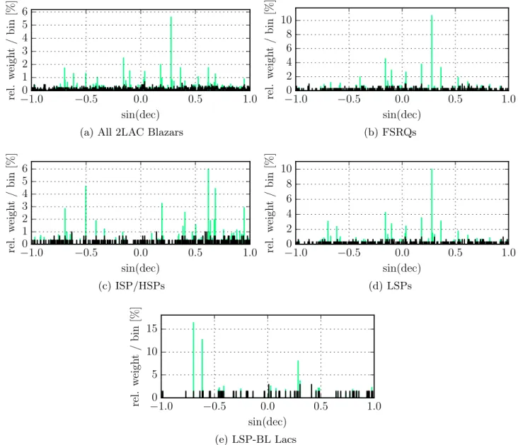
The distribution of the sources in the sky for the largest sample(all 2LAC blazars) and smallest sample (LSP-BL Lacs) is shown in Figure 1. A modest LAT-exposure deficit and lower sky coverage by optical surveys in the southern sky lead to a slight deficit of objects in the southern hemisphere (Ackermann et al.2011). The effect is most prominent for the

BL Lac-dominated samples. However, blazars without optical association are also included in the 2LAC catalog and partly make up for this asymmetry in the total sample. For simplicity, we assume a quasi-isotropic source distribution for all populations (excluding the source-free region around the galactic plane) for the calculation of quasi-diffuse fluxes. This assumption also seems reasonable given the weight distribution of sources (equal weighting) in Figures 9(a)–(e) and

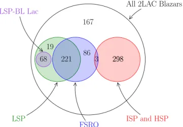
AppendixD. Figure2shows the overlap between the samples. The LSP-BL Lac, FSRQ, and ISP+HSP samples are nearly independent of one another, with a small overlap of 3 sources between the FSRQ and ISP+HSP samples. The largest overlap exists between the FSRQ and LSP samples, which share around 60% of their sources. The all-blazar sample contains 167 sources that are not shared with any subsample. These are

sources that are either unclassified or only classified as BL Lac objects with no corresponding synchrotron peak classification.

3. DATA SELECTION

IceCube is a neutrino telescope located at the geographic South Pole. It consists of about one km3_{of Antarctic ice that is}

instrumented with 5160 optical photosensors which are connected via cables (“strings”) with the data aqcuisition system at the surface. The photosensors detect Cherenkov light emitted by charged particles that are produced in the interactions of neutrinos with nuclei and electrons in the glacial ice. The geometry and sensitivity of the photosensors lead to an effective energy threshold of about 100 GeV for neutrinos. A more detailed description of the detector and the data acquisition can be found in Abbasi et al.(2009).

Two main signatures can be distinguished for the recorded events:“track-like” and “shower-like.” Only track-like events are of interest for the analysis here. They are the characteristic signature of muons produced in the charged-current interac-tions of muon neutrinos.59

Figure 1. Distribution of sources in the sky for the largest and smallest samples of blazars (in equatorial Mollweide projection)—(left) the largest sample, all 2LAC blazars(862 sources), and (right) the smallest sample, LSP-BL Lacs (68 sources). The excluded region of the catalog (∣ ∣ b 10) is highlighted in red.

Figure 2. Visualization of the source overlap between the different blazar populations.

59

We neglect track-like signals from nt+N +t Xm+X , i.e., muons as end products of a nt charged-current interaction chain. The tm decay happens with a branching fraction of only 17%(Olive2014), and the additional decay step lowers the outgoing muon energy, leading to even further suppression of the nt contribution in a sample of track-like events. For hard fluxes (spectral index 1–2) above PeV energies, where the ntinfluence becomes measurable due to nt regeneration (Bugaev et al. 2004), this treatment is conservative.

IceCube was constructed between 2006 and 2011 with a final configuration of 86 strings. We use data from the 59-string (IC-59), 79-string (IC-79), and 86-string (IC-86) configurations of the IceCube detector recorded between May 2009 and April 2012. In contrast to previous publications, we do not include data from the 40-string configuration here since the ice model description in the IC-40 Monte Carlo data sets is substantially different and the sensitivity gain would be marginal. The track event selection for the three years of data is similar to the one described in Aartsen et al. (2013b, 2014b). The angular

resolution of the majority of events in the track sample is better than 1° for events with reconstructed muon energies above 10 TeV (Aartsen et al. 2014b). The angular reconstruction

uncertainty is calculated following the prescription given in Neunhoffer (2006). We apply one additional minor selection

criterion for the estimated angular uncertainty of the recon-structed tracks (sest.5) for computational reasons. The removed events do not have any measurable effect on the sensitivity. Event numbers for the individual data sets are summarized in Table 1.

The data set is dominated by bundles of atmospheric muons produced in cosmic-ray air shower interactions for tracks coming from the southern hemisphere(q <90). Tracks from the northern hemisphere ( q 90) originate mostly from atmospheric neutrino interactions that produce muons. In order to reduce the overwhelming background of direct atmospheric muons to an acceptable level, it is necessary to impose a high-energy cut for events from the southern hemisphere. The cut raises the effective neutrino energy threshold to approximately 100 TeV (Aartsen et al. 2014b), reducing the sensitivity to

neutrino sources in this region by at least 1 order of magnitude for spectra softer than E-2_{. Only for harder spectra does the}

southern sky have a significant contribution to the overall sensitivity. The northern sky does not require such an energy cut, as upgoing tracks can only originate from neutrino interactions, which have a much lower incidence rate. However, at very high energies (again around 100 TeV), the Earth absorbs a substantial fraction of neutrinos, reducing the expected astrophysical signal as well. Charged-current nm

interactions can happen far outside the instrumented volume and still be detected, as high-energy muons may travel several kilometers through the glacial ice before entering the detector. This effect increases the effective detection area for certain arrival directions, mostly around the horizon.

The most sensitive region is therefore around the celestial equator, which does not require a high-energy cut, provides ample target material surrounding the detector, i.e., a large effective area, and does not suffer from absorption of neutrinos above 100 TeV. However, these zenith-dependent sensitivity changes are mostly important for the interpretation of the

results (see, e.g., Section5.3). The likelihood approach takes

these differences into account with the “acceptance” term in Equation(6), Section4.1, and a separation into several zenith-dependent analyses is not necessary. For more details on the properties of the data sets and the zenith-dependent sensitivity behavior, we refer the reader to Aartsen et al. (2013b) and

Aartsen et al.(2014b).

4. ANALYSIS

4.1. The Likelihood Function for Unbinned ML Stacking Analysis is performed via an extended unbinned maximum-likelihoodfit (Barlow 1990). The likelihood function consists

of two PDFs, one PDFB x( )for a background hypothesis and one PDF S x( ) for a signal hypothesis. Requiring the total number of observed events to be the sum of the signal and background events, the log-likelihood function can be written as ( ){ } · ( ) · ( ( ) ) ( )

å

where i indexes individual neutrino events. The likelihood function depends on two free parameters: the normalization factor ns and spectral index GSI of the total blazar signal. For

computational reasons we assume that each source of a given population shares the same spectral index. The background evaluation for each event depends on the reconstructed declination diand the reconstructed muon energy ei. The signal

part additionally depends on the reconstructed right ascension R.A.i, the angular error estimator si, and the power-law spectral

index GSI.

The background PDF is constructed from binning the recorded data in the reconstructed declination and energy. It is evaluated as ( ( )d e) · ( ( ) ) ( ) p d e = B sin , 1 f 2 sin , , 2 i i i i where p 1

2 arises from integration over the right ascension and f

is the normalized joint probability distribution of the events in declinationsin( )d and energyε.

The signal PDF that describes a given blazar population is a superposition of the individual PDFs for each source,

( ) · ( ) ( )

å

å

where wjis a weight determining the relative normalization of

the PDF Sjfor source j. This weight therefore accounts for the

relative contribution of source j to the combined signal. In general, different choices of wj are possible. The two choices

used in this work are discussed in Section4.2. Each term Sjin

Table 1

Total Number of Data Events in the Respective Data Sets of IC-59, IC-79, and IC-86 for Each Celestial Hemisphere

Data Set All Sky Northern Sky Southern Sky

IC-59 107011 42781 64230

IC-79 93720 48782 44938

IC-86 136245 61325 74920

Note.“Northern sky” means the zenith angle θ for the incoming particle directions is equal to or larger than 90°. “Southern sky” means q <90 .

Equation(3) is evaluated as ( ) · · [ ] · ( ) ( ) d s e ps d s e G = ⎛ Y G ⎝ ⎜⎜ ⎛_⎝⎜ ⎞ ⎠ ⎟ ⎞ ⎠ ⎟⎟ S g , R.A. , , ; 1 2 exp 1 2 , R.A. ; , 4 j i i i i i ij i i i j i SI 2 2 SI

where the spatial term is expressed as a 2D symmetric normal distribution and gjis the normalized PDF for the reconstructed

muon energy for source j. The term Yijis the angular separation

between event i and source j.

4.2. Weighting Schemes

The term wj in Equation (3) parametrizes the relative

contribution of source j to the combined signal. It corresponds to the expected number of events for source j and can be expressed as · ( ) · ( ) ( )

ò

where Aeff(qj,En) is the effective area for incoming muon neutrinos from a given source direction at a given energy,

( n)

h Ej denotes the normalized neutrino energy spectrum for

source j, and F0,j is its overall flux normalization. The

integration bounds En,min and En,max are set to 102 and

10 GeV9 _{, respectively, except for the differential analysis(see}

Section 4.3), in which they are defined for the given

energy band.

Under the assumption that all sources share the same spectral power-law shape, wjis further simplified via

[ ] · ( ) · ( ) [ · ] · [ ( )] ( )

ò

and splits into a“model” term wj,model—which is proportional

to the expected relative neutrino flux of source j—and an “acceptance” term, which is fixed by the position of the source and the global energy spectrum. The term wj,modelis not known,

and its choice defines the “weighting scheme” for the stacking analysis. The following two separate weighting schemes are used for the signal PDF in the likelihood analysis, leading to two different sets of tests.

4.2.1.γ-weighting

For this weighting scheme, wefirst have to assume that the γ-ray flux can be modeled to be quasi-steady between 2008 and 2010, the time period which forms the basis for the 2LAC catalog. This makes it possible to extrapolate the flux expectation of each source to other time periods, e.g., into the non-overlapping part of the data-taking period of the IceCube data for this analysis (2009–2012). Each model weight, i.e., the relative neutrinoflux expected to arrive from a given source, is then given by the source’s γ-ray energy flux observed by Fermi-LAT in the energy range between

>

E 100 MeV andE>100 GeV:

( )

ò

This is motivated by the fact that a similar amount of energy is channeled into the neutrino andγ-ray emission if pion decay from pp or pg interactions dominates the high-energy interaction. While the source environment is transparent to high-energy neutrinos, it might not be for γ-rays. The reprocessing of γ-rays due to gg interactions might then shift the energies of the photons to GeV and sub-GeV energies before they can leave the sources, which would make them detectable by the Fermi-LAT. This might even be expected in

g

p scenarios (Murase et al. 2015). Since a large fraction of

blazars are located at high redshiftsz1,60this reprocessing will also take place during the propagation of photons in extragalactic background light (EBL), shifting γ-ray energies below a few hundred GeV for such sources (Domínguez et al. 2013). This again potentially places them in the energy

range of the Fermi-LAT 2LAC catalog. Even in the case where synchrotron contributions (e.g., muon or pion synchrotron radiation) dominate pion decay in the MeV–GeV range, which has been considered for BL Lac objects in particular (Mücke et al.2003), one would expect the overall γ-ray emission to be

proportional to the neutrino emission. This is also the case in models where inverse Compton processes dominate the high-energyγ-ray emission (Murase et al.2014).

The preceding arguments in favor of aγ-weighting scheme assume that all sources show equal proportionality. On a source-by-source basis, however, the proportionality factor can vary, as already mentioned in Section1.

One contributing factor is the fact that Fermi probes different sections of the blazarγ-ray peak for each source relative to the peak position. For simplicity, we do not perform a spectral source-by-source fit in this paper, leaving this aspect for potential future work. This is also mostly an issue for the“all 2LAC blazar” sample, since the other subclassifications described in Section 2 depend on the peak position and this effect is largely mitigated. There are additional reasons for source-by-source fluctuations in the g n correlation due to EBL reprocessing. First, EBL absorption might not be sufficient for close-by sources, such that emerging high-energy γ-rays are not reprocessed into the energy range of the 2LAC catalog, which ends at 100 GeV. Second, EBL reprocessing differs between sources depending on the line-of-sight magn-etic fields, which deflect charged particle pairs produced in EBL cascades differently(Aharonian et al.1994). Third, strong

in-source gg reprocessing could lead to γ-rays at even lower energies than 100 MeV(Murase et al.2015), which would be

below the 2LAC energy range.

All results presented in Section5 based on theγ-weighting scheme assume that the potential source-to-sourcefluctuations in the g n correlation described here average out for large– source populations and can be neglected. More information on the distribution of weights according to declination can be found in Figures9(a)–(e) and AppendixD.

4.2.2. Equal Weighting

The γ-weighting scheme is optimal under the assumption that the neutrino flux follows the measured γ-energy flux exactly. Given the uncertainties discussed in Section4.2.1, we 60

also use another weighting scheme,

( ) =

wj,model 1, 8

which we expect to be more sensitive eventually if the actual –

g n correlation varies strongly from source to source. It

provides a complementary and model-independent test which is maximally agnostic to the degree of correlation between γ-ray and neutrino luminosities.

We do not assume a specific neutrino emission—equal emission in particular—in a given source when calculating the flux upper limits for the equal-weighting scheme. We only assume, to some approximation, that the differential source count distributions (SCDs) of γ-rays and neutrinos have comparable shapes. The differential SCD, dN/dS, describes how the energy-integratedflux S is distributed over all sources, and is a crucial property of any cosmological source population. Section 4.4 provides more information on the technical aspects of neutrino flux injection in the equal-weighting test. AppendixAthen discusses why the methodol-ogy is robust against variations in the actual shape of the dN/dS distribution for the neutrino flux in the IceCube energy range and why the final result is valid even if the neutrino SCD is different from the γ-ray SCD.

4.3. Statistical Tests

We perform statistical tests for each population of blazars. The log-likelihood difference λ defines our test statistic (TS), given by · ( ){ } · ( ){ } ( ) l = - = + = G = G L n L n n 2 log 0 2 log , , 9 s s s,max SI SI,max

where ns,max and GSI,maxare the number of signal events and the

signal spectral index that maximize the TS. We simulate an ensemble of background-only skymaps where the TS distribu-tion is compared with the TS value obtained from the data. The p-value is then defined as the fraction of skymaps in the background ensemble that has a larger TS value than the one observed. Ensembles of skymaps with different injected signal strengths are then used to calculate the resulting confidence interval. See Section4.4for details on the skymap simulations. In total we perform two distinct types of tests for which p-values are calculated. The first (“integral”) assumes a power-law spectrum for the blazar emission over the full energy range observable with IceCube(unless stated otherwise). The second (“differential”) assumes a neutrino signal that is confined to a small energy range(half a decade in energy), and has a power-law spectrum with a spectral index of−2 within this range. We perform the differential test for 14 energy ranges between 100 GeV and 1 EeV.

4.4. Simulations

We estimate the sensitivity of our searches in both weighting schemes using an ensemble of simulated skymaps containing both background and signal events.

We simulate the background by drawing events from the experimental data sample and then randomizing their right ascensions to remove any correlation with the blazar positions. This is the same method used in previous IceCube point source searches (Aartsen et al. 2013b, 2014b), and it mitigates

systematic uncertainties in the background description due to the data-driven event injection.

The injection for signals differs depending on the weighting scheme. For the γ-weighting scheme, we inject signal events with the relativeflux contribution of each source determined by the weight factors wj,model that are used in the PDF. In the

equal-weighting scheme, following the same approach would lead to a simulated signal of n equally bright sources, which is not realistic for a population distributed widely in redshift and luminosity. Therefore, we inject events using a relative neutrino flux contribution that follows a realistic SCD. Since the neutrino dN/dS distribution of blazars is unknown, we have chosen to use the blazar γ-ray SCD published in Abdo et al. (2010c) as a template.61Here we assume that for the population under investigation, the relative contributions to the total neutrino flux are distributed in a similar fashion to the distribution of the relative contributions to the totalγ-ray flux. However, there are no assumptions about the correlation of the neutrino andγ-ray flux for individual sources.

We choose theγ-ray SCD as the primary template for the shape of the neutrino SCD for two reasons. Thefirst is that we select the populations based on their γ-ray emission to start with. The second is that the form of the high-energyγ-ray SCD is quite general and has also been observed with AGNs detected in the radio (Hopkins et al. 2003) and X-ray

(Georgakakis et al.2008) bands. It starts with quasi-Euclidean

behavior (S5 2·dN dS»const._{) at high fluxes and then} changes to a harder power-law index toward smaller flux values, which ensures that the total flux from the population remainsfinite.

The skymap simulations are performed for many possible SCD realizations by sampling from the dN/dS distribution. This is necessary since the number of signal events expected in IceCube for a given neutrino flux varies greatly over the two hemispheres(see Section3). Thus, it matters how the neutrino

flux is distributed over the individual sources for the value of the resulting confidence interval. The shape of the SCD and the flux sampling range have an additional impact. See Appendix A for further details in the context of confidence interval construction.

5. RESULTS 5.1. Observed p-Values

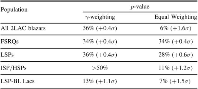
Table2 summarizes the p-values for the“integral” test (see Section4.3). Nine out of the ten tests show overfluctuations but

no significant excess. We find the strongest overfluctuation, a 6% p-value, using the equal-weighting scheme for all 2LAC blazars. We omit a trial-factor correction because the popula-tions have a large overlap and the result is not significant.

Figure 3 shows the p-values from the corresponding “differential” test. The largest excess is visible in the 5–10 TeV energy band with a pre-trial p-value of 4·10-3_.

This outcome is totally compatible with a fluctuation of the background, since the effect of multiple trials has to be taken into account, reducing the significance of the observation substantially. Accurate calculation of the trial-corrected p-value is again difficult, as neither the five blazar samples nor the 14 61

This blazar SCD strictly stems from the 1FGL catalog(Abdo et al.2010b), but any SCD based on a newer catalog is not expected to change significantly since a large fraction of the totalγ-ray flux is already resolved in the 1FGL.

tested energy ranges per sample are independent. We again omit it for simplicity.

Comparing the differential p-value plot of all 2LAC blazars with that of the other populations (see Figures 10(a)–(e) in

AppendixD), one finds that the overfluctuation is caused by the

LSP-BL Lac, FSRQ, and ISP/HSP populations, which are nearly independent of one another and show a small excess in the 5 TeV–20 TeV region. In the γ-weighting scheme, the ISP/ HSP p-value distribution is nearly flat, which leads to an overfluctuation in the all 2LAC blazar sample that is weaker than that in the equal-weighting scenario.

5.2. Flux Upper Limits

Since no statistically significant neutrino emission from the analyzed source populations was found, we calculate the flux upper limits using various assumptions about their energy spectrum. We use the CLsupper limit construction(Read2000).

It is more conservative than a standard Neyman construction, e.g., as used in Aartsen et al.(2014b), but allows for a proper

evaluation of underfluctuations of the background, which is used for the construction of differentialflux upper limits.

We give all further results in intensity units and calculate the quasi-diffuse flux62for each population. Theflux upper limits in the equal-weighting scheme are calculated using multiple

samplings from an assumed neutrino SCD for the blazars, as already outlined in Section4.4. Please refer to AppendixAfor further details about the dependence of theflux upper limit on the choice of SCD and a discussion of the robustness of the equal-weighting results. In general, the equal-weighting upper limit results do not correspond to a singleflux value but span a range offlux values.

For each upper limit63we determine the valid energy range according to the procedure in AppendixB. This energy range specifies where IceCube has exclusion power for a particular model, and is also used for visualization purposes in allfigures. Systematic effects influencing the upper limits are dominated by uncertainties on the absorption and scattering properties of the Antarctic ice and the detection efficiency of the optical modules. Following Aartsen et al.(2014b), the total systematic

uncertainty on the upper limits is estimated to be 21%. Since we are dealing with upper limits only, we conservatively include the uncertainty additively in allfigures and tables.

5.3. Generic Upper Limits

Table3 showsflux upper limits assuming a generic power-law spectrum for the tested blazar populations, calculated for the three different spectral indices:−1.5, −2.0, and −2.7.

The distribution of theγ-ray energy flux among the sources in each population governs theflux upper limit in the γ-weighting scheme. It is mostly driven by the declination of the strongest sources in the population, due to the strong declination dependence of IceCube’s effective area. For FSRQs, the two sources with the largestγ-weights (3C 454.3 atdecl.2000 =16 andPKS1510-08 atdecl.2000 = - 9 ) carry around 15% of the totalγ-weight of all FSRQs. Their positions close to the equator place them in the most sensitive region for the IceCube detector, and the γ-weighting upper limits for FSRQs are more than a factor of 2 lower than the corresponding equal-weighting limits. For the LSP-BL Lacs, the two strongest sources (PKS 0426-380 at decl.2000 = - 38 and PKS 0537-441 at

= - 

decl.2000 44) carry nearly 30% of the total γ-weight but are located in the southern sky, where IceCube is not very sensitive. Theγ-weighting upper limit is therefore comparable to the equal-weighting upper limit. The reader is referred to AppendixDfor more information on the weight distribution.

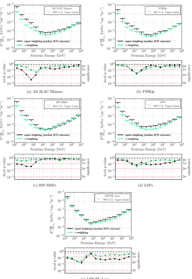
Figure4shows the differential upper limit in comparison to the median sensitivity for all 2LAC blazars using the equal-weighting scheme. This population showed the largest over-fluctuation. We plot here the upper limit derived from the median SCD sampling outcome, since in general the equal-weighting upper limit depends on the neutrinoflux realization of the SCD (see Appendix A). As expected, the differential

limit is slightly higher, by a factor of about 2, than the median outcome in the energy range between 5 and 10 TeV, where the largest excess is observed. This is the average behavior for a softflux with a spectral index of about −3.064if one assumes a simple power-lawfit to explain the data. While such a physical interpretation cannot be made yet, it will be interesting to observe this excess with future IceCube data. For information on the differential upper limits from the other samples, the reader is referred to AppendixD.

Table 2

p-Values and the Corresponding Significance in Units of Standard Normal Deviations in the Power-Law Test

Population p-value

γ-weighting Equal Weighting

All 2LAC blazars 36% (+0.4s) 6% (+1.6s)

FSRQs 34% (+0.4s) 34% (+0.4s)

LSPs 36% (+0.4s) 28% (+0.6s)

ISP/HSPs >50% 11% (+1.2s)

LSP-BL Lacs 13% (+1.1s) 7% (+1.5s)

Note.The table shows the results for both weighting schemes. The values do not include a trial-factor correction.

Figure 3. Local p-values for the sample containing all 2LAC blazars using the equal-weighting scheme (black) and γ-weighting scheme (green) in the differential test.

62

Theflux divided by the solid angle of the sky above 10° galactic latitude, i.e.,0.83´4 . See Sectionp 2for a justification.

63

With the exception of the differential upper limit. 64

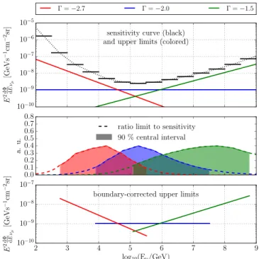
This can be read off in Figure8. The ratio function indicates in which energy range a givenflux function appears first, on average.

5.4. The Maximal Contribution to the Diffuse Astrophysical Flux

Astrophysical neutrinoflux is observed between 10 TeV and 2 PeV(Aartsen et al.2015b). Its spectrum has been found to be

compatible with a single power law and a spectral index of −2.5 over most of this energy range. Accordingly, we use a power law with the same spectral index and a minimum neutrino energy of 10 TeV for the signal injected into the simulated skymaps when calculating the upper limit for a direct comparison. Figure5 shows theflux upper limit for an E-2.5

power-law spectrum starting at 10 TeV for both weighting schemes in comparison to the most recent global fit of the astrophysical diffuse neutrino flux, assuming an equal composition offlavors arriving on Earth.

The equal-weighting upper limit results in a maximal 19%– 27% contribution of the total 2LAC blazar sample to the observed best-fit value of the astrophysical neutrino flux, including systematic uncertainties. This limit is independent of the detailed correlation between the γ-ray and neutrino flux from these sources. The only assumption is that the respective neutrino andγ-ray SCDs have similar shapes (see Section5.2

for details on the signal injection). We use the Fermi-LAT blazar SCD published in Abdo et al.(2010c) as a template for

sampling. However, wefind that even if the shape of the SCD differs from the shape of this template, the upper limit still holds and is robust. In Appendix Awe discuss the effect of different SCD shapes and how combination with existing point source constraints(Aartsen et al.2015c) leads to a nearly

SCD-independent result, since a point source analysis and a stacking search with equal weights effectively trace opposite parts of the available parameter space for the dN/dS distribution.

If we assume proportionality between theγ-ray and neutrino luminosities of the sources, theγ-weighting limit constrains the maximal flux contribution of all 2LAC blazars to 7% of the observed neutrinoflux in the full 10 TeV to 2 PeV range. Since the blazars resolved in the 2LAC account for 70% of the total γ-ray emission from all GeV blazars (Ajello et al.2015), this

further implies that at most 10% of the astrophysical neutrino flux stems from all GeV blazars extrapolated to the whole Table 3

90% C.L. Upper Limits on the Diffuse(nm+nm) Flux from the Different Blazar

Populations Tested Spectrum:F0· (E GeV)-1.5

Blazar Class F090%[GeV-1cm-2s-1sr-1]

γ-weighting Equal Weighting

All 2LAC Blazars 1.6´10-12 _{4.6 3.8 5.3( – ) ´10}-12

FSRQs 0.8´10-12 _{2.1 1.0 3.1( – ) ´10}-12

LSPs 1.0´10-12 _{1.9 1.2 2.6( – ) ´10}-12

ISPs/HSPs 1.8´10-12 _{2.6 2.0 3.2( – ) ´10}-12 LSP-BL Lacs 1.1´10-12 _{1.4 0.5 2.3( – ) ´10}-12

Spectrum:F0· (E GeV)-2.0

Blazar Class F090%[GeV-1cm-2s-1sr-1]

γ-weighting Equal Weighting

All 2LAC Blazars 1.5´10-9 _{4.7 3.9 5.4( – ) ´10}-9

FSRQs 0.9´10-9 _{1.7 0.8 2.6( – ) ´10}-9

LSPs 0.9´10-9 _{2.2 1.4 3.0( – ) ´10}-9

ISPs/HSPs 1.3´10-9 _{2.5 1.9 3.1( – ) ´10}-9

LSP-BL Lacs 1.2´10-9 _{1.5 0.5 2.4( – ) ´10}-9 Spectrum:F0· (E GeV)-2.7

Blazar Class F090%[GeV-1cm-2s-1sr-1]

γ-weighting Equal Weighting

All 2LAC Blazars 2.5´10-6 _{8.3 7.0 9.7( – ) ´10}-6

FSRQs 1.7´10-6 _{3.3 1.6 5.1( – ) ´10}-6

LSPs 1.6´10-6 _{3.8 2.4 5.2( – ) ´10}-6

ISPs/HSPs _1.6´₁₀-6 _{4.6 3.5 5.6( – ) ´10}-6

LSP-BL Lacs 2.2´10-6 _{2.8 1.0 4.6( – ) ´10}-6 Note.The table contains results for power-law spectra with spectral indices of −1.5, −2.0, and −2.7. The equal-weighting column shows the median flux upper limit and the 90% central interval of different sample realizations of the Fermi-LAT source count contribution (in parentheses). All values include systematic uncertainties.

Figure 4. Differential 90% C.L. upper limit on the (nm+nm) flux using equal

weighting for all 2LAC blazars. The1 ands 2 null expectation is showns in green and yellow, respectively. The upper limit and expected regions correspond to the median SCD sampling outcome.

Figure 5. 90% C.L. flux upper limits for all 2LAC blazars in comparison to the observed astrophysical diffuse neutrino flux. The latest combined diffuse neutrinoflux results from Aartsen et al. (2015b) are plotted as the best-fit power law with a spectral index of−2.5 and as a differential flux unfolding using 68% central and 90% U.L. confidence intervals. The flux upper limit is shown using both weighting schemes for a power law with a spectral index of−2.5 (blue). Percentages denote the fraction of the upper limit compared to the astrophysical best-fit value. The equal-weighting upper limit for a flux with a harder spectral index of−2.2 is shown in green.

universe, again in the full 10 TeV to 2 PeV range and assuming the γ-weighting is an appropriate weighting assumption. Table 4 summarizes the maximal contributions for all populations, including the γ-weighting result scaled to the respective total population of sources in the observable universe.

It is interesting to compare these numbers directly to the γ-ray sector. Ajello et al. (2015) show that GeV blazars

(100 MeV–100 GeV) contribute approximately 50% to the extragalactic gamma-ray background. The resolved 1FGL (Abdo et al.2010b) blazar component in particular contributes

around 35%. This estimate should be rather similar for the 2LAC blazars studied here, which are defined based on the more recent 2FGL catalog(Nolan et al.2012) (see AppendixC

for a discussion). The 2LAC blazar contribution to the astrophysical neutrino flux is therefore at least a factor of 0.75 smaller than the corresponding extragalactic contribution in theγ-regime. The difference of this contribution between the two sectors becomes substantial (7% maximally allowed contribution for neutrinos versus 35% for γ-rays) if one assumes aγ/ν-correlation.

Figure 5 also shows the equal-weighting constraint for a harder neutrino spectrum with a spectral index of −2.2. This harder spectral index is about 3 standard deviations away from the best-fit value derived in Aartsen et al. (2015b) and can be

used as an extremal case given the current observations. Comparison of this upper limit with the hard end of the “butterfly” shows that even in this case less than half of the bulk emission can originate in the 2LAC blazars with minimal assumptions about the relative neutrino emission strengths. Due to the low-count status of the data, we omit multi power-law spectrum tests at this point. However, one can estimate the constraints for more complicated models using Figure 8 in Appendix B, which shows the energy range for a given spectrum that contributes the dominant fraction to the sensitivity. The sensitivity for a possible two-component model that has, for example, a soft component at TeV energies and a hard component in the PeV range would be dominated by the soft regime, as the“ratio function” (see AppendixB, Figure8)

by the hard component above a PeV is negligible. In such a scenario, we expect the constraint to be rather similar to our result from the simple power-law test with a spectral index of −2.5.

5.5. Upper Limits on Models for Diffuse Neutrino Emission For experimental constraints on existing theoretical calcula-tions, we only considered models for diffuse emission from blazar populations, not predictions for specific objects. These include the calculations by Mannheim (1995), Halzen & Zas

(1997), and Protheroe (1997) for generic blazars; the

calcula-tions by Becker et al. (2005) and Murase et al. (2014) for

FSRQs; and the calculations by Mücke et al.(2003), Tavecchio

et al. (2014), Tavecchio & Ghisellini (2015), and Padovani

et al.(2015) for BL Lacs.

The upper limits in this section are calculated using the γ-weighting scheme and therefore assume a correlation between the neutrino flux and the measured γ-ray energy flux. This allows us to account for the fraction of the neutrino emission that arises from blazars not detected inγ-rays. The fraction of γ-ray emission from resolved 2LAC blazars in general (including BL Lacs) and from FSRQs in particular is about 70%(Ajello et al.2015,2012). Therefore, the flux upper limits

for the entire population are a factor of1 0.7 »1.43 weaker than those derived for the quasi-diffuse flux of the 2LAC blazars. See AppendixCfor more details on this factor.

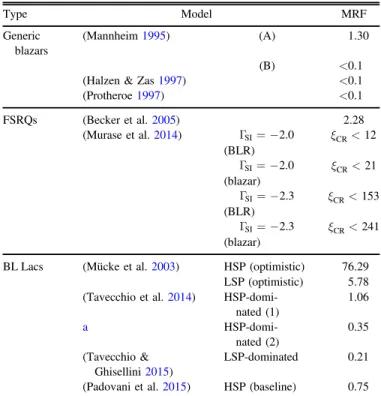
Table 5 summarizes the model rejection factors (Hill & Rawlins 2003)65 for all considered models. Many of these models can be constrained by this analysis. Figures 6(a)–(d)

Table 4

Maximal Contributions to the Best-fit Diffuse Flux from Aartsen et al. (2015b) Assuming the Equipartition of Neutrino Flavors

Population Weighting Scheme

Equal γ γ (Extrapol.)

all 2LAC blazars 19%–27% 7% 10%

FSRQs 5% 17%– 5% 7%

LSPs 6% 15%– 5% 7%

ISP/HSPs 9% 15%– 5% 7%

LSP-BL Lacs 3% 13%– 6% 9%

Note.The equal-weighting case shows this maximal contribution for the 90% central outcomes of potential dn/ds realizations. The last column shows the maximal contribution of the integrated emission from the total parent population in the observable universe exploiting the γ-ray completeness of the 2LAC blazars(see AppendixC).

Table 5

Summary of Constraints and Model Rejection Factors for the Diffuse Neutrino Flux Predictions from Blazar Populations

Type Model MRF

Generic blazars

(Mannheim1995) (A) 1.30

(B) <0.1

(Halzen & Zas1997) <0.1

(Protheroe1997) <0.1 FSRQs (Becker et al.2005) 2.28 (Murase et al.2014) G = -2.0SI (BLR) x_CR< 12 G = -2.0SI (blazar) xCR< 21 G = -2.3SI (BLR) x_CR< 153 G = -2.3SI (blazar) xCR< 241 BL Lacs (Mücke et al.2003) HSP(optimistic) 76.29

LSP(optimistic) 5.78 (Tavecchio et al.2014)

HSP-domi-nated(1) 1.06 a HSP-domi-nated(2) 0.35 (Tavecchio & Ghisellini2015) LSP-dominated 0.21

(Padovani et al.2015) HSP(baseline) 0.75 Notes. The values include a correction factor for unresolved sources (see AppendixC) and systematic uncertainties. For models involving a range of flux predictions, we calculate the MRF with respect to the lower flux of the optimistic templates(Mücke et al.2003) or to constraints on the baryon-to-photon luminosity ratios xCR(Murase et al.2014).

a

Predictions from Tavecchio et al.(2014) and Tavecchio & Ghisellini (2015) enhanced by a factor of 3 in correspondence with the authors.

65

visualize the flux upper limits in comparison to the neutrino flux predictions.

In early models (before the year 2000) the neutrino flux per source is calculated to be directly proportional to theγ-ray flux in the energy range Eg >100 MeV (Mannheim 1995)

(A), Eg >1 MeV (Mannheim 1995) (B), 20 MeV<Eg <

30 GeV (Halzen & Zas 1997), and Eg >100 MeV

(Protheroe 1997). The γ-weighting scheme is therefore almost

implicit in all these calculations, although the energy ranges vary slightly from the100 MeV 100 GeV energy range used for the– γ-weighting.

Among the newer models, only Padovani et al.’s (2015) uses

a direct proportionality between the neutrino andγ-ray flux (for >

g

E 10 GeV), where the proportionality factor encodes a

possible leptonic contribution. In all other publications a direct correlation to γ-rays is not used for the neutrino flux calculation. Since all these models assume that p/γ-interactions dominate the neutrino production, the resulting neutrinofluxes are calculated via the luminosity in the target photonfields. In Becker et al. (2005) the neutrino flux is proportional to the

target radio flux, which in turn is connected to the disk luminosity via the model from Falcke & Biermann(1995). In

Mücke et al.(2003) the neutrino flux is directly proportional to

the radiation of the synchrotron peak. In Murase et al.(2014)

the neutrinoflux is connected to the X-ray luminosity, which in turn is proportional to the luminosity in various target photon fields. In Tavecchio et al. (2014) the neutrino luminosity is

calculated using target photon fields from the inner jet “spine layer.” However, a correlation to the γ-ray flux in these latter

models may still exist, even in the case where leptonicγ-ray contributions dominate. This is mentioned in Murase et al. (2014), who explicitly predict the strongest γ-ray emitters to

also be the strongest neutrino emitters, even though the model contains leptonically produced γ-ray emission. It should be noted that an independent IceCube analysis studying the all-flavor diffuse neutrino flux at PeV energies and beyond (Aartsen et al. 2016a) recently also put strong constraints on

some of theflux predictions discussed in this section.

6. SUMMARY AND OUTLOOK

In this paper, we have analyzed all 862 Fermi-LAT 2LAC blazars and 4 spectrally selected subpopulations via an unbinned likelihood stacking approach for a cumulative neutrino excess from the given blazar directions. The study uses 3 years of IceCube data(2009–2012), which amount to a total of around 340000 muon-track events.

Each of the 5 populations was analyzed with two weighting schemes which encode assumptions about the relative neutrino flux from each source in a given population. The first weighting scheme uses the energy flux observed in γ-rays as weights, whereas the second scheme gives each source the same weight. This resulted in a total of 10 statistical tests, which were in turn analyzed in two different ways. Thefirst is an “integral” test, in which a power-lawflux with a variable spectral index is fitted over the full energy range that IceCube is sensitive to. The second is a differential analysis, in which 14 energy segments between 102 _{and 10 GeV}9 _{, each spanning half a decade in}

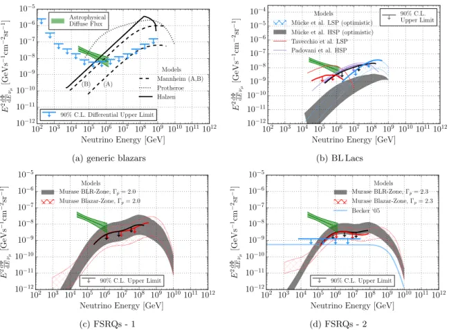
Figure 6. 90% C.L. upper limits on the (nm+nm) flux for models of the neutrino emission from (a) generic blazars (Mannheim1995; Halzen & Zas1997; Protheroe1997), (b) BL Lacs (Mücke et al.2003; Padovani et al.2015; Tavecchio & Ghisellini2015), and (c)+(d) FSRQs (Becker et al.2005; Murase et al.2014). The upper limits include a correction factor that takes into account theflux from unresolved sources (see AppendixC) and systematic uncertainties. The astrophysical diffuse neutrinoflux measurement (Aartsen et al.2015b) is shown in green for comparison.

energy, are fit independently with a constant spectral index of −2.

Nine of the ten integral tests show overfluctuations, but none of them are significant. The largest overfluctuation, a 6% p-value, is observed for all 862 2LAC blazars combined using the model-independent equal-weighting scheme. The differential test for all 2LAC blazars using equal source weighting reveals that the excess appears in the 5–10 TeV region with a local p-value of2.6 . No correction for testing multiple hypotheses iss applied, since even without a trial correction this excess cannot be considered significant.

Given the null results, we then calculated the flux upper limits. The two most important results of this paper are as follows:

1. We calculated a flux upper limit for a power-law spectrum starting at 10 TeV with a spectral index of −2.5 for all 2LAC blazars. We compared this upper limit to the diffuse astrophysical neutrino flux observed by IceCube (Aartsen et al. 2015b). We found that the

maximal contribution from all 2LAC blazars in the energy range between 10 TeV and 2 PeV is 27%,

including systematic effects and with minimal assump-tions about the neutrino/γ-ray correlation in each source. Changing the spectral index of the testedflux to −2.2, a value allowed at about 3 standard deviations given the current globalfit result (Aartsen et al. 2015b), weakens

this constraint by about a factor of two. If we assume for each source a similar proportionality between the γ-ray luminosity in the 2LAC energy range and the neutrino luminosity, we can extend the constraint to the parent population of all GeV blazars in the observable universe. The corresponding maximal contribution is then around 10% from all GeV blazars, or 5%–10% from the other blazar subpopulations. In each case, we use the same power-law assumption as before in order to compare it to the observed flux. For FSRQs our analysis allows for a 7% contribution to the diffuseflux, which is in general agreement with a result obtained by Wang & Li(2015),

who independently estimated that FSRQs do not contribute more than 10% to the diffuse flux using our earlier small-sample stacking result for 33 FSRQs (Aartsen et al.2014b).

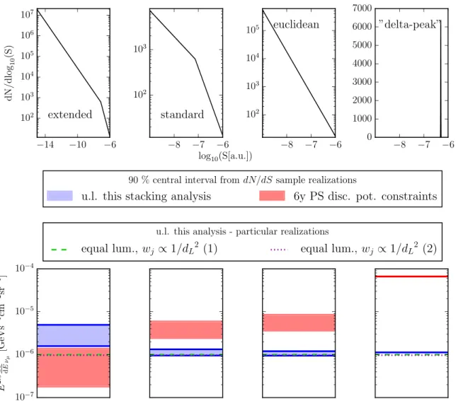
Figure 7. Comparison of equal-weighting upper limits for different SCDs which are used to sample relative source injection weights, shown for the population of all 2LAC blazars. The upper row shows the SCDs and the lower row the respective constraints for anE-2.5_{flux starting at 10 TeV. The source flux S on the x-axis is} shown in arbitrary units—since only the relative neutrino flux counts—but orients itself by the integrated γ-ray flux from Abdo et al. (2010c). The light blue band marks the 90% central interval of upper limit outcomes for random samplings of the given SCD, and the light red band marks the constraints from the 6-year PS search for similar random samplings. Two specific realizations modeling equal intrinsic luminosity and taking into account the luminosity distance and randomly drawn redshifts for missing-redshift BL Lacs are shown in green and magenta.

2. We calculated upper limits using theγ-weighting scheme for 15 models of the diffuse neutrino emission from blazar populations found in the literature. For most of these models, the upper limit constrains the model prediction—by more than an order of magnitude for some of them. The implicit assumption in all these upper limits is a proportionality between the source-by-source γ-ray luminosity in the 2LAC energy range and its corresponding neutrino luminosity. All models published before the year 2000 and the model by Padovani et al. (2015) implicitly contain this assumption, although some

of their energy ranges differ from the exact energy range in the 2LAC catalog. Even for the other models the proportionality assumption may still hold, as indicated by Murase et al. (2014).

Kadler et al.(2016) recently claimed a 5% probability for a

PeV IceCube event to have originated close to blazar PKS B1424-418 during a high-fluence state. While 5% is not yet statistical evidence, our results do not contradict such single PeV-event associations, especially since a dominant fraction of the sensitivity of our analysis comes from the sub-PeV energy range. The same authors also show that the measured all-sky PeV neutrinoflux cannot be compatible with an origin in a pure FSRQ population that has a peaked spectrum around PeV energies, as it would overpredict the number of observed events. Instead, one has to invoke additional assumptions—for example, a certain contribution from BL Lacs, leptonic contributions to the SED, or a spectral broadening of the arriving neutrino flux down to TeV energies due to Doppler shifts from the jets and the intrinsic redshift distribution of the blazars. Our results suggest that the last assumption, a spectrum broadening down to TeV energies, only works if the resulting power-law spectral index is harder than around −2.2, as the flux is otherwise in tension with our γ-weighting upper limit. A hard PeV spectrum is interestingly also seen by a recent IceCube analysis (Aartsen et al. 2016b) that probes the PeV

range with muon neutrinos. Regardless of these speculations, the existing sub-PeV data require an explanation beyond the 2LAC sample from a yet unidentified galactic or extragalactic source class.

Our results do not provide a solution to explain the bulk emission of astrophysical diffuse neutrinos, but they provide robust constraints that might help to construct the global picture. Recently, Murase et al. (2015) argued that current

observations favor sources that are opaque to γ-rays. This would, for example, be expected in the cores of AGNs. Our findings on the 2LAC blazars mostly provide a basis for probing the emission from relativistically beamed AGN jets and are in line with these expectations. We also do not constrain neutrinos from blazar classes that are not part of the 2LAC catalog—for example, extreme HSP objects. These sources may emit up to 30% of the diffuse flux (Padovani et al.2016), and studies in this direction with other catalogs are

in progress.

While the slight excess in the 5–10 TeV region is not yet significant, further observations by IceCube may clarify if what we see is an emerging soft signal or just a statisticalfluctuation. We acknowledge support from the following agencies: the U.S. National Science Foundation–Office of Polar Programs, the U.S. National Science Foundation–Physics Division, the University of Wisconsin Alumni Research Foundation, the

Grid Laboratory of Wisconsin’s grid infrastructure at the University of Wisconsin–Madison, and the Open Science Grid’s grid infrastructure; the U.S. Department of Energy’s National Energy Research Scientific Computing Center and the Louisiana Optical Network Initiative’s grid computing resources; the Natural Sciences and Engineering Research Council of Canada, WestGrid, and Compute/Calcul Canada; the Swedish Research Council, the Swedish Polar Research Secretariat, the Swedish National Infrastructure for Computing, and the Knut and Alice Wallenberg Foundation, Sweden; the German Ministry for Education and Research, Deutsche Forschungsgemeinschaft, the Helmholtz Alliance for Astro-particle Physics, and the Research Department of Plasmas with Complex Interactions (Bochum), Germany; the Fund for Scientific Research, FWO Odysseus program, Flanders Insti-tute (to encourage scientific and technological research in industry) and the Belgian Federal Science Policy Office; the University of Oxford, United Kingdom; the Marsden Fund, New Zealand; the Australian Research Council; Japan Society for Promotion of Science; the Swiss National Science Foundation, Switzerland; the National Research Foundation of Korea (NRF); and Villum Fonden, Danish National Research Foundation, Denmark.

APPENDIX A

DEPENDENCE OF FLUX UPPER LIMITS ON THE SCD SAMPLING

The equal-weighting limits use source count distributions to model the neutrino injection. The SCD serves as a PDF template from which relative neutrino injection weights are drawn. Depending on the shape of the SCD and the range of flux values in which the SCD is being sampled, the resulting central neutrino upper limit value shifts, and the range of Figure 8. Determination of the energy range that contributes 90% to the total sensitivity of IceCube for the neutrino flux of a given spectrum. The construction is shown for the total 2LAC blazar population using theγ-energy flux weighting scheme for three power-law spectra with spectral indices of −1.5, −2.0, and −2.7.