Counterfactual Policy Introspection using
Structural Causal Models
by
Michael Karl Oberst
B.A., Harvard University (2012)
Submitted to the Department of Electrical Engineering and Computer
Science
in partial fulfillment of the requirements for the degree of
Master of Science in Electrical Engineering and Computer Science
at the
MASSACHUSETTS INSTITUTE OF TECHNOLOGY
September 2019
c
○ Massachusetts Institute of Technology 2019. All rights reserved.
Author . . . .
Department of Electrical Engineering and Computer Science
August 30, 2019
Certified by . . . .
David Sontag
Associate Professor of Electrical Engineering and Computer Science
Thesis Supervisor
Accepted by . . . .
Leslie A. Kolodziejski
Professor of Electrical Engineering and Computer Science
Chair, Department Committee on Graduate Students
Counterfactual Policy Introspection using Structural Causal
Models
by
Michael Karl Oberst
Submitted to the Department of Electrical Engineering and Computer Science on August 30, 2019, in partial fulfillment of the
requirements for the degree of
Master of Science in Electrical Engineering and Computer Science
Abstract
Inspired by a growing interest in applying reinforcement learning (RL) to healthcare, we introduce a procedure for performing qualitative introspection and ‘debugging’ of models and policies. In particular, we make use of counterfactual trajectories, which describe the implicit belief (of a model) of ‘what would have happened’ if a policy had been applied. These serve to decompose model-based estimates of reward into specific claims about specific trajectories, a useful tool for ‘debugging’ of models and policies, especially when side information is available for domain experts to review alongside the counterfactual claims. More specifically, we give a general procedure (using structural causal models) to generate counterfactuals based on an existing model of the environment, including common models used in model-based RL. We apply our procedure to a pair of synthetic applications to build intuition, and con-clude with an application on real healthcare data, introspecting a policy for sepsis management learned in the recently published work of Komorowski et al. (2018).
Thesis Supervisor: David Sontag
Thesis Errata Sheet
Author _________________________________________________ Primary Dept. ___________________________________________ Degree ___________________ Graduation date____________ Thesis title _______________________________________________________________________________ _______________________________________________________________________________ _______________________________________________________________________________ Brief description of errata sheet _______________________________________________________________________________ _______________________________________________________________________________ _______________________________________________________________________________ _______________________________________________________________________________ _______________________________________________________________________________ Number of pages ____ (11
maximum, including this page) � Author: I request that the attached errata sheet be added to my thesis. I have attached two copies prepared as prescribed by the current Specifications for Thesis Preparation. Signature of author _____________________________________________ Date ___________ � Thesis Supervisor or Dept. Chair: I approve the attached errata sheet and recommend its addition to the students thesis. Signature _____________________________________________________ Date ___________ Name _________________________________________ Thesis supervisor Dept. Chair
� Vice Chancellor or his/her designee:
I approve the attached errata sheet and direct the Institute Archives to insert it into all copies of the students thesis held by the MIT Libraries, both print and electronic.
Signature _____________________________________________________ Date ___________ Name ________________________________________________________
Michael Karl Oberst EECS
MS 2019
Counterfactual Policy Introspection Using Structural Causal Models
I have corrected errors in the computational results presented in Chapter 7 of the thesis, which necessitated rewriting of the commentary and replacement of several figures 11 David Sontag 4 Ian A. Waitz 7/31/2020 July 1, 2020
Page 79, 2nd paragraph:
we find that there is only a single patient who would the we find there are a very small number of patients who the
Page 83, Table 7.1: Replace second/third row of table WIS (Validation): 53.82, 76.86, (-62.42, 99.29)
Model-based: 90.27, 90.30, (87.15, 93.30) WIS (Validation): 53.00, 76.64, (-73.00, 99.91) Model-based: 90.22, 90.20, (87.85, 92.70)
Page 83, Table 7.2: Replace second row of table WIS: 53.73, -99.99, 79.35, 100.00, 100.00, 100.00 WIS: 60.26, -28.42, 47.72, 69.42, 83.50, 96.59
Page 84, 2nd paragraph:
we find that only a single patient has we find that very few patients have
Page 84, Figure 7–2: Replace numbers 0%, 4%, 16% 0% 10% 70%
4%, 3%, 14%, 0%, 4%, 76%
Page 84, Figure 7–2 Caption:
only one patient. . . However, 14% of patients very few patients. . . However, 7% of patients
Page 85, end of first paragraph: under the estimated
under all their estimated
Page 85–87: Replace the text starting from This patient has two processes. . . until just before the start of the final paragraph on page 87 that begins with “In conclusion, if we are to fully trust”.
• Cause of admission: This patient was admitted after collapsing, with initial suspicion that this was due to either a respiratory or cardiac failure, and was taken immediately to the cath lab where cardiac causes were ruled out. Chest imaging showed a large amount of fluid around the right lung, and a large
mass in the lower right lobe. This was discovered to be State IIIA lung cancer, suggesting the possible etiology of the patients’ presentation to be cardiovascular collapse and a post-obstructive pneumonia secondary to compression from the mass.
• Treatment before and during ICU: Cardiovascular compromise and inflamma-tion from pneumonia contributed to the build up of a large amount of fluid in the pleural space. Thus, clinicians elected to place a chest tube, which sub-sequently drained >1L of serous fluid. The patient’s clinical status responded rapidly, suggesting the external compression from the fluid was a major con-tributor to his ICU course. Antibiotics and vasopressors in this setting act as temporizing measures until the definitive intervention of chest tube placement could be performed.
• Cause of death: Despite the placement of a chest tube, the underlying prob-lem of a large lung mass leading to cardiovascular compromise remained unad-dressed. Given the morbidity of the necessary chemotherapy, it was decided by the providers, the patient and the family that further aggressive intervention would not have been in the patient’s interests.
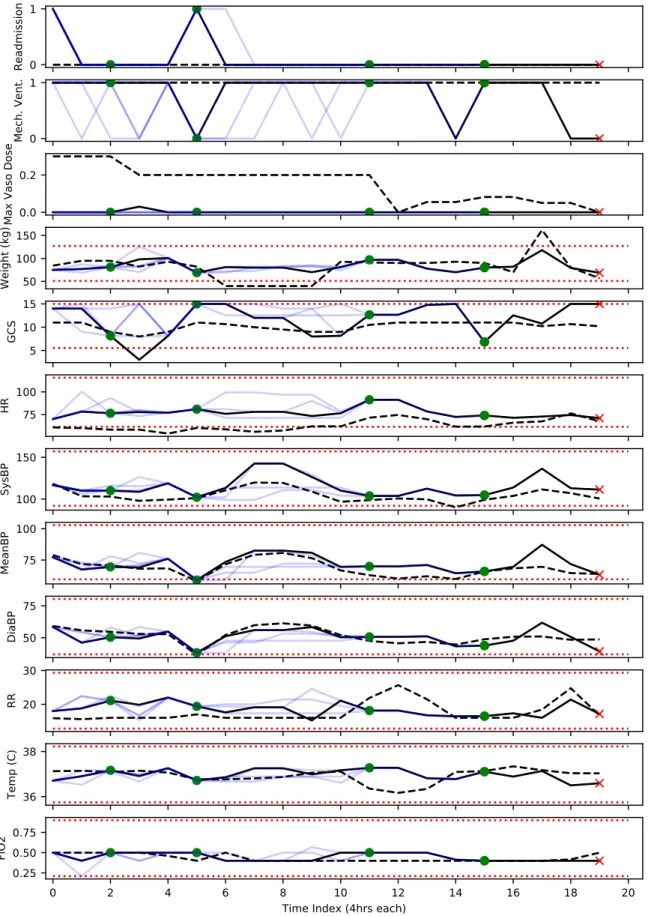
After reviewing the notes, we reviewed the counterfactual trajectories alongside the factual trajectories. We present a condensed output in Figure 7-3, consisting of a few important vital signs, and defer the full output to Figures 7-4–7-7.1 In particular, we
make the following observations
1How to read counterfactual trajectories: To visualize the counterfactual trajectories, we map the patient state back to the original space of variables. To do so, we used the median of each feature in each cluster (across the entire dataset), though this is not entirely reliable, as can be seen by comparing the black solid lines (the median values for the corresponding state in k-means) with the black dotted lines, which indicate the true values of each variable. This mismatch is discussed further in Section 7.5. To read the trajectories, note that the observed trajectory is given in black, and the counterfactuals are given in light blue, with both derived from the medians (for each feature) of their respective states. Black dotted lines indicate the patient state without using k-means clustering. Red crosses and green dots both indicate the end of the trajectory, as well as the outcome, with green indicating 90-day survival and red indicating a lack thereof. Grey circles indicate no outcome in the counterfactual. Red dotted lines indicate the middle 95% across all patients, in the original data prior to k-means.
• No basis (in medical record) for proposed actions: Recall that the patient was in fluid overload due to congestive heart failure and capillary leakage, which were themselves the result of the adjacent lung mass. The optimal approach in this setting is to carefully reduce the cardiac afterload using diuretics and anti-hypertensives, as well as drainage of the pleural e⇤usion. Thus, while vasopressors and fluids are not grossly counter-indicated, they would have the opposite e⇤ect — increasing the work of the heart because they increase cardiac afterload, eventually resulting in worsening of the patients clinical status. Thus, while in the early admission period it is not unreasonable to provide vasopressors and fluids to maintain vital signs, there is a clinical trade-o⇤, and there is no support in the medical record for giving maximum dose of vasopressors in the early stages, present in several of the counterfactual trajectories.
• Consequences of proposed actions are not reflected in CF trajectories: As noted, the alternative policy gives the maximum dose of vasopressers early on. However, the first 12 hours (first 3 time periods) look almost identical in the counterfactuals to the actual trajectory, and do not reflect the expected e⇤ect of additional vasopressors on blood pressure and other vital signs. In particu-lar, maximum dose of vasopressors should have resulted in a significant blood pressure response, which is not evident in these counterfactual trajectories.
• The anticipated outcomes are not credible given medical record: Most glar-ingly, the anticipated outcomes (discharge from the ICU and 90-day survival) are not credible given what we know about the patient from their medical record. For instance, the first counterfactual trajectory ends in 8 hours (with subsequent 90-day survival). That stands in contrast to what we know from the medical record, that the death of this patient was due to irreversible lung damage caused by Stage IIIA lung cancer and pneumonia, neither of which would have been resolved by this treatment.
Our review suggests an important possible limitation of the underlying learned MDP and policy. Important features (such as the underlying infection and lung cancer
in this case) are not included in the model, but could reasonably impact both the outcome of the patient as well as the treatment decisions of clinicians. This issue also arises in a second trajectory that we randomly sampled (not shown here), in which the clinical notes indicated that the patient died from complications due to pre-existing Hodgkin Lymphoma and treatment in the ER (prior to admission to the ICU) which triggered respiratory failure and irreversible lung injury. The counterfactuals all indicated 90-day survival, contradicting the clinical notes which suggest that by the time the patient entered the ICU, nothing more could be done.
Page 88: Insert Figure 0-1, which becomes Figure 7-4 for the revision.
Page 88-91: Replace the four figures (currently 7-3 through 7-6) with the Figures 0-2 through 0-5 in this errata.
Page 92, “Specification of states”, 2nd to last sentence: another randomly selected patient
the same patient as above
Page 93: Replace Figure 7-7 with Figure 0-6 from this errata. Page 94, Table 7.3: Replace values as follows
Train: 89.21, (87.34, 90.86) Train (Soft): 86.01, (83.84, 87.50) Train: 89.68, (88.08, 91.11) Train (Soft): 85.32, (83.74, 86.52)
Figure 0-1: Five counterfactual trajectories (for selected features), two of which end at t = 15. See description in the main text for how to read counterfactuals. HR: heart rate. BP: blood pressure. FiO2: fraction of inspired oxygen. SpO2: Peripheral
Figure 0-2: Example Trajectory including all features (Part 1/4). See description in the main text.
Figure 0-3: Example Trajectory including all features (Part 2/4). See description in the main text.
Figure 0-4: Example Trajectory including all features (Part 3/4). See description in the main text.
Figure 0-5: Example Trajectory including all features (Part 4/4). See description in the main text.
Figure 0-6: Comparison of the imputed value for each cluster) and the actual values for
Acknowledgments
It is a blessing to get to work on hard, interesting, and meaningful problems, and I cannot possibly thank all the people who have supported me along the way.
First and foremost, I am grateful for the love and support of my parents (Tom and Carla) and my siblings (Sarah, Aidan, Matthew, and Aaron). Thank you for being with me through everything, and know that I’ll always be there for you.
I’ve been blessed with and supported by more friends than I can mention here, so I’ll just pick one: Tim Chin, thanks for being a true friend and fellow adventurer in life. I wouldn’t have gotten here today without you.
To everyone in the Clinical ML group: I couldn’t have imagined a more welcoming, kind, and fun group of people with whom to spend an inordinate amount of time. You laugh at my jokes, tolerate my spontaneous and rambling musings on all things, and I couldn’t ask for more than that. Special thanks to Fredrik D. Johansson, for putting up with my research-related mood swings, being a mentor in all things causal inference, and above all for being a friend.
Naturally, I would also like to thank my advisor, David Sontag. Thank you for your commitment to working on problems that matter, for encouraging me when I needed encouragement, for pushing me onwards when I needed to be pushed, and above all for your genuine care for me and the rest of your students.
Contents
1 Introduction 11
1.1 Reinforcement Learning in Healthcare: A Challenging Task . . . 11
1.2 Motivation: Debugging Policies and Models . . . 13
1.3 Counterfactual Policy Introspection . . . 14
1.4 Structure of this Thesis . . . 20
2 Background 23 2.1 Causal Inference from Observational Data . . . 24
2.1.1 Motivating Example: Binary Treatments . . . 24
2.1.2 Dealing with Observational Data . . . 26
2.1.3 ATE, CATE, and ITE . . . 26
2.1.4 Extension to Dynamic Treatment Policies . . . 28
2.2 Model-Based Reinforcement Learning . . . 28
2.2.1 Markov Decision Processes (MDPs and POMDPs) . . . 29
2.2.2 Policy Iteration Algorithm . . . 31
2.2.3 Off-Policy Evaluation (OPE) . . . 32
2.3 Structural Causal Models and Counterfactuals . . . 35
2.3.1 Structural Causal Models (SCMs) . . . 36
2.3.2 Interventional vs. Counterfactual Distributions . . . 36
2.3.3 Non-Identifiability of Binary SCMs . . . 38
3 Counterfactual Decomposition of Reward 41
3.1 Viewing MDPs and POMDPs as SCMs . . . 41
3.2 Counterfactual Decomposition of Reward . . . 43
3.2.1 Model-Based OPE as CATE Estimation . . . 43
3.2.2 Counterfactual OPE as ITE Estimation . . . 44
4 Gumbel-Max SCMs for Categorical Variables 49 4.1 Non-Identifiability of Categorical SCMs . . . 50
4.2 Counterfactual Stability Property . . . 52
4.3 Gumbel-Max SCMs Satisfy Counterfactual Stability . . . 53
4.4 Intuition: Connection to Discrete Choice Models . . . 54
4.5 Appendix: Proofs . . . 57
5 SCMs with Additive Noise for Continuous Variables 59 6 Illustrative Applications with Synthetic Data 61 6.1 Building Intuition: 2D Gridworld . . . 61
6.1.1 Simulator Setup . . . 62
6.1.2 Generating Counterfactual Trajectories . . . 63
6.1.3 Decomposition of Reward via Counterfactuals . . . 65
6.1.4 Addendum: Counterfactual vs. Model-Based Trajectories . . . 66
6.2 Illustrative Example: Sepsis Management . . . 70
6.2.1 Setup of Illustrative Example . . . 71
6.2.2 Off-Policy Evaluation Can Be Misleading . . . 72
6.2.3 Identification of Informative Trajectories . . . 72
6.2.4 Insights from Examining Individual Trajectories . . . 73
6.2.5 Addendum: Impact of Hidden State . . . 74
7 Real-Data Case Study: Sepsis Management 79 7.1 Replicating Komorowski et al. (2018) . . . 80
7.2 Off-Policy Evaluation with WIS . . . 82
7.4 Inspection of Counterfactuals using the Full Medical Record . . . 84 7.5 Challenges and Lessons Learned . . . 92
Chapter 1
Introduction
1.1
Reinforcement Learning in Healthcare: A
Chal-lenging Task
There is a long tradition of using data to improve healthcare and public health, from randomized trials to test the efficacy of new drugs, post-market surveillance for adverse drug interactions, and the practice of epidemiology more broadly, e.g., the use of observational studies to understand the public health impact of everything from cigarettes to air pollution. Over the past decade in the United States, there has also been an ever-expanding amount of raw healthcare data, driven by the rapid adoption of electronic medical records (EMRs). As the available data has expanded, so have the ambitions of some segments of the research community, fuelled by the hope that larger and richer datasets can lead to breakthroughs in personalized medicine.
With that in mind, there has been a growing interest in the application of machine learning to healthcare, not only for diagnostic purposes (e.g., image processing in radiology and pathology), but also for learning better treatment policies, tailored to individual patients. This requires solving two closely related subproblems: First, how to learn a policy from observational (that is, retrospective) data, and second, how to evaluate it.
policy1 is required, several recent papers have used techniques from reinforcement learning (RL) to try and learn optimal policies for treating everything from sepsis (Raghu et al., 2017, 2018; Komorowski et al., 2018; Peng et al., 2018) to HIV (Parbhoo et al., 2017) and epilepsy (Guez et al., 2008). This is a challenging task, in ways that are quite different from modern success stories in reinforcement learning, such as achieving super-human performance at board games (Silver et al., 2018). The latter is a task that can be perfectly simulated, allowing for the (massive-scale) exploration and direct evaluation of different policies in a deterministic setting. In contrast, medicine is a stochastic, partially observable environment where direct experimentation by an algorithm would not be tolerable. As a result, we cannot simply try many policies and see if they work, but need to infer how a new policy would perform, using data collected under an older, different policy. In the RL literature, this is known as off-policy evaluation.
Of course, researchers in RL are not the first to have encountered this challenge. The evaluation of dynamic treatment policies (using observational data) is a well-studied causal inference problem in epidemiology and biostatistics, which is generally addressed with the application of g-methods, first introduced by Robins (1986). Lodi et al. (2016) and Zhang et al. (2018) are two recent examples, using g-methods to eval-uate HIV treatment and anemia management strategies respectively. The techniques used in RL to evaluate novel treatment policies have much in common with these techniques, such as modelling the environment directly or re-weighting the observed data, as discussed in Chapter 2.
Quantitative evaluation is nonetheless fraught with difficulties that no mathemat-ical method can address without making assumptions. For instance, if important variables are not measured (such as confounding variables, discussed in Section 2.1), then quantitative evaluation can give misleading results. These and other challenges, such as small effective sample sizes and miss-specification of reward, are discussed at length in Gottesman et al. (2019a).
1A dynamic treatment policy is one which takes intermediate outcomes into account, like stopping
Finally, a wealth of data exists in settings (e.g., EMRs, mobile health) that are not curated by any means, and are certainly not designed primarily for research purposes. This complicates matters further, and stands in contrast to research done with curated data registries, such as the US Renal Data System, used in Zhang et al. (2018), or sequentially randomized trials, such as the Strategic Timing of AntiRetroviral Treatment (START) trial, analyzed in Lodi et al. (2016).
1.2
Motivation: Debugging Policies and Models
Quantitative evaluation of policies can therefore be misleading for any number of reasons: There may exist unmeasured confounding in the dataset, the reward function (that is, the objective to be optimized) may be poorly specified, or there may not exist sufficient samples to evaluate policies that diverge too much from existing practice. Creating more robust methods for off-policy evaluation is an area of active research (Gottesman et al., 2019b; Liu et al., 2018; Kallus & Zhou, 2018), but a fundamental uncertainty remains.
Moreover, it may be difficult to inspect a policy directly, to determine whether or not it seems reasonable: In contrast to the epidemiological studies mentioned earlier (Zhang et al., 2018; Lodi et al., 2016) which pre-specify a dynamic policy to evaluate based on domain knowledge, it is not always clear what a reinforcement-learned policy is doing. In Raghu et al. (2017), for instance, the policy is parameterized by a neural network, and in Komorowski et al. (2018), the policy associates an action with each of 750 patient state clusters derived via k-means clustering.
With that in mind, consider the following hypothetical: Suppose that you have the power to change medical practice, and are given a complex policy which is claimed (e.g., due to off-policy evaluation) to perform far better than existing clinical guide-lines. How might you proceed? Given the challenges of retrospective evaluation, you might want to test the policy prospectively, perhaps using a randomized trial. But before you did that, you would want to better understand the policy, before investing a large amount of time and money in a gold-standard evaluation. In essence, you may
wish to search for ‘bugs’ in the policy (like a tendency to take dangerous actions), or the model used to generate it (like the omission of a critical input), and iterate until you are confident that the policy has learned something reasonable.
There are a variety of ways you could do this, even if the policy is too complex to be interpretable directly. For instance, a physician might randomly select some real pa-tients, pull up their full medical record, and compare the actions taken by the doctors to the recommendations of the learned policy, to see if they seem reasonable. Jeter et al. (2019) perform such an analysis in their critique of Komorowski et al. (2018), highlighting a sepsis patient where the learned policy makes a counter-intuitive deci-sion to withhold treatment during a critical hypotensive episode. However, manual inspection of randomly selected trajectories may be inefficient, and difficult to inter-pret without more information: If we are to discover new insights about treatment, shouldn’t there be some disagreement with existing practice?
This poses two problems: First, how do you surface the ‘rationale’ of a policy? In an ideal world, we could elicit a justification for each action. We refer to this as the challenge of policy introspection. Second, supposing that you could elicit these justi-fications en masse across all trajectories, how would you select the most interesting case examples for manual inspection?
1.3
Counterfactual Policy Introspection
In this thesis, we give a procedure that uses counterfactual trajectories to address both of these questions, and refer to this procedure as counterfactual policy introspec-tion. Given a policy and a learned model of the environment, we provide a post-hoc method to generate counterfactual trajectories for each observed (or ‘factual’) tra-jectory, which attempt to describe what the model expects would have happened, in hindsight, if that policy had been used. We note that this is most useful in ap-plications that already require the learning of a model of the environment, such as in model-based reinforcement learning. We can then compare counterfactual trajec-tories with observed trajectrajec-tories, potentially with additional side-information (e.g.,
chart review in the case of a patient) so that domain experts can “sanity-check” a policy and the model used to learn it. In a way that we make precise in Section 3.2, if these counterfactuals are obviously wrong, then it provides evidence that the learned model of the environment is flawed.
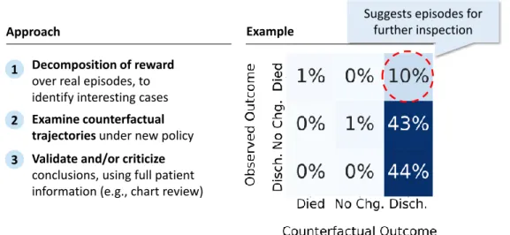
Thus, our end-to-end procedure for ‘debugging’ models and policies is as fol-lows, illustrated in Figure 1-1: First, once we have counterfactual trajectories for each observed trajectory, we can highlight episodes where there are surprisingly large differences between the factual and counterfactual outcomes. Second, we can then perform manual examination of the observed and counterfactual trajectories, to iden-tify disagreements between the learned policy and existing practice, and to try and understand the rationale for them. Critically, because these are real patients, we can also go look for additional information to ‘kick the tires’ of the counterfactual conclusions. Finally, we can use our findings to iterate on the model and policy. For instance, looking at the medical record may suggest new variables to include in our model of the environment, at which point we can repeat the process again.
1 Decomposition of reward
over real episodes, to identify interesting cases
Approach
2 Examine counterfactual trajectories under new policy 3 Validate and/or criticize
conclusions, using full patient information (e.g., chart review)
Example
Suggests episodes for further inspection
Figure 1-1: Conceptual overview of our approach: First, counterfactual trajectories are generated for all observed trajectories, and are then used to guide manual inspec-tion. The figure on the right is taken from a synthetic example of sepsis management in Section 6.2, and highlights patients who died, but who would have allegedly lived in the counterfactual.
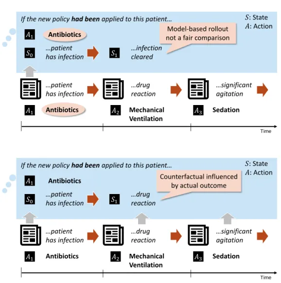
We stress that these counterfactuals are conceptually distinct from the simulation of new trajectories using a learned model of the environment. In particular, we don’t want to know what the model believes might generally occur under a different policy: We want to know what would have been different in a specific trajectory. In Figure 1-2 we give a conceptual example of this distinction, in line with the medical use case described above. In this example, we imagine an observed trajectory where the patient had a rare, adverse reaction to an antibiotic. In a model-based simulation (or ‘roll-out’), what might occur? Since the reaction is rare, then a model-based simulation might reasonably predict the most common outcome for patients in general (that the infection is cleared). Naturally, this does not satisfy our intuition for what would have happened to this specific patient (we already know!), but a model-based simulation is not designed to satisfy this intuition. A counterfactual trajectory, on the other hand, is designed to take into account what actually occurred to this patient, in a way that will be made precise in Section 2.3.
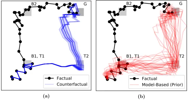
Moreover, counterfactual trajectories incorporate strictly more information about the observed trajectory, and thus exhibit less variance than a freshly simulated tra-jectory from a model. This is illustrated in a toy 2D grid-world setting in Figure 1-3, where the counterfactual trajectories in the left-hand figure (in blue) overlap perfectly with the observed trajectory (in black) when the actions are identical, and exhibit little variability even after actions diverge. This is in contrast to the simulated tra-jectories in the right-hand figure (in red), which borrow no information from the observed trajectory, and thus are different from the beginning, even under identical actions. This example is discussed in far more depth in Section 6.1.2.
Returning to our motivating example of evaluating a complex treatment policy, it is worth repeating that these counterfactuals may be obviously wrong, es-pecially if we go to the medical record and use additional side information to check it against our intuition. This is a feature, not a bug, of our approach: In a setting where the model used for counterfactual evaluation is the same model that was used to train the policy, this can be used to confirm that suspicious actions (e.g., with-holding treatment) are based on a faulty model of the world, versus a real insight
If the new policy had been applied to this patient… Antibiotics …patient has infection 𝑆0 𝐴1 Time Antibiotics Mechanical Ventilation Sedation …patient has infection …drug reaction …significant agitation 𝑆: State 𝐴: Action 𝐴1 𝐴2 𝐴3 …infection cleared 𝑆1 Model-based rollout not a fair comparison
If the new policy had been applied to this patient…
Antibiotics …patient has infection 𝑆0 𝐴1 Time Antibiotics Mechanical Ventilation Sedation …patient has infection …drug reaction …significant agitation 𝑆: State 𝐴: Action 𝐴1 𝐴2 𝐴3 𝑆1 …drug reaction Counterfactual influenced by actual outcome
Figure 1-2: In this example, we imagine an observed trajectory where the patient had a rare, adverse reaction to an antibiotic. In a model-based roll-out, even if the trajectory is started in the same state, with the same initial action, it is unlikely that all model-based roll-outs will include this adverse event. Thus, the model-based roll-out is harder to critique: Perhaps the model is correct, and this patient just got unlucky. A counterfactual trajectory, on the other hand, is designed to isolate differences which are due to differences in actions.
into the best treatment.2 In a model-based simulation, by contrast, this is difficult to ascertain: Was the model wrong, or was this patient just one of the unlucky ones?
However, towards generating these counterfactual trajectories, we have to deal with a fundamental issue of non-identifiability: As we show in Section 4.1, even with
G
B1, T1
B2
T2
Factual
Counterfactual
(a)G
B1, T1
B2
T2
Factual
Model-Based (Prior)
(b)Figure 1-3: A visual example of how counterfactuals isolate differences that are due solely to divergence in actions from the factual, taken from Section 6.1.2. The black line represents an observed trajectory, whereas the blue and red lines represent counterfactual trajectories and model-based simulations, respectively
an infinite amount of interventional data, there are multiple structural causal models (as introduced in Section 2.3) which are consistent with with the data we observe, but which suggest different distributions of counterfactual outcomes on an individual level. This is not a new problem, and a common assumption in the binary setting to identify counterfactuals is the monotonicity condition (Pearl, 2000). However, to our knowledge, there is no analogous condition for the categorical case, as would be required to generate counterfactuals in discrete state-space models of the environment.
This motivates our main theoretical contribution, which is two-fold. First, we introduce a general condition of counterfactual stability for structural causal models (SCMs) with categorical variables and prove that this condition implies the mono-tonicity condition in the case of binary categories. Second, we introduce the Gumbel-Max SCM, based on the Gumbel-Gumbel-Max trick for sampling from discrete distributions, and demonstrate that it satisfies the counterfactual stability condition. We note that any discrete probability distribution can be sampled using a Gumbel-Max SCM; As a result, drawing counterfactual trajectories can be done in a post-hoc fashion, given
any probabilistic model of dynamics with discrete states. To conclude, we restate our main contributions, which are as follows:
1. Using Counterfactuals for Policy Introspection and Model-Checking: Our main conceptual contribution is the procedure described above, using coun-terfactual trajectories as a tool for introspection of learned policies and models. Additionally, we build on the theoretical results of (Buesing et al., 2019) in Sec-tion 3.2 to note that the expected counterfactual reward over all factual episodes (if the SCM is correctly specified) is in fact equal to the expected reward using freshly simulated trajectories. In this way, if counterfactual conclusions are in-correct on their face, it casts suspicion on the learned model of dynamics used in the first place, and any quantitative estimate of reward (as derived through e.g., the parametric g-formula, discussed in Section 2.1) that it yields.
2. Counterfactual Stability and Gumbel-Max SCMs: Our main theoreti-cal contribution is twofold: First, we introduce the property of counterfactual stability for SCMs with categorical variables, and prove that this condition im-plies the monotonicity condition (Pearl, 2000) in the case of binary categories. Second, we introduce the Gumbel-Max SCM, a general SCM for categorical vari-ables which we prove to satisfy the counterfactual stability condition. We note that any discrete probability distribution can be sampled using a Gumbel-Max SCM; As a result, drawing counterfactual trajectories can be done in a post-hoc fashion, given any probabilistic model of dynamics with discrete states.
3. Application to a Real-World Setting: In addition to a series of synthetic examples, we replicate the work of Komorowski et al. (2018) in learning a pol-icy for sepsis management using EMR data. We apply counterfactual polpol-icy introspection with the assistance of a domain expert (in this case, a clinician), including the review of specific counterfactual trajectories using the full medical record as side information.
1.4
Structure of this Thesis
∙ Background (Chapter 2): We review the interrelated problems of learning and evaluating a dynamic policy, drawing connections between the literature on causal inference and model-based reinforcement learning. We also review the concepts necessary for generating counterfactuals, such as structural causal models. We draw a distinction between counterfactual and interventional distri-butions, and highlight both the inherent non-identifiability of counterfactuals, as well as the monotonicity assumption used to identify them in the binary case.
∙ Counterfactual Decomposition of Reward (Chapter 3): We begin by demonstrating how common causal models assumed in the RL literature (MDPs and POMDPS) can be cast as structural causal models. We further discuss the connection between counterfactual estimates of rewards and notions like CATE and ITE in the causal inference literature. We conclude by building on the the-oretical results of (Buesing et al., 2019) in Section 3.2 to note that the expected counterfactual reward over all factual episodes (if the SCM is correctly specified) is in fact equal to the expected reward using freshly simulated trajectories.
∙ Gumbel-Max SCMs for Categorical Variables (Chapter 4): With the motivation from Chapter 3 in mind, in this chapter we introduce our core the-oretical contributions. First, we introduce the property of categorical stability as a categorical analog of the montonicity assumption. Then, we introduce and motivate the Gumbel-Max SCM by proving that it satisfies this property. We also highlight connections to the discrete choice literature, which are useful for building intuition around the counterfactual stability condition.
∙ SCMs with Additive Noise for Continuous Variables (Chapter 5): In this brief chapter, we highlight some possible approaches for developing general SCMs for continuous variables, by examining common continuous state-space models in RL and giving an SCM which is consistent with their formulation.
intuition, we demonstrate the use of counterfactual trajectories in two idealized environments: A 2D grid-world and an illustrative simulator of sepsis. The for-mer builds intuition for how counterfactual inference works in SCMs, while the latter demonstrates our proposed use of counterfactuals for policy introspection.
∙ Real-Data Case Study: Sepsis Management (Chapter 7): In this chap-ter, we replicate the work of Komorowski et al. (2018) using real EMR data to learn a policy of sepsis management, and we apply our proposed methodol-ogy to perform introspection of the resulting policy. Most notably, we use the full medical record and the help of a clinician to examine counterfactuals for a particular trajectory, and discuss our insights from this exercise in Section 7.4.
Chapter 2
Background
In this chapter, we lay out the necessary background for the later chapters. Broadly speaking, we start by discussing the central problem of learning how to act from data. This is intrinsically a causal question: We would like to claim that if we acted in a particular way, this would bring about a particular outcome. Thus, in Section 2.1, we discuss some basic principles of causal inference, starting with the simplest case of estimating the effect of a binary action from interventional data (as in a randomized control trial), before moving on to techniques used to estimate the effect of dynamic treatment regimes from observational data. We highlight in particular some general classes of methods: Those which model the causal relationships directly, those which rely on re-weighting the data, and those which combine the two approaches.
With this background in hand, we turn to the problem of learning a policy from data, and highlight methods used in the reinforcement learning (RL) community for doing so in Section 2.2. We draw an explicit connection to the literature on dynamic treatment regimes, noting that RL methods can be viewed as assuming a particular causal graph with a certain Markov structure. With this assumption in mind, we discuss a basic method for learning an optimal policy, known as Policy Iteration, which falls under the general class of RL methods which are ‘model-based’, in that they assume access to a model of the environment. We then discuss two approaches in the RL literature for evaluating policies that are different from the one that generated the data, a problem known as off-policy evaluation: The first of
these methods, known as model-based off-policy evaluation (MB-OPE) bears some similarity to the g-formula used in the literature on evaluating dynamic treatment regimes. The second method is a re-weighting method, which is similar to inverse propensity (IP) weighting methods, another set of g-methods.
Finally, we introduce the notion of counterfactuals in Section 2.3, where we formal-ize the distinction between interventional questions, like ‘what will happen if I apply policy X’, and counterfactual questions, like ‘what would have happened if I had ap-plied policy X, given that I apap-plied policy Y and observed outcome Z’. To do so, we introduce the mathematical framework of structural causal models, and highlight the challenges inherent in estimating counterfactuals, which are by definition never observed. We note that this is a different (and strictly more challenging) problem than the usual causal inference question, because it deals with individual-level coun-terfactuals (analogous to the individual treatment effect), instead of population-level causal effects (analogous to the conditional average treatment effect).
We refer the reader to several reference on the above topics for more detail, in lieu of attempting to reproduce the entirety of these fields within the confines of this thesis. In particular, we recommend Hernan & Robbins (2019) for an overview of causal inference with dynamic treatment regimes, and Pearl (2009); Peters et al. (2017) for an overview of causal graphs and structural causal models. For a general overview of reinforcement learning, we recommend Sutton & Barto (2017).
2.1
Causal Inference from Observational Data
2.1.1
Motivating Example: Binary Treatments
Suppose that we want to evaluate the causal effect of a binary action, such as taking an antibiotic, on a binary outcome, such as whether or not an infection is cleared. Let 𝑇 ∈ {0, 1} represent the action (whether or not we gave the treatment), and let 𝑌 ∈ {0, 1} represent the outcome. Suppose we also have access to covariates / features 𝑋 which describe potential confounding factors, so-called because they
influence both the treatment decision and the outcome. For any given individual, we can use 𝑌1 and 𝑌0 to represent the potential outcomes (Morgan & Winship, 2014) under the treatment and control respectively, of which we only observe one of the two, e.g., 𝑌 = 𝑌1𝑇 + 𝑌0(1 − 𝑇 ). We can also denote this set-up using a causal graph, a directed acyclic graph (DAG) which encodes the causal relationships between random variables (Pearl, 2009). In this case, the corresponding DAG is given in Figure 2-1, with arrows that represent the causal relationships between variables.
𝑌 𝑇
X
Figure 2-1: Causal graph corresponding to the motivating example of a binary treat-ment and binary outcome
In this example, we might be interested in the average treatment effect (ATE), which can be denoted by
𝜏 = E[𝑌 |𝑑𝑜(𝑇 = 1)] − E[𝑌 |𝑑𝑜(𝑇 = 0)],
where the 𝑑𝑜(·) operator is used to indicate an intervention. The 𝑑𝑜(·) operator is reviewed in (Pearl, 2009), and is accompanied by the rules of do-calculus, which give us a set of conditions which specify when (and how) it is possible to obtain causal relationships, like P(𝑌 |𝑑𝑜(𝑇 = 𝑡)), from observed conditional relations like P(𝑌 |𝑇 = 𝑡). Intuitively, the ATE corresponds to the expected difference in outcome between two policies, where we treat everyone E[𝑌 |𝑑𝑜(𝑇 = 1)] or we treat no one 𝐸[𝑌 |𝑑𝑜(𝑇 = 0)]. In the simplest case, if the treatment assignment is randomized such that P(𝑇 |𝑋) = P(𝑇 ), then we have the equivalence E[𝑌 |𝑑𝑜(𝑇 = 𝑡)] = E[𝑌 |𝑇 = 𝑡]. For instance, in an ideal randomized control trial with full compliance, we could estimate the causal effect by simply looking at the difference in outcome between the treatment and control groups.
2.1.2
Dealing with Observational Data
It should be noted that causal inference requires assumptions, which are often not empirically verifiable. For instance, if treatment assignment is not randomized, as is typical for observational data, a common approach is to first make the assumption of no unmeasured confounding: That is, we assume that we observe, through 𝑋, all of the variables which impact both the treatment and the outcome. We refer the reader to a variety of references (Hernan & Robbins, 2019; Pearl, 2009; Morgan & Winship, 2014; Imbens & Rubin, 2015) for a more comprehensive treatment of the topic, but we will briefly highlight three broad approaches, which have analogs in the reinforcement learning literature.
∙ First, we can model the conditional relationships directly, by estimating P(𝑌 |𝑋, 𝑇 ), which is equivalent to P(𝑌 |𝑋, 𝑑𝑜(𝑇 )) under the assumption of no unmeasured confounding, and use this to calculate P(𝑌 |𝑑𝑜(𝑇 )) = ∫︀
P(𝑌 |𝑋, 𝑇 )P(𝑋)𝑑𝑥 by marginalizing over 𝑋. This is known as standardization in epidemiology.
∙ Second, we can re-weight the data to create a psuedo-population that approxi-mates the results of a randomized trial. For instance, we might use an estimate of the treatment probability P(𝑇 |𝑋), known as the propensity score, and use this to re-weight our observations (Rosenbaum & Rubin, 1983), or stratify into sub-populations with similar propensity (Rubin & Rosenbaum, 1984). The more general form of this approach (discussed below) is known as inverse probability (IP) weighting in epidemiology.
∙ Finally, we can combine the two approaches above to develop doubly-robust esti-mators (Bang & Robins, 2005), which provide asymptotically correct estimates if we can correctly estimate either P(𝑌 |𝑋, 𝑇 ) or P(𝑇 |𝑋).
2.1.3
ATE, CATE, and ITE
So far, we have implicitly focused on a very simple decision-making problem, by focusing on the estimation of the ATE. In effect, this corresponds to evaluating the
difference in the expected outcome between two policies: ‘Treat everyone’ and ‘treat no one’. In the notation of potential outcomes, introduced in Section 2.1.1, the ATE corresponds to the quantity
𝜏 = E[𝑌1− 𝑌0]
We can refine this further by investigating the conditional average treatment effect (CATE), which conditions on a specific subpopulation 𝑋, and can be denoted by the quantity
𝜏𝑥 = E[𝑌1− 𝑌0|𝑋]
In the causal graph given in Figure 2-1, this can (in principle) be estimated directly using regression models ˆ𝑓 (𝑋, 𝑇 ) ≈ E[𝑌 |𝑋, 𝑇 ] since 𝑃 (𝑌 |𝑋, 𝑑𝑜(𝑇 )) = 𝑃 (𝑌 |𝑋, 𝑇 ) in this case. How does this relate to learning a policy? In this simple setting, learning a policy follows naturally from evaluating the effect of the binary treatment. For instance, once we have learned the CATE, we can devise a policy which treats each patient (with covariates 𝑋) based on the sign of the estimated CATE ˆ𝜏𝑥.
Note that there is a conceptual distinction between the CATE and what we will refer to as the individual treatment effect (ITE), which is simply the difference in potential outcomes, denoted for an individual 𝑗 by
𝜏𝑖𝑡𝑒(𝑗) = 𝑌1(𝑗)− 𝑌0(𝑗)
Unlike the ATE and CATE, this represents a statement about a specific individual, versus an expectation over a population. This can be a source of confusion when it comes to the use of counterfactual language: It is not uncommon to estimate the CATE and refer to this as a counterfactual or to refer to the CATE as the ITE (see Shalit et al. (2016) and discussion in Appendix B of Liu et al. (2018)).
Note that in this thesis, we will reserve the language of counterfactuals and coun-terfactual inference to refer to individual-level quantities, like 𝑌0(𝑗), 𝑌1(𝑗).
2.1.4
Extension to Dynamic Treatment Policies
Many of the methods which were originally developed for the simple setting described above do not work (when applied naively) to the setting where we wish to evaluate a dynamic treatment. In this setting, our initial action may have some intermediate effect which influences our choice of later actions, and so on. Robins (1986) introduced a class of general methods for adjustment in this setting, which are referred to g-methods in the dynamic treatment regime literature. Among these, we highlight two methods which are analogs to those discussed previously:
∙ First, the g-computation algorithm formula, typically referred to as the g-formula, is a generalization of the standardization approach given in Section 2.1.2. Sim-ply put, the conceptual approach is to estimate the outcome under a specific policy by simulating from a model of the overall environment. The g-formula is widely used in epidemiology, where it is referred to as the parametric g-formula when it involves fitting a parametric model of the environment. For instance, Lodi et al. (2016) use this approach to evaluate a policy for HIV treatment, and Zhang et al. (2018) use it to evaluate a strategy for anemia management.
∙ Second, the class of inverse probability (IP) weighting methods, which gener-alize the re-weighting methods discussed previously, such as propensity score re-weighting (Rosenbaum & Rubin, 1983). See (Hernan & Robbins, 2019) for a more in-depth discussion, including the combination of IP weighting methods with marginal structural models.
2.2
Model-Based Reinforcement Learning
With all of this in mind, we shift gears to a different set of literature, namely that of reinforcement learning (RL). In contrast to the above sections, where our focus was on evaluating a policy based on observational data, reinforcement learning has its roots in trying to learn a policy efficiently, when given the ability to experiment freely in an environment. We cannot hope to summarize all the extant techniques
that exist for learning and evaluation in RL, but instead highlight those which are relevant for future chapters, as well as for understanding where our approach fits in. Seen in relationship to the literature on dynamic treatment regimes, the reinforce-ment learning literature tends to assume a particular type of causal graph, a Markov Decision Process (MDP), which we describe in Section 2.2.1. While this assumption is shared across techniques used to learn a policy, there is a further distinction between methods which are model-based, which rely on learning to model the MDP, versus those that are ‘model-free’, in the sense that they do not model the environment di-rectly. The techniques discussed in this thesis require a model of the environment, and thus we will focus our discussion in Section 2.2.2 on a simple model-based approach to learning a policy, known as Policy Iteration.
Finally, we discuss two broad types of evaluation, which have connections to the two classes of evaluation methods discussed in the previous section: First, model-based off-policy evaluation (MB-OPE), which can be seen as a specific instance of simulation via the g-formula, and importance re-weighting methods such as weighted importance sampling (WIS), which can be seen as instances of the inverse probability weighting approach described earlier.
2.2.1
Markov Decision Processes (MDPs and POMDPs)
The reinforcement learning literature tends to assume an underlying model of the world which can be represented as having a Markov structure, meaning that the state of the world in the future is independent of the past, given the present (observable) state. This leads to a representation which is known as a Markov Decision Process (MDP). This can be relaxed by assuming that there exists an underlying Markov structure, but we may not observe it, in which case it is considered a partially observ-able Markov Decision Process (POMDP). In this section we describe these general models, as a prelude to discussing their role in both learning and evaluation.
We follow the description of Finite Markov Decision Processes (MDPs) given in Sutton & Barto (2017), to which we refer the reader for more information. In this setting, the decision-maker (or agent ) interacts with an environment at each discrete
time step. The decision maker is presented with a state 𝑆 ∈ 𝒮, and chooses an action 𝐴 ∈ 𝒜, which result in a new state 𝑆′ ∈ 𝒮 as well as a quantitative reward 𝑅 ∈ ℛ, and the process continues until an absorbing state is reached, or until a fixed time (known as a fixed-horizon MDP). These states, actions, and rewards are typically indexed by time, and follow the conditional probability distribution (CPD) that governs the MDP, and which is referred to (in this work) as the dynamics of the process:
P(𝑆𝑡+1, 𝑅𝑡|𝑆𝑡, 𝐴𝑡) (2.1)
Note that the CPD in Equation (2.1) is Markov in the sense that the next state / reward only depend on the previous state and action, hence the moniker of a Markov Decision Process. Furthermore, this CPD is often assumed to be invariant to the time index, in which case we refer to this as a homogenous MDP. Finally, when the state space 𝒮 has finite cardinality, we refer to this as a finite MDP.
The goal of the decision-maker at time 𝑡 is typically to maximize the discounted expected reward over the future states. This is typically denoted as follows1
𝐺𝑡 := ∞ ∑︁ 𝑘=0
𝛾𝑘𝑅𝑡+𝑘+1 (2.2)
In Equation (2.2), the discount factor 0 ≤ 𝛾 ≤ 1 determines the degree to which future rewards are less valuable than immediate rewards, and this notation can be used to cover episodes which have a finite horizon or terminal states, using the assumption that after the horizon or a terminal state is reached, the subsequent rewards are all zero.
Thus, the goal of the decision-maker is to choose a policy 𝜋 which maximizes the expected reward. This policy can either be deterministic, in which case 𝜋 : 𝒮 → 𝒜 maps states to actions, or stochastic, in which case 𝜋 : 𝒮 × 𝒜 → R gives a probability density or mass function over the set of possible actions for each state, such that ∑︀
𝑎∈𝒜𝜋(𝑠, 𝑎) = 1, ∀𝑠 ∈ 𝒮. With a slight abuse of notation, we will sometimes write
𝜋(𝑎|𝑠) in place of 𝜋(𝑠, 𝑎) to convey the fact that it describes a conditional probability distribution over actions.
An extension of this framework is to consider a partially observable MDP (POMDP), in which we distinguish between the true state 𝑆𝑡 and the observation 𝑂𝑡at each time step, with the assumption that the true state 𝑆𝑡 is unobserved. In this case, the generative model is augmented with the CPD P(𝑂𝑡|𝑆𝑡). In the case of a POMDP, the policy may depend on the entire history up to time point 𝑡, which is denoted as 𝐻𝑡 := {𝑂1, 𝐴1, 𝑅1, . . . , 𝑂𝑡−1, 𝐴𝑡−1, 𝑅𝑡−1, 𝑂𝑡}, such that the policy is given by 𝜋(𝑎|ℎ), with ℎ ∈ ℋ informing the action taken.
A trajectory or episode, denoted 𝜏 , is the full sequence of states, actions, and rewards, up to the terminal state or horizon. For a MDP, given a probability dis-tribution over initial states P(𝑆1) and policy 𝜋(𝑎|𝑠), the probability of any given trajectory 𝜏 = {𝑆1, 𝐴1, 𝑅1, . . . , 𝑆𝑇, 𝐴𝑇, 𝑅𝑇} is given by 𝑝(𝜏 ) = P(𝑆1) 𝑇 ∏︁ 𝑘=2 𝜋(𝐴𝑘−1|𝑆𝑘−1)P(𝑆𝑘, 𝑅𝑘|𝐴𝑘−1, 𝑆𝑘−1) (2.3)
With an analogous factorization in the case of a POMDP. Because this distribution depends on the policy 𝜋, we denote this distribution over 𝜏 by 𝑝𝜋(𝜏 ), and for any quantity which is a function of the trajectory (e.g., the total reward 𝐺), we will write
E𝜋(·) to denote the expected value over trajectories drawn from 𝑝𝜋(𝜏 ).
2.2.2
Policy Iteration Algorithm
There are a variety of techniques used to find an optimal policy in the case of a finite MDP, but for our purposes it will be sufficient to discuss the techniques used in (Komorowski et al., 2018), which use straightforward iterative optimization techniques that depend on knowledge of the MDP, which can be estimated from data.
is defined with respect to a policy 𝜋 by2 𝑣𝜋(𝑠) = E𝜋[𝐺𝑡|𝑆𝑡= 𝑠] (2.4) =∑︁ 𝑎 𝜋(𝑎|𝑠)∑︁ 𝑠′,𝑟 𝑝(𝑠′, 𝑟|𝑠, 𝑎) [𝑟 + 𝛾𝑣𝜋(𝑠′)] (2.5)
With this in hand, the policy evaluation problem is to estimate the value function for a given policy. Equation (2.5) defines a fixed point, and the following iterative update rule is known to converge to true value function
𝑣𝜋(𝑘+1)(𝑠) ←∑︁ 𝑎 𝜋(𝑎|𝑠)∑︁ 𝑠′,𝑟 𝑝(𝑠′, 𝑟|𝑠, 𝑎)[︀𝑟 + 𝛾𝑣(𝑘) 𝜋 (𝑠 ′)]︀ , (2.6)
where 𝑣(𝑘) is the value function at the 𝑘-th iteration. Initializing a random value function and applying these updates until some desired tolerance is known as the iterative policy evaluation algorithm.
Using this technique for evaluating a policy as a subroutine, the policy iteration algorithm improves the policy at each step, using the update rule given by
𝜋′(𝑎|𝑠) ← max 𝑎
∑︁ 𝑠′,𝑟
𝑝(𝑠′, 𝑟|𝑠, 𝑎) [𝑟 + 𝛾𝑣𝜋(𝑠′)] (2.7)
To summarize, policy improvement starts with a random (deterministic) policy and a randomly initialized value function, then alternates between policy evaluation and policy improvement, until it finds a stable policy. For more detail, we refer the reader to Chapters 4.1–4.3 of Sutton & Barto (2017).
2.2.3
Off-Policy Evaluation (OPE)
In the RL literature, it is commonly assumed that we are able to learn from experi-ence. That is, we can experiment with different policies until we find a policy that maximizes our expected reward. From the perspective of healthcare applications, this is analogous to assuming that we can freely run our own randomized experiments
as we go along. Evaluation in this setting (the on-policy setting) is conceptually straightforward, similar to a randomized trial.
In this thesis, we deal with the setting where this type of experimentation is not possible, e.g., for ethical and practical reasons, and we are restricted to using observational data. This type of setting is referred to in the RL literature as off-policy batch RL, to reflect that the off-policy used to generate the data (the ‘behavior’ policy) is different from the policy we wish to evaluate (the ‘target’ or ‘evaluation’ policy) and the fact that our dataset is restricted to a fixed batch of data.
Here we discuss two methods for off-policy evaluation, which have connections to the classes of evaluation methods discussed in Section 2.1:
∙ Model-based off-policy evaluation (MB-OPE) involves learning a parametric model of an underlying MDP, and then using this to estimate the value of a policy (see e.g., Chow et al. (2015); Hanna et al. (2017)), and can thus be seen as a specific instance of simulation via the g-formula.
∙ Importance sampling (IS) (Rubinstein, 1981) is the foundation for a series of techniques, such as weighted importance sampling (see e.g., Precup et al. (2000)). As discussed below, these are similar to IP weighting methods.
∙ There exist several methods for combining these approaches, whether to gen-erate doubly robust estimates of performance (Jiang & Li, 2016; Bibaut et al., 2019; Farajtabar et al., 2018), or using a mixture of IS and MB estimates (Thomas & Brunskill, 2016; Gottesman et al., 2019a).
We take a moment here to describe the form of a basic IS estimator, as well as weighted importance sampling (WIS), as they will be relevant for our later experi-mental work replicating Komorowski et al. (2018). In general, importance sampling and related approaches (IP weighting, inverse propensity weighting) take advantage of the following relationship, where 𝑝, 𝑞 are two different distributions
E𝑝[𝑌 ] = ∫︁ 𝑦 · 𝑝(𝑦)𝑑𝑦 = ∫︁ 𝑦 · 𝑝(𝑦) 𝑞(𝑦)𝑞(𝑦) = E𝑞 [︂ 𝑝(𝑦) 𝑞(𝑦)𝑌 ]︂
This is the same basic theory that underlies all the IP weighting methods discussed so far.3 Thus, given samples of a random variable from a distribution 𝑞, we can approximate the expectation under the distribution 𝑝 using the weights 𝑝(𝑦𝑖)/𝑞(𝑦𝑖) for each 𝑦𝑖, and taking a sample average E𝑝[𝑌 ] ≈ 𝑛−1∑︀ 𝑦𝑖· 𝑝(𝑦𝑖)/𝑞(𝑦𝑖)
In an RL context, we want to estimate the expected reward of an evaluation policy 𝜋𝑒, given data sampled from an MDP under a behavior policy 𝜋𝑏. In this case the importance ratio is straightforward. Examining the probability of any given trajectory, given in Equation 2.3, we note that all the terms cancel in the importance sampling ratio, except for those which involve the policy. Thus, the importance sampling ratio is given by the following, where we use 𝜌1:𝑇 to denote the importance sampling ratio over 𝑇 time steps
𝜌1:𝑇 = 𝑇 ∏︁ 𝑖=1 𝜋𝑒(𝑎𝑡|𝑠𝑡) 𝜋𝑏(𝑎𝑡|𝑠𝑡)
Using importance sampling, we can get an unbiased and consistent estimator of the reward under the evaluation policy using E𝜋𝑒[𝐺] ≈ 𝑛
−1∑︀ 𝑖𝜌
(𝑖)𝐺(𝑖), where we drop
the subscript on 𝜌, use the superscript to indicate observed trajectories, and write 𝐺 as the total discounted reward. However, in practice the IS estimator can exhibit high variance, especially if some actions are rare under the behavior policy (such that 1/𝜋𝑏(𝑎𝑡|𝑠𝑡) is very large).
Weighted importance sampling is an alternative estimator which exhibits much lower variance, albeit at the cost of introducing some bias.4 The weighted importance sampling estimator performs a weighted average instead of a simple average, and is given by ∑︀ 𝑖𝜌 (𝑖)· 𝐺(𝑖) ∑︀ 𝑖𝜌(𝑖) ,
It is important to note that all variants of importance sampling are subject to the
3Note that this relationship is only well-defined if 𝑝(𝑦) > 0 =⇒ 𝑞(𝑦) > 0. This condition goes by
various names depending on the field: In probability theory, it is referred to as absolute continuity. In the context of inverse propensity weighting, it is referred to as overlap or positivity. In the context of reinforcement learning, it is referred to as coverage.
4Weighted importance sampling is still consistent, in the sense that it converges to the correct
same assumptions as any other causal analysis. That is, we typically need to estimate the behavior policy from data, and if there is some unmeasured confounding factor which cause our estimates of the behavior policy 𝜋𝑏 to be incorrect, then our IS or WIS estimates will also be incorrect. This well-known fact is demonstrated in our synthetic experiments in Section 6.2.2.
2.3
Structural Causal Models and Counterfactuals
When we discussed binary treatments in Section 2.1.3 we discussed potential outcomes 𝑌1, 𝑌0. In that setting, we observe one of these, but the other is unknown, representing the theoretical counterfactual outcome. In many applications of causal inference, we wish to estimate some general effect of an intervention, such as the conditional average treatment effect E[𝑌1− 𝑌0|𝑋] (e.g., Schulam & Saria, 2017; Johansson et al., 2016), because this represent general knowledge about interventions that we can apply to future patients. But we do not particularly care about e.g., estimating 𝑌0 given 𝑌1 for a particular patient that we have already treated, because we cannot go back in time and take a different action.
In a sense that we will make precise in Section 2.3.2, the CATE is a property of the interventional distribution of 𝑌 , describing how 𝑌 changes in response to interventions on other variables (in this case, 𝑇 ). However, we would like to go a step beyond this, as described in Section 1.3. We would like to take into account what actually happened to get a more precise estimate of what would have happened had a different action (or set of actions) been taken. This is a counterfactual question. In essence, we want to estimate something that is conceptually akin to the individual treatment effect 𝑌1− 𝑌0, rather than just the CATE.
To do so, we need to introduce the mathematical formalism of structural causal models, which give a well-defined answer to these questions. In Section 2.3.1 we intro-duce the general framework, in Section 2.3.2 we formalize the conceptual distinction between interventional and counterfactual distributions, and in Sections 2.3.3-2.3.4 we discuss the fundamental challenge of non-identifiability, as well as some assumptions
that make identification possible in the binary case.
2.3.1
Structural Causal Models (SCMs)
As promised, we review the concept of structural causal models, and encourage the reader to refer to Pearl (2009) (Section 7.1) and Peters et al. (2017) for more details. A word regarding notation: As a general rule throughout, we refer to a random variable with a capital letter (e.g., 𝑋), the value it obtains as a lowercase letter (e.g., 𝑋 = 𝑥), and a set of random variables with boldface font (e.g., X = {𝑋1, . . . , 𝑋𝑛}). Consistent with Peters et al. (2017) and Buesing et al. (2019), we write 𝑃𝑋 for the distribution of a variable 𝑋, and 𝑝𝑥 for the density function.
Definition 1 (Structural Causal Model (SCM)). A structural causal model ℳ con-sists of a set of independent random variables U = {𝑈1, . . . , 𝑈𝑛} with distribution 𝑃 (U), a set of functions F = {𝑓1, . . . , 𝑓𝑛}, and a set of variables X = {𝑋1, . . . , 𝑋𝑛} such that 𝑋𝑖 = 𝑓𝑖(PA𝑖, 𝑈𝑖), ∀𝑖, where PA𝑖 ⊆ X ∖ 𝑋𝑖 is the subset of X which are parents of 𝑋𝑖 in the causal DAG 𝒢. As a result, the prior distribution 𝑃 (U) and functions F determine the distribution 𝑃𝑋ℳ.
As a motivating example to simplify exposition, we will assume the causal graphs (and corresponding SCM) given in Figure 2-2. An astute reader will recognize this as the same binary setting discussed previously, representing (for example) the effect of a medical treatment 𝑇 on an outcome 𝑌 in the presence of confounding variables X.
2.3.2
Interventional vs. Counterfactual Distributions
The SCM ℳ defines a complete data-generating processes, which entails the observa-tional distribution 𝑃 (X, 𝑌, 𝑇 ). It also defines an intervenobserva-tional distribution, describing the effect of any possible intervention.
Definition 2 (Interventional Distribution). Given an SCM ℳ, an intervention 𝐼 = 𝑑𝑜(︁𝑋𝑖 := ˜𝑓 ( ˜PA𝑖, ˜𝑈𝑖)
)︁
corresponds to replacing the structural mechanism 𝑓𝑖(PA𝑖, 𝑈𝑖) with ˜𝑓𝑖( ˜PA𝑖, 𝑈𝑖). This includes the concept of atomic interventions, where we may
𝑌 𝑇 X 𝑌 𝑇 X 𝑈𝑡 𝑈𝑥 𝑈𝑦
Figure 2-2: Example translation of a causal graph into the corresponding Structural Causal Model. Left: Causal DAG on an outcome 𝑌 , covariates 𝑋, and treatment 𝑇 . Given this graph, we can perform do-calculus (Pearl, 2009) to estimate the im-pact of interventions such as E[𝑌 |𝑋, 𝑑𝑜(𝑇 = 1)] − E[𝑌 |𝑋, 𝑑𝑜(𝑇 = 0)], known as the Conditional Average Treatment Effect (CATE). Right: All observed random variable are assumed to be generated via structural mechanisms 𝑓𝑥, 𝑓𝑡, 𝑓𝑦 via independent la-tent factors 𝑈 which cannot be impacted via interventions. Following convention of Buesing et al. (2019), calculated values are given by black boxes (and in this case, are observed), observed variables are given in grey, and unobserved variables are given in white.
write more simply 𝑑𝑜(𝑋𝑖 = 𝑥). The resulting SCM is denoted ℳ𝐼, and the resulting distribution is denoted 𝑃ℳ;𝐼.
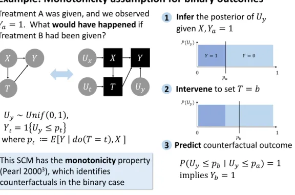
For instance, suppose that 𝑌 corresponds to a favorable binary outcome, such as 5-year survival, and 𝑇 corresponds to a treatment. Then several quantities of interest in causal effect estimation, including (but not limited to) the ATE and the CATE, are defined by the interventional distribution, which is forward-looking, telling us what might be expected to occur if we applied an intervention. However, we can also define the counterfactual distribution which is retrospective, telling us what might have happened had we acted differently. For instance, we might ask: Having given the drug and observed that 𝑌 = 1 (survival), what would have happened if we had instead withheld the drug? This is formalized in an SCM as follows:
Definition 3 (Counterfactual Distribution). Given an SCM ℳ and an observed assignment X = x over any set of observed variables, the counterfactual distribution 𝑃𝑋ℳ|X=x;𝐼 corresponds to the distribution entailed by the SCM ℳ𝐼 using the posterior distribution 𝑃 (U|X = x).
Explicitly, given an SCM ℳ, the counterfactual distribution can be estimated by first inferring the posterior over latent variables, e.g., 𝑃 (U|X = x, 𝑇 = 1, 𝑌 = 1) in our running example, and then passing that distribution through the structural
mechanisms in a modified ℳ𝐼 (e.g., 𝐼 = 𝑑𝑜(𝑇 = 0)) to obtain a counterfactual distribution over any variable5. In this way, we make precise the meaning of several terms we will use in this thesis. When we say counterfactual inference, we are referring to this process of obtaining a counterfactual distribution. Similarly, we sometimes use the term counterfactual posterior to refer to the counterfactual distribution, to reflect the fact that it is simply posterior inference in a particular type of causal model.
2.3.3
Non-Identifiability of Binary SCMs
So, given an SCM ℳ, we can compute an answer to our counterfactual question: Having given the drug and observed that 𝑌 = 1 (survival), what would have happened if we had instead withheld the drug? In the binary case, this corresponds to the Probability of Necessity (PN) (Pearl, 2009; Dawid et al., 2015), because it represents the probability that the exposure 𝑇 = 1 was necessary for the outcome.
Intuitively, this is impossible to answer with certainty, even though we may ask ourselves these types of questions frequently in the real world. For instance, in medical malpractice, establishing fault requires just such a counterfactual claim, showing that an injury would not have occurred “but for” the breach in the standard of care (Bal, 2009; Encyclopedia, 2008).
Mathematics matches our intuition in this case: The answer to the question is not identifiable without further assumptions, a general property of counterfactual infer-ence. That is, there are multiple SCMs which are all consistent with the interventional distribution, but which produce different counterfactual estimates of quantities like the Probability of Necessity (Pearl, 2009).
2.3.4
Monotonicity Assumption for Identification of Binary
SCMs
Nonetheless, there are plausible (though untestable) assumptions we can make that identify counterfactual distributions. Consider our intuition in the following case: